Renaming a column in excel

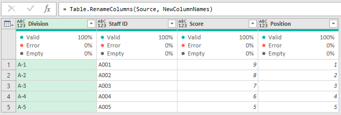
Rename a column (Power Query)

You can rename a column header to make it more clear. You can only rename one column at a time.

Note To prevent a column name conflict from other commands that create column, Power Query disambiguates by creating a unique name. In these cases, you often want to rename them. But table column names must be unique for all columns. Renaming a column to a column name that already exists creates an error.

To open a query, locate one previously loaded from the Power Query Editor, select a cell in the data, and then select Query > Edit. For more information see Create, load, or edit a query in Excel.

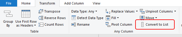
Select a column, and then select Transform > Rename. You can also double-click the column header.

Enter the new name.

Renaming a column header in Power Query doesn’t rename the original data source column header. Avoid renaming the column header in the data source because it can cause query errors. But it’s possible someone else could change the column header in an imported external data source. If this happens, you can receive the error:

“The column ‘ ‘ of the table wasn’t found.”

To correct the query error, select Go To Error in the yellow message box, and correct the formula in the formula bar. But proceed carefully. Whenever you change a previous step under Applied Steps in the Query Settings pane, subsequent steps might also be affected. To confirm your fix, refresh the data by selecting Home > Refresh Preview > Refresh Preview.

Источник

How to change the name of the column headers in Excel

In Microsoft Excel, the column headers are named A, B, C, and so on by default. Some users want to change the names of the column headers to something more meaningful. Unfortunately, Excel does not allow the header names to be changed.

The same applies to row names in Excel. You cannot change the row names, or numbering, but you can add your desired row names in column A for the corresponding rows.

Instead, if you want to have meaningful column header names, you can do the following.

1. Click in the first row of the worksheet and insert a new row above that first row.

• How to add or remove a cell, column, or row in Excel.

1. In the inserted row, enter the preferred name for each column.
2. To make the row of column names more noticeable, you could increase the text size, make the text bold, or add background color to the cells in that row.

After inserting the new row and adding column header names, if you want to hide the default column header names, follow the steps below to hide column and row headers.

1. In Microsoft Excel, click the File tab or the Office button in the upper-left corner.
2. In the left navigation pane, click Options.
3. In the Excel Options window, click the Advanced option in the left navigation pane.
4. Scroll down to the Display options for this worksheet section. Uncheck the box for Show row and column headers.

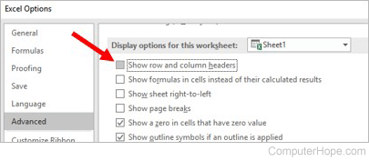
The column and row headers are now hidden. To display them again, re-check the box in step 4 above.

Источник

How to Name Columns in Excel for Office 365

posted on October 13, 2022

While many people will use a header row in their spreadsheets to identify the information that is contained within a column, that might not be useful for what you need to do.

Another option that you have involves learning how to name a column in Excel.

This gives you some additional flexibility with cell references and formulas, which may be more optimal for the way that you use Excel.

Our tutorial below will show you how to name columns in Excel so that you can start taking advantage of the additional features this enables.

How to Title Columns in Excel

1. Open your spreadsheet.
2. Click the column letter to rename.
3. Click in the Name field next to the formula bar.
4. Delete the current name.
5. Enter the new name, then press Enter.

Our article continues below with additional information on naming columns in Excel for office 365, including pictures of these steps.

When you need to reference a specific cell in Microsoft Excel it is common for you to use row numbers and column letters. These are shown at the left side and top of the spreadsheet, respectively, and provide an easy way to locate cells for formulas.

But you may be looking for a way to create custom column names in Excel if you don’t want to use the default column headings.

This can be useful when you are working with a lot of similar data and are running into problems with properly identifying columns. It can also be a useful way to may writing formulas easier because you can just enter your custom name into the formula rather than going back to see which column contains which data.

Fortunately, it is possible for you to give a column a name in Excel if you would like to be able to reference the column by that name rather than the standard column letters.

How to Rename a Column in Excel (Guide with Pictures)

the steps in this article were performed in the desktop version of the Microsoft Excel for Office 365 application. However, these steps will also work in most other versions of Excel.

These steps will show you how to label columns in Excel.

Step 1: Open the Excel file containing the column you wish to rename.

Open your spreadsheet.

Step 2: Click the column letter above the spreadsheet.

Choose the letter of the column to name.

Step 3: Click inside the Name field that is above the row numbers and to the left of the formula bar.

Select the Name field.

It is at the upper left corner of the Excel worksheet, above the row numbers and to the left of the column letters.

Step 4: Delete the current column name.

Remove the existing column name.

Step 5: Type the new name, then press Enter on your keyboard.

Input the new column name and press Enter.

Now that you know how to name a column in Excel you can take advantage of this when you are working on spreadsheets that need column names.

The next section discusses editing a column header in Excel.

How to Change a Column Header in the Name Box Dropdown List in Microsoft Excel

The steps above walk you through the process of how you create names for single columns in an Excel spreadsheet. Once you have elected to give a new, custom name rather than the default Excel names for some of your columns, then those custom names are going to appear in a dropdown list within the Name field.

You can quickly select a column and choose to rename one of these column headers by simply clicking inside that Name field and choosing the column name. That will select that column. You can then click inside the Name field again, delete the current name, enter a new name, then press Enter.

Our guide continues below with more information, such as what to do if you are seeing an error when trying to name columns in Excel.

More Information on How to Name Columns in Excel

If the row numbers and columns aren’t visible in Microsoft Excel then they have probably been hidden. You can display them by selecting the View tab at the top of the window, then checking the box next to Headings in the Show group of the ribbon.

If you are having trouble giving your column a name, then it may be because you are attempting to include a space. In my example above I am giving my column the name “LastName” but I would get an error if I tried to give it a name of “Last Name.”

Once a column is renamed you can do stuff like =SUM(LastName) to quickly add all of the values in that column.

One helpful thing that you can do when you have renamed columns in Excel is to quickly select an entire column by its name. if you click the arrow in the Name field you will see a dropdown list with all of your custom column names. If you select one of those names it will automatically highlight that entire column.

These column names are a little different than creating titles in the first row of each column. Traditionally that is used as a simple way to identify what type of data is in a column. It also makes it very easy to use the “Print Titles” button on the Page Layout tab so that you can repeat the top row of your spreadsheet on every page.

it is possible for you to use the first row as a title row in Microsoft Excel while still creating custom column names using the steps outlined in the tutorial above.

One additional similar action you can take is to create an Excel named range that consists of a few cells. You can use your mouse to select the cells to include in that range, then click inside the Name field, delete the current name, enter the new one, then press Enter on the keyboard. When you start creating more and more named ranges in your spreadsheet you can really make selections quickly by clicking the Name Manager to cycle through all of your defined names group values.

Frequently Asked Questions About How to Name a Column in Excel

Are headers and column names the same thing in Excel?

No, these are two different things.

A header in Excel is the first row of the spreadsheet, where you can enter a word or phrase that describes the information that will appear in cells in that column.

A name is something that you apply with the special “Name” field to the left of the column letters.

An Excel header and name can have the same values, but they serve different purposes.

Often row headers will be sufficient for an Excel sheet.

Where is the Excel formula bar?

you can find the formula bar in your Excel spreadsheet above the column letters.

It is possible to hide the formula bar, however, you can also go to the View tab, then make sure that the Formula Bar option in the Show group is checked.

How do I delete a column in Microsoft Excel?

If you have a column in your Excel document that you don’t need anymore, then you are able to remove it.

You can do this by right-clicking on the column letter, then choosing the Delete option.

You can also use this option to delete multiple columns.

Simply hold down the Ctrl key on your keyboard, then click each column letter that you want to remove.

Once all of the columns are selected you can right-click on one of them and choose the Delete option.

Matthew Burleigh has been a freelance writer since the early 2000s. You can find his writing all over the Web, where his content has collectively been read millions of times.

Matthew received his Master’s degree in Computer Science, then spent over a decade as an IT consultant for small businesses before focusing on writing and website creation.

Источник

Renaming Columns A, B, C, D, E, etc. in Excel?

Lee H.

How can a user rename Column «A» to say «Last Name,» rename Column «B» to say
«First Name,» Column «C» to say «Address 1,» etc?

This would allow the data to start on row #1 for automatic renumbering when
new rows are added, rather than having to put the column names on row 1,
causing the data to start on row 2.

Advertisements

Dave Peterson

You can show letters or numbers as the column headers—or hide them. But you
can’t rename them.

ShaneDevenshire

You can «sort of» do this 2007:

1. Select the range and choose Home, Format as Table and pick a style
2. As you scroll down the screen the column letters will be replaced with
the titles in the table when you reach the limit of viewing the titles.

Crenz

Thank you very much Shane! So simple, yet so elegant!

I had seen this done in a spreadsheet and wondered how it was done. Searched the net extensively with several different keyword patterns, didn’t find what I was looking for. until I stumbled upon your response. This is the only response I have seen so far and it is perfect.

Thanks once again.

Cren

You can «sort of» do this 2007:

1. Select the range and choose Home, Format as Table and pick a style
2. As you scroll down the screen the column letters will be replaced with
the titles in the table when you reach the limit of viewing the titles.

—
Thanks,
Shane Devenshire

«Lee H.» wrote:

> How can a user rename Column «A» to say «Last Name,» rename Column «B» to say
> «First Name,» Column «C» to say «Address 1,» etc?
>
> This would allow the data to start on row #1 for automatic renumbering when
> new rows are added, rather than having to put the column names on row 1,
> causing the data to start on row 2.

Источник

Renaming columns in excel

We have many different tables to be appended. It should be a simple task with Power Query. You may refer to my blogpost here for the basic of appending tables with Power Query. Nevertheless, life could be challenging in workplace. What if the tables do not have consistent column names? We need to convert all the column names into common names before appending tables. Are we going to read and rename all column names table by table, manually? Of course not! And this is exactly the reason for this post! 😉

Inspirations and the Thinking Process:

Before jumping to the solution, I would like to share with you the inspirations and the thinking process behind the scene.

Indeed, I came across this topic from a video by Leila Gharani. In the video she demonstrated how to solve the problem in a very elegant (and advanced) way with M code using the function List.Accumulate. You can see the formula she used in the following screenshot.

To be perfectly honest, it is out of my comprehension. I watched the video a couple of times. I kind of understand it while she explained along but I knew I could not write that formula by myself. It’s still a long way for me to do so. 😅

I love Power Query because it empowers non-programmer like me to do super powerful stuffs.

So, I have been thinking for quite a long time: Can I solve the problem

• by using mainly elements on the user interface of Power Query Editor…
• without using advanced M code…
• well, probably with some simple formula (basic M code)?

Then I started doing experiments (or put it in other words, trial and error). The first thing I did was to examine the code auto-generated when I renamed columns manually.

Well… it seems to be a simple line of code. The function involved is Table.RenameColumns. Then I further drilled into the description of the function which requires two parameters:

1. table as table
2. renames as list

umm… what does that mean?

The first parameter is simple. It’s a table. Usually it refers to previous step (but not necessary).

But what about the second parameter? A list of two values, provided in a list?

Let’s look at the auto-generated code again:

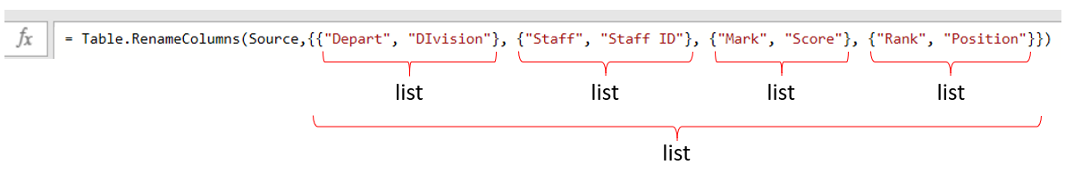
A list is enclosed by a pair of < >. The code above contains a list of list. I realized that as long as I can create a dynamic list of list (with two values) and then feed it into the second parameter of the function, I should be able to rename columns in a dynamic way, with the help of a conversion table.

A conversion table is a predefined list of (inconsistent) headers anticipated, and the corresponding list of common (consistent) headers.

I know how to convert a column into a list. That is super easy by using Convert to List on the Transform tab of Power Query Editor.

Tip: This can also be achieved by right-clicking a column header, followed by Drill Down.

However, there is no easy way to convert two columns into a list of list.

I tried many different ways without success. I was a bit frustrated. I wondered if that’s possible, Leila should have done it and demonstrated it in another video. So I gave it up. 😁

Then today I came across a video by Oz from Excel On Fire. Indeed It has nothing related to the problem we discussed above. In the video Oz showed how to split text from a column using the function Text.Split. At 2:08 in the video, after he added a custom column using Text.Split, the result showed on the screen was the light-bulb moment to me!

Did you see that? The result returns a List. Bravo! This is exactly what I need. I can’t stop myself from testing it in Excel. It works!

Solution

It’s time to show my solution. If you are still with me, I expect you have some knowledge in Power Query. Therefore the following will not be a step-by-step tutorial but the key transformation steps required.

You may download a sample file to follow along.

First thing first. Load the tables to Power Query.

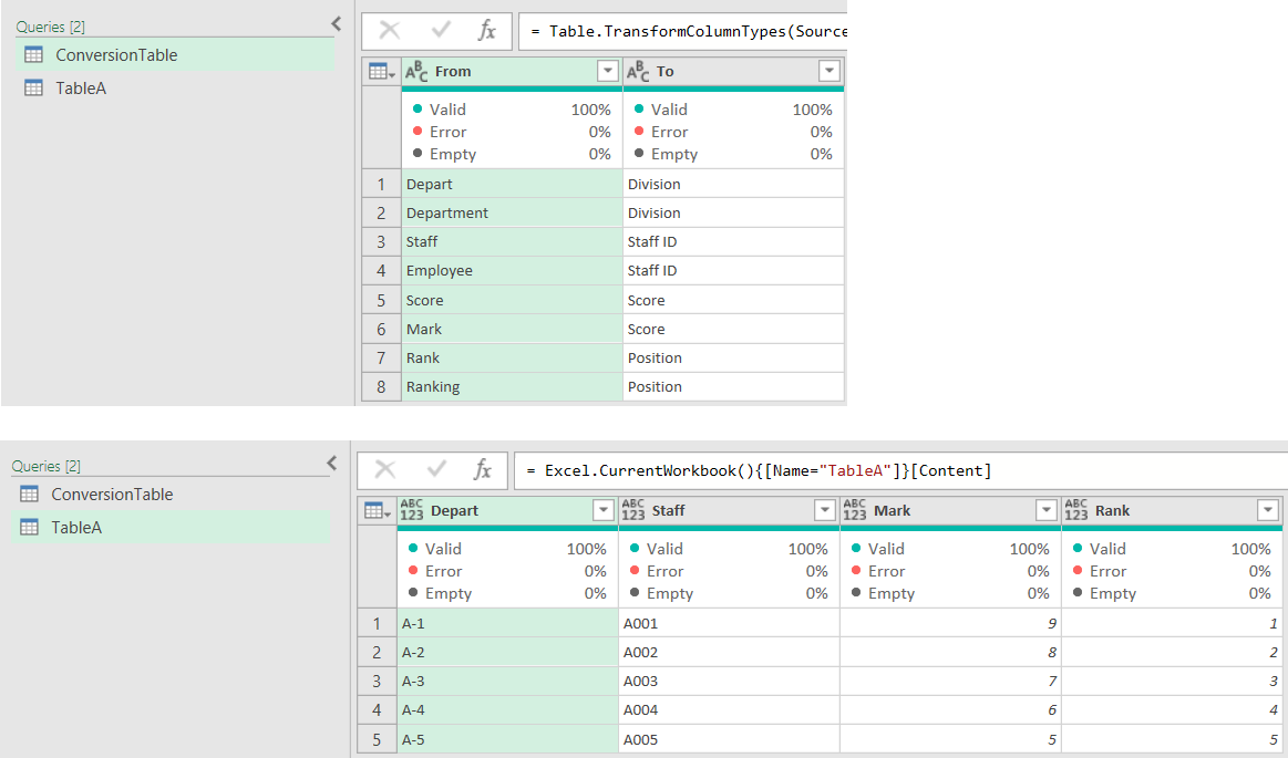
Now we have TableA, i.e. the table with headers needed to be changed, based on the content in the Conversion Table.

Get the column names of TableA

To get the column names of TableA, I added a custom step by using the following formula:

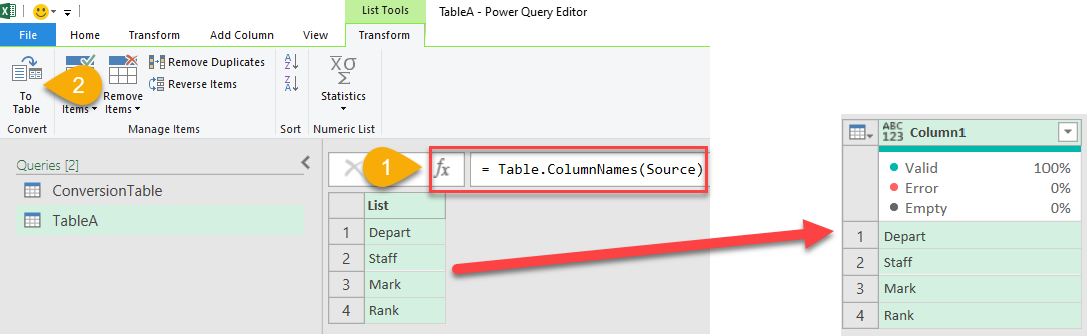
The result was a List. I turned the resulting list to a Table.

Get the “New” Column Name by Merging Query

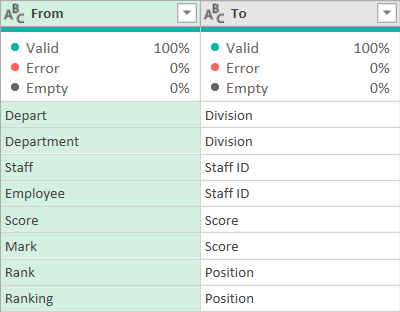
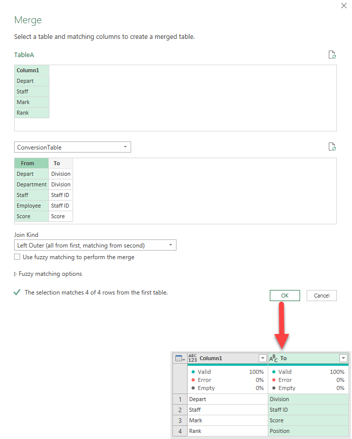
I performed a Left-Outer Merge with the Conversion Table, as shown below:

Convert the two columns into a list of list (with two values)

Here’s the tricky part that I got stuck for long, until I watched Oz’s video.

In order to create the list of list, I merged the two columns first.

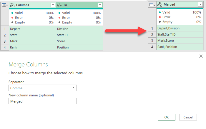Note: I chose “Comma” as the separator

Then, I split it by adding a Custom Column using the function Text.Split.

Here’s the formula used for this step:

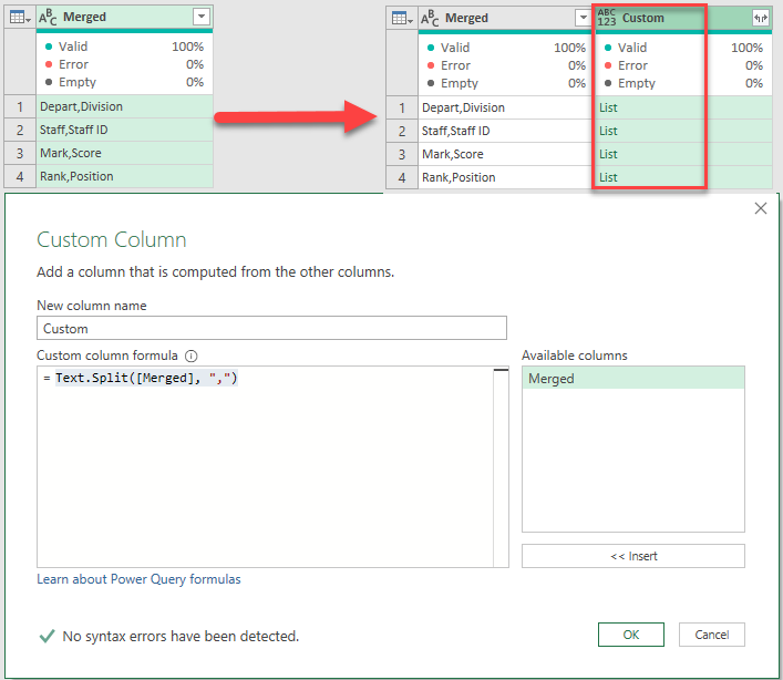
Now I’ve got a list of two values. The next step is get create a list of list.

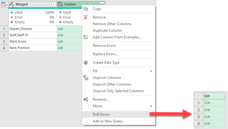Right-Click the column header [Custom] ==> Drill Down

YESSS! I had just created the list of list that I have been looking for.

Then I renamed the last step from “Custom” to “NewColumnNames” (just to make the next step more readable).

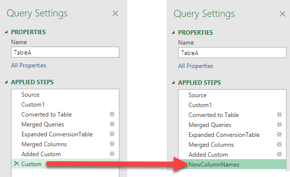
Rename Column Names dynamically

The final step has become easy. Do you still remember the auto-generated code for renaming columns?

What we need to do here is to add a custom step with the same formula, but substituting the second hard-coded parameter by NewColumnNames.

Can you believe it? It is done!

Testing the result

As always, we have to test the result to see if it is working as expected. Let’s change the conversion table and see what happens:

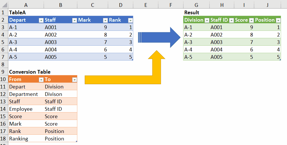The column names updated per changes on Conversion Table!

Now let’s change the headers and see:

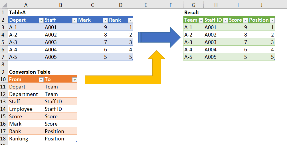The result gives consistent column names!

You may also download a sample file with the queries:

Application – Append tables with different column names

With this technique, we can combine workbooks with inconsistent column headers with ease. This would be better illustrated with a video, which is under production. Stay tuned! 😉

Источник

While many people will use a header row in their spreadsheets to identify the information that is contained within a column, that might not be useful for what you need to do.

Another option that you have involves learning how to name a column in Excel.

This gives you some additional flexibility with cell references and formulas, which may be more optimal for the way that you use Excel.

Our tutorial below will show you how to name columns in Excel so that you can start taking advantage of the additional features this enables.

1. Open your spreadsheet.
2. Click the column letter to rename.
3. Click in the Name field next to the formula bar.
4. Delete the current name.
5. Enter the new name, then press Enter.

Our article continues below with additional information on naming columns in Excel for office 365, including pictures of these steps.

When you need to reference a specific cell in Microsoft Excel it is common for you to use row numbers and column letters. These are shown at the left side and top of the spreadsheet, respectively, and provide an easy way to locate cells for formulas.

But you may be looking for a way to create custom column names in Excel if you don’t want to use the default column headings.

This can be useful when you are working with a lot of similar data and are running into problems with properly identifying columns. It can also be a useful way to may writing formulas easier because you can just enter your custom name into the formula rather than going back to see which column contains which data.

Fortunately, it is possible for you to give a column a name in Excel if you would like to be able to reference the column by that name rather than the standard column letters.

How to Rename a Column in Excel (Guide with Pictures)

the steps in this article were performed in the desktop version of the Microsoft Excel for Office 365 application. However, these steps will also work in most other versions of Excel.

Now that you know how to name a column in Excel you can take advantage of this when you are working on spreadsheets that need column names.

The next section discusses editing a column header in Excel.

How to Change a Column Header in the Name Box Dropdown List in Microsoft Excel

The steps above walk you through the process of how you create names for single columns in an Excel spreadsheet. Once you have elected to give a new, custom name rather than the default Excel names for some of your columns, then those custom names are going to appear in a dropdown list within the Name field.

You can quickly select a column and choose to rename one of these column headers by simply clicking inside that Name field and choosing the column name. That will select that column. You can then click inside the Name field again, delete the current name, enter a new name, then press Enter.

Our guide continues below with more information, such as what to do if you are seeing an error when trying to name columns in Excel.

More Information on How to Name Columns in Excel

If the row numbers and columns aren’t visible in Microsoft Excel then they have probably been hidden. You can display them by selecting the View tab at the top of the window, then checking the box next to Headings in the Show group of the ribbon.

If you are having trouble giving your column a name, then it may be because you are attempting to include a space. In my example above I am giving my column the name “LastName” but I would get an error if I tried to give it a name of “Last Name.”

Once a column is renamed you can do stuff like =SUM(LastName) to quickly add all of the values in that column.

One helpful thing that you can do when you have renamed columns in Excel is to quickly select an entire column by its name. if you click the arrow in the Name field you will see a dropdown list with all of your custom column names. If you select one of those names it will automatically highlight that entire column.

These column names are a little different than creating titles in the first row of each column. Traditionally that is used as a simple way to identify what type of data is in a column. It also makes it very easy to use the “Print Titles” button on the Page Layout tab so that you can repeat the top row of your spreadsheet on every page.

it is possible for you to use the first row as a title row in Microsoft Excel while still creating custom column names using the steps outlined in the tutorial above.

One additional similar action you can take is to create an Excel named range that consists of a few cells. You can use your mouse to select the cells to include in that range, then click inside the Name field, delete the current name, enter the new one, then press Enter on the keyboard. When you start creating more and more named ranges in your spreadsheet you can really make selections quickly by clicking the Name Manager to cycle through all of your defined names group values.

Frequently Asked Questions About How to Name a Column in Excel