
Excel is an awesome tool. The more I learn about it the more I fall in love with it.
The team that has built Excel has put in a lot of thinking behind it and they continuously work on improving the user experience.
But there are still somethings that I find irritating and often need to change the default settings.
And one such thing is dotted lines in the worksheet in Excel.
In this tutorial, I will show you the possible reasons why these dotted lines appear and how to remove these dotted lines.
So let’s get started!
Possible Reasons for Dotted Lines in Excel
There can be various reasons for the dotted lines to appear in Excel:
- Due to Page breaks where Excel visually show page breaks as dotted lines
- Borders that have been set to show as dotted lines
- Gridlines that appear in the whole worksheet. These are not really dotted lines (rather faint solid lines that looks like dotted borders around the cells)
Your worksheet can have any one or more of these settings and you can easily remove these lines and disable it.
How to Remove Dotted Lines in Excel
Let’s dive in and see how to remove these dotted lines in Excel in each scenario.
Removing the Page Break Dotted Lines
This is one of the most irritating things for me in Excel. Sometimes, I see these page-breaks dotted lines (as shown below) that just refuse to go away.

Now, I understand the utility and purpose of keeping these. It divides your worksheet into sections and you would know what part will be printed on one page and what will spill over.
A super easy (but not ideal) fix of this is to close the workbook and open again. Reopening a workbook will remove the page break dotted lines.
Here is a better way to remove these dotted lines:
- Click on the File tab

- Click on Options

- In the Excel Options dialog box that opens, click on the Advanced option in the left pane

- Scroll down to the section – “Display options for this worksheet”

- Uncheck the option – “Show page breaks”


The above steps would stop showing the page break dotted line for the workbook.
Note that the above steps would stop showing the dotted lines only for the workbook in which you have unchecked this option. For other workbooks, you will have to repeat the same process if you want to get rid of the dotted lines.
In case you have set the print area in the worksheet, the dotted lines will not be shown. Instead, you will see solid lined outlining the print area.
Removing Dotted Lines Border
In some cases (not as common as page break though), people may use dotted lines as the border.
Something as shown below:

To remove these dotted lines, you can either remove the border completely or change the dotted line border to the regular solid line border.
Below are the steps to remove these dotted borders:
- Select the cells from which you want to remove the dotted border
- Click the Home tab

- In the Font group, click on the ‘Border’ drop-down

- In the border options that appear, click on ‘No Border’


The above steps would remove any borders in the selected cells.
In case you want to replace the dotted border with some other type of border, you can do that as well.
Removing Gridlines
While the gridlines are not dotted lines (these are solid lines), some people still think that these look like dotted lines (as these are quite faint).
These gridlines are applied to the entire worksheet and you can easily make them disappear.
Below are the steps to remove these:
- Click on the View tab

- In the Show group, uncheck the Gridlines option


That’s it! The above steps would remove all the gridlines from the worksheet. In case you want the Gridlines back, simply go back and check the same option.
So these are three ways you can remove the dotted lines in Excel.
I hope you found this tutorial useful!
Some Other Excel tutorials you may also like:
- How to Remove Line Breaks in Excel
- How to Remove Table Formatting in Excel
- Use Format Painter in Excel to Quickly Copy Formatting
- How to Split a Cell Diagonally in Excel (Insert Diagonal Line)
- How to Insert/Draw a Line in Excel (Straight Line, Arrows, Connectors)
Specific line and bar types are available in 2-D stacked bar and column charts, line charts, pie of pie and bar of pie charts, area charts, and stock charts.
Predefined line and bar types that you can add to a chart
Depending on the chart type that you use, you can add one of the following lines or bars:
-
Series lines These lines connect the data series in 2-D stacked bar and column charts to emphasize the difference in measurement between each data series. Pie of pie and bar of pie charts display series lines by default to connect the main pie chart with the secondary pie or bar chart.

-
Drop lines Available in 2-D and 3-D area and line charts, these lines extend from data points to the horizontal (category) axis to help clarify where one data marker ends and the next data marker starts.
-
High-low lines Available in 2-D line charts and displayed by default in stock charts, high-low lines extend from the highest value to the lowest value in each category.
-
Up-down bars Useful in line charts with multiple data series, up-down bars indicate the difference between data points in the first data series and the last data series. By default, these bars are also added to stock charts, such as Open-High-Low-Close and Volume-Open-High-Low-Close.
Add predefined lines or bars to a chart
-
Click the 2-D stacked bar, column, line, pie of pie, bar of pie, area, or stock chart to which you want to add lines or bars.
This displays the Chart Tools, adding the Design, Layout, and Format tabs.
-
On the Layout tab, in the Analysis group, do one of the following:
-
Click Lines, and then click the line type that you want.
Note: Different line types are available for different chart types.
-
Click Up/Down Bars, and then click Up/Down Bars.
-
Tip: You can change the format of the series lines, drop lines, high-low lines, or up-down bars that you display in a chart by right-clicking the line or bar, and then clicking Format <line or bar type> .
Remove predefined lines or bars from a chart
-
Click the 2-D stacked bar, column, line, pie of pie, bar of pie, area, or stock chart that displays predefined lines or bars.
This displays the Chart Tools, adding the Design, Layout, and Format tabs.
-
On the Layout tab, in the Analysis group, click Lines or Up/Down Bars, and then click None to remove lines or bars from a chart.
Tip: You can also remove lines or bars immediately after you add them to the chart by clicking Undo on the Quick Access Toolbar or by pressing CTRL+Z.
You can add other lines to any data series in an area, bar, column, line, stock, xy (scatter), or bubble chart that is 2-D and not stacked.
Add other lines
-
This step applies to Word for Mac only: On the View menu, click Print Layout.
-
In the chart, select the data series that you want to add a line to, and then click the Chart Design tab.
For example, in a line chart, click one of the lines in the chart, and all the data marker of that data series become selected.
-
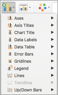
Click Add Chart Element, and then click Gridlines.
-
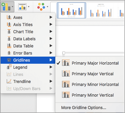
Choose the line option that you want or click More Gridline Options.
Depending on the chart type, some options may not be available.
Remove other lines
-
This step applies to Word for Mac only: On the View menu, click Print Layout.
-
Click the chart with the lines, and then click the Chart Design tab.
-
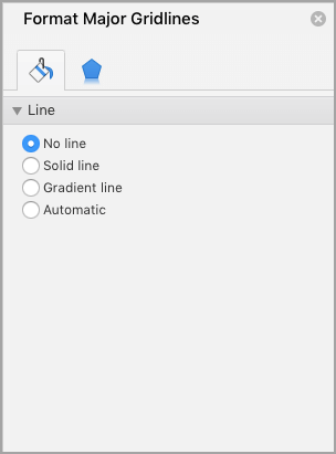
Click Add Chart Element, click Gridlines, and then click More Gridline Options.
-
Select No line.
You can also click the line and press DELETE .
Содержание
- Add or remove series lines, drop lines, high-low lines, or up-down bars in a chart
- Predefined line and bar types that you can add to a chart
- Add predefined lines or bars to a chart
- Remove predefined lines or bars from a chart
- Add other lines
- Remove other lines
- How to delete blank rows in Excel quickly and safely
- How NOT to remove blank lines in Excel
- How to remove blank rows in Excel with VBA
- Macro 1. Delete blank lines in a selected range
- Macro 2. Delete all blank rows in Excel
- Macro 3. Delete row if cell is blank
- How to remove blank lines in Excel with VBA
- Add a macro to your workbook
- Run a macro from our sample workbook
- Formula to delete blank rows in Excel
- How to remove empty lines in Excel with Power Query
- How to delete rows if cell in a certain column is blank
- How to remove extra lines below data
- Fastest way to remove empty rows in Excel
Add or remove series lines, drop lines, high-low lines, or up-down bars in a chart
You can add predefined lines or bars to charts in several apps for Office. By adding lines, including series lines, drop lines, high-low lines, and up-down bars, to specific chart can help you analyze the data that is displayed. If you no longer want to display the lines or bars, you can remove them.
New to formatting charts in Excel? Click here for a free 5 minute video training on how to format your charts.
Specific line and bar types are available in 2-D stacked bar and column charts, line charts, pie of pie and bar of pie charts, area charts, and stock charts.
Predefined line and bar types that you can add to a chart
Depending on the chart type that you use, you can add one of the following lines or bars:
Series lines These lines connect the data series in 2-D stacked bar and column charts to emphasize the difference in measurement between each data series. Pie of pie and bar of pie charts display series lines by default to connect the main pie chart with the secondary pie or bar chart. 
Drop lines Available in 2-D and 3-D area and line charts, these lines extend from data points to the horizontal (category) axis to help clarify where one data marker ends and the next data marker starts. 
High-low lines Available in 2-D line charts and displayed by default in stock charts, high-low lines extend from the highest value to the lowest value in each category. 
Up-down bars Useful in line charts with multiple data series, up-down bars indicate the difference between data points in the first data series and the last data series. By default, these bars are also added to stock charts, such as Open-High-Low-Close and Volume-Open-High-Low-Close. 
Add predefined lines or bars to a chart
Click the 2-D stacked bar, column, line, pie of pie, bar of pie, area, or stock chart to which you want to add lines or bars.
This displays the Chart Tools, adding the Design, Layout, and Format tabs.
On the Layout tab, in the Analysis group, do one of the following:
Click Lines, and then click the line type that you want.
Note: Different line types are available for different chart types.
Click Up/Down Bars, and then click Up/Down Bars. 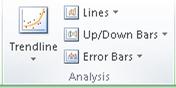
Tip: You can change the format of the series lines, drop lines, high-low lines, or up-down bars that you display in a chart by right-clicking the line or bar, and then clicking Format .
Remove predefined lines or bars from a chart
Click the 2-D stacked bar, column, line, pie of pie, bar of pie, area, or stock chart that displays predefined lines or bars.
This displays the Chart Tools, adding the Design, Layout, and Format tabs.
On the Layout tab, in the Analysis group, click Lines or Up/Down Bars, and then click None to remove lines or bars from a chart.
Tip: You can also remove lines or bars immediately after you add them to the chart by clicking Undo on the Quick Access Toolbar or by pressing CTRL+Z.
You can add other lines to any data series in an area, bar, column, line, stock, xy (scatter), or bubble chart that is 2-D and not stacked.
Add other lines
This step applies to Word for Mac only: On the View menu, click Print Layout.
In the chart, select the data series that you want to add a line to, and then click the Chart Design tab.
For example, in a line chart, click one of the lines in the chart, and all the data marker of that data series become selected.
Click Add Chart Element, and then click Gridlines.
Choose the line option that you want or click More Gridline Options.
Depending on the chart type, some options may not be available.
Remove other lines
This step applies to Word for Mac only: On the View menu, click Print Layout.
Click the chart with the lines, and then click the Chart Design tab.
Click Add Chart Element, click Gridlines, and then click More Gridline Options.
You can also click the line and press DELETE .
Источник
How to delete blank rows in Excel quickly and safely
 by Svetlana Cheusheva, updated on March 16, 2023
This tutorial will teach you a few simple tricks to delete multiple empty rows in Excel safely without losing a single bit of information.
Blank rows in Excel is a problem we all face once in a while, especially when combining data from different sources or importing information from somewhere else. Empty lines can cause a lot of havoc to your worksheets on different levels and deleting them manually can be a time-consuming and error-prone process. In this article, you will learn a few simple and reliable methods to remove blanks in your worksheets.
How NOT to remove blank lines in Excel
There are a few different ways to delete empty lines in Excel, but surprisingly many online resources stick with the most dangerous one, namely Find & Select > Go To Special > Blanks.
What’s wrong about this technique? It selects all blanks in a range, and consequently you will end up deleting all rows that contain as much as a single blank cell.
The below image shows the original table on the left and the resulting table on the right. And in the resulting table, all incomplete rows ae gone, even row 10 where only the date in column D was missing:
![]()
The bottom line: if you don’t want to mess up your data, never delete empty rows by selecting blank cells. Instead, use one of the more considered approaches discussed below.
How to remove blank rows in Excel with VBA
Excel VBA can fix a lot of things, including multiple empty rows. The best thing about this approach is that it does not require any programming skills. Simply, grab one of the below codes and run it in your Excel (the instructions are here).
Macro 1. Delete blank lines in a selected range
This VBA code silently deletes all blank rows in a selected range, without showing any message or dialog box to the user.
Unlike the previous technique, the macro deletes a line if the entire row is empty. It relies on the worksheet function CountA to get the number of non-empty cells in each line, and then deletes rows with the zero count.
To give the user an opportunity to select the target range after running the macro, use this code:
Upon running, the macro shows the following input box, you select the target range, and click OK:
![]()
In a moment, all empty lines in the selected range will be eliminated and the remaining ones will shift up:
![]()
Macro 2. Delete all blank rows in Excel
To remove all blank rows on the active sheet, determine the last row of the used range (i.e. the row containing the last cell with data), and then go upwards deleting the lines for which CountA returns zero:
Macro 3. Delete row if cell is blank
With this macro, you can delete an entire row if a cell in the specified column is blank.
The following code checks column A for blanks. To delete rows based on another column, replace «A» with an appropriate letter.
As a matter of fact, the macro uses the Go To Special > Blanks feature, and you can achieve the same result by performing these steps manually.
Note. The macro deletes blank rows in the entire sheet, so please be very careful when using it. As a precaution, it may be wise to back up the worksheet before running this macro.
How to remove blank lines in Excel with VBA
To delete empty rows in Excel using a macro, you can either insert the VBA code into your own workbook or run a macro from our sample workbook.
Add a macro to your workbook
To insert a macro in your workbook, perform these steps:
- Open the worksheet where you want to delete blank rows.
- Press Alt + F11 to open the Visual Basic Editor.
- On the left pane, right-click ThisWorkbook, and then click Insert >Module.
- Paste the code in the Code window.
- Press F5 to run the macro.
For the detailed step-by-step instructions, please see How to insert and use VBA in Excel.
Run a macro from our sample workbook
Download our sample workbook with Macros to Delete Blank Rows and run one of the following macros from there:
DeleteBlankRows — removes empty rows in the currently selected range.
RemoveBlankLines — deletes blank rows and shifts up in a range that you select after running the macro.
DeleteAllEmptyRowsВ — deletes all empty lines on the active sheet.
DeleteRowIfCellBlank — deletes a row if a cell in a specific column is blank.
To run the macro in your Excel, do the following:
- Open the downloaded workbook and enable the macros if prompted.
- Open your own workbook and navigate to the worksheet of interest.
- In your worksheet, press Alt + F8, select the macro, and click Run.
Formula to delete blank rows in Excel
In case you’d like to see what you are deleting, use the following formula to identify empty lines:
=IF(COUNTA(A2:D2)=0, «Blank», «Not blank»)
Where A2 is the first and D2 is the last used cell of the first data row.
Enter this formula in E2 or any other blank column in row 2, and drag the fill handle to copy the formula down.
As the result, you will have «Blank» in empty rows and «Not blank» in the rows that contain at least one cell with data:
![]()
The formula’s logic is obvious: you count non-empty cells with the COUNTA function and use the IF statement to return «Blank» for zero count, «Not Blank» otherwise.
In fact, you can do nicely without IF:
In this case, the formula will return TRUE for blank lines and FALSE for non-blank lines.
With the formula in place, carry out these steps to delete empty lines:
- Select any cell in the header row and click Sort & Filter >Filter on the Home tab, in the Formats This will add the filtering drop-down arrows to all header cells.
- Click the arrow in the formula column header, uncheck (Select All), select Blank and click OK:
![]()
![]()
That’s it! As the result, we have a clean table with no blank lines, but all the information preserved:
![]()
Tip. Instead of deleting empty lines, you can copy non-empty rows to somewhere else. To have it done, filter «Not blank» rows, select them and press Ctrl + C to copy. Then switch to another sheet, select the upper-left cell of the destination range and press Ctrl + V to paste.
How to remove empty lines in Excel with Power Query
In Excel 2016 and Excel 2019, there is one more way to delete empty rows — by using the Power Query feature. In Excel 2010 and Excel 2013, it can be downloaded as an add-in.
Important note! This method works with the following caveat: Power Query converts the source data into an Excel table and changes the formatting such as fill color, borders and some number formats. If the formatting of your original data is important to you, then you’d better choose some other way to remove blank rows in Excel.
- Select the range where you want to delete empty lines.
- Go to the Data tab >Get & Transform group and click From Table/Range. This will load your table to the Power Query Editor.

On the Home tab of the Power Query Editor, click Remove Rows >Remove Blank Rows.
![]()
Click the Close & Load This will load the resulting table to a new worksheet and close the Query Editor.
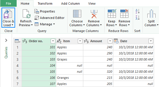
In the result of these manipulations, I got the following table without empty lines, but with a couple of nasty changes — the currency format is lost and the dates are displayed in the default format instead of the custom one:

How to delete rows if cell in a certain column is blank
In the beginning of this tutorial, we warned you against removing empty lines by selecting blanks. However, this method comes in handy if you want to delete rows based on blanks in a specific column.
As an example, let’s remove all the rows where a cell in column A is empty:
- Select the key column, column A in our case.
- On the Home tab, click Find & Select >Go To Special. Or press F5 and click the Special… button.

In the Go To Special dialog, select Blanks and click OK. This will select blank cells in the used range in column A.
![]()
![]()
Done! The rows that do not have a value in column A are no longer there:
![]()
The same result can be achieved by filtering blanks in the key column.
Sometimes, the rows that look completely blank may actually contain some formats or non-printable characters. To check if the last cell with data is really the last used cell in your worksheet, press Ctrl + End . If this has taken you to a visually empty row below your data, in terms of Excel, that row is not blank. To remove such rows, do the following:
- Click the header of the first blank row below your data to select it.
- Press Ctrl + Shift + End . This will select all the lines that contain anything including formats, spaces and non-printing characters.
- Right-click the selection and choose Delete… >Entire row.

If you have a relatively small data set, you may want to get rid of all blank lines below your data, e.g. to make scrolling easier. Although, there is no way to delete unused rows in Excel, there is nothing that would prevent you from hiding them. Here’s how:
- Select the row below the last row with data by clicking its header.
- Press Ctrl + Shift + Down arrow to extend the selection to the last row on the sheet.
- Press Ctrl + 9 to hide the selected rows. Or right-click the selection, and then click Hide.

To unhide the rows, press Ctrl + A to select the entire sheet, and then press Ctrl + Shift + 9 to make all the lines visible again.
In a similar fashion, you can hide unused blank columns to the right of your data. For the detailed steps, please see Hide unused rows in Excel so that only working area is visible.
Fastest way to remove empty rows in Excel
When reading the previous examples, didn’t it feel like we were using a sledgehammer to crack a nut? Here, at Ablebits, we prefer not to make things more complex than they need to be. So, we took a step further and created a two-click route to delete empty rows in Excel.
With the Ultimate Suite added to your ribbon, here’s how you can delete all empty rows in a worksheet:
- On the Ablebits Tools tab, in the Transform group, click Delete Blanks >Empty Rows:
![]()
The add-in will inform you that all empty rows are going to be removed from the active worksheet and ask to confirm. Click OK, and in a moment, all blank rows will be eliminated.
![]()
As shown in the screenshot below, we have only removed absolutely blank lines that do not have a single cell with data:
![]()
To find out more awesome features included with our Ultimate Suite for Excel, you are welcome to download a trial version.
I thank you for reading and hope to see you on our blog next week!
Источник
Do you desire a clean and accurate spreadsheet? Learn how to remove gridlines in Excel using this tutorial. Gridlines are the faint grey vertical and horizontal lines visible in the Excel spreadsheet that differentiate cells. Because of these gridlines, you can tell where information begins or ends.
The central idea of Excel is to arrange data in rows and columns. Therefore, grid lines are a common sight in spreadsheets. What’s more, you need not draw cell borders to highlight your table.
However, you can remove gridlines in Excel 2016 to clean your spreadsheet and make it more presentable. This guide teaches you how to remove gridlines in Excel effortlessly.

Jump to Section:
- Uses of Grid Lines
- TL: DR: Watch How to Remove Gridlines from Excel
- Option1: View and Page Layout Option
- Option 2: Change Background Color
- Option 3: Visual Basic for Applications (VBA)
- How to remove gridlines on the entire workbook using VBA
- How to Remove Gridlines in Microsoft Excel for specific Cells
- Tips on How to Remove Gridlines in Microsoft Excel 2010
- How to Remove Gridlines in Excel 2013
- Limitations of Gridlines
- Tips to Remember when Removing Gridlines in Excel
Uses of Grid Lines
- Gridlines help you to differentiate cell borders in your spreadsheet
- They give you a visual clue when aligning objects and images within the workbook.
- Finally, they enhance the readability of your tables or charts that lack borders.
Let’s get started on how to remove gridlines in Excel.
TL: DR: Watch How to Remove Gridlines from Excel
Option1: View and Page Layout Option
The good news is that there is a default option to hide the gridlines in Excel.
- Navigate to the “View” ribbon on the Excel Spreadsheet.

- Locate the “Gridlines” checkbox and uncheck. Unchecking the gridlines hides them automatically.

- Alternatively, Navigate to the “Page Layout” Tab.
- Uncheck “View” ribbon to remove or hide the gridlines.

- However, to print the gridlines, Check the “Print” option under the Gridlines on the “Page Layout.”


To apply these changes in all the sheets in the workbook:
- Right-click any sheet tab at the bottom of the workbook.
- Choose “Select All” from the drop-down menu.
- Now, uncheck the gridlines box to hide all the lines in the entire workbook.
Option 2: Change Background Color
You can remove gridlines by changing the background color to match the worksheet area. Here’s how.
- First, highlight the rows and columns of your spreadsheet. Alternatively, you can use “CTRL+C.”
- Navigate to the Home Tab and click “Fill Color.”
- Next, select White Color and apply.
After that, all the gridlines will be hidden from view.
Option 3: Visual Basic for Applications (VBA)
Excel has an in-built programming code that allows you to disable gridlines automatically.
Add the Developer tab
You need to create and manage macros through the developer tab. However, if you don’t have this tab, you need to activate it through these steps:
- Navigate to the Excel Options on the File Menu.
- Click on Customize Ribbons.
- Tick the “Developer” ribbon.
- Click Ok to add “Developer Tab” on your spreadsheet.


Insert your VBA module
Fortunately, Excel allows you to copy-paste your code directly from the internet.
- Click on the “Developer Tab”.
- On the left-most side of the tab, select the “Visual Basic” ribbon.
- Now, right-click on the “VBAProject that contains your workbook name.
- From the drop-down menu, select “Insert” and click on “Module.”
You have now created a new Excel code. Start typing the code or copy and paste it from another source.
How to remove gridlines on the entire workbook using VBA
- Click on the “Developer” tab on the Excel spreadsheet.
- Next, click on insert and select the “Command” button on the “Active X Controls.”

- Double-click the “Command Button” on the work area.

- Type or copy-paste your code on the dialog box and close the dialog box:
Sub Hide_Gridlines()
Dim ws As Worksheet
‘hide gridlines in a workbook
For Each ws In Worksheets
ws.Activate
ActiveWindow.DisplayGridlines = False
Next ws
End Sub
- Next, click on the “Macros” ribbon and run the code. The code hides the gridlines in the entire workbook.


You can learn more about Excel’s VBA here.
How to Remove Gridlines in Microsoft Excel for specific Cells
If you want to remove gridlines in Excel for particular cells, the best option is to apply white borders. Alternatively, you can change the background to white. You now know how to change the spreadsheet’s background color.
Here’s how to color your borders and disable the gridlines.
- First, select the range you wish to remove the gridlines. Hold the SHIFT key and press the last cell in the desired range.
- Alternatively, Click CTRL+A to select the entire sheet.
- Next, right-click the selected cell range. From the drop-down menu, select “Format Cells.”
- Alternatively, click “CTRL+1 to display the Format Cells Dialog box.
- Now, in the Format Cells Window, select the “Border” Tab.
- Choose white from the Color ribbon.
- Under presets, click both the outline and inside buttons.

- Click OK to confirm the changes.


Well, you’ll notice that the particular specific cells lack gridlines just like you wanted. To undo the gridlines, choose none under the presets tab.
Tips on How to Remove Gridlines in Microsoft Excel 2010
These steps of removing gridlines apply to Excel 2010 as well. If you find these gridlines are distracting or unattractive, switch them off. However, you cannot delete these gridlines permanently. Instead, Excel lets you disable grid lines in the current spreadsheet.
Here’s how to remove gridlines from the current spreadsheet in Excel 2010:
- Open the desired Excel Worksheet.
- Navigate to the “File” menu and select “Options”.
- Click “Advanced” from the “Excel Options” Dialog Box.
- Scroll down to “Display Options for this Worksheet”.
- Uncheck the “Gridlines” checkbox.
- Click OK to disable lines in the current sheet.
- Alternatively, you can choose to change the gridline colors from the “Gridline Color”.
How to Remove Gridlines in Excel 2013
Removing grid lines gives makes your presentation attractive. To get rid of gridlines in Excel 2013, follow these quick but straightforward steps. However, you can check for other options suitable to this Excel version in this guide.
- Open the Excel 2013 worksheet.
- Click on the “Page Layout” Tab.
- Locate the “Gridlines” and uncheck the “View” or “Print” button as you desire.
Alternatively;
- Open your spreadsheet in Excel 2013.
- Click the “View” tab.
- Then uncheck the “Gridlines” ribbon to hide the lines.
Limitations of Gridlines
- Gridlines cannot be printed if an Excel printout is required.
- These lines are light in color. Thus, colorblind people are unable to identify their color.
- You cannot customize gridlines.
Tips to Remember when Removing Gridlines in Excel
- Use borders when printing an Excel workbook. Otherwise, the gridlines will not be printed.
- Applying white color to the selected cell range removes gridlines.
- Remove the gridlines once you complete your work to avoid confusion and make your work presentable.
If you want a professional document, learn how to remove gridlines in Excel. Hiding or removing these lines gives your report a clean and attractive look.
Conclusion
You see, there are different ways to show and hide gridlines in Excel. Just choose the one that will work best for you. If you know any other methods of showing and removing cell lines, you are welcome to share them with other users 
If you’re looking for a software company you can trust for its integrity and honest business practices, look no further than SoftwareKeep. We are a Microsoft Certified Partner and a BBB Accredited Business that cares about bringing our customers a reliable, satisfying experience on the software products they need. We will be with you before, during, and after all the sales.
One more thing
We’re glad you’ve read this article/blog upto here Thank you for reading.
Subscribe to our newsletter and be the first to read our future articles, reviews, and blog post right in your email inbox. We also offer deals, promotions, and updates on our products and share them via email. You won’t miss one.
Related articles
» How To Print Gridlines in Excel
» 13 Excel Tips and Tricks to Make You Into a Pro
»14 Excel Tricks That Will Impress Your Boss
I have multiline text in a single Excel cell. I want to remove all blank lines from that text. I must be clear that I do not want to remove all line breaks.
Example A:
There is a place where the sidewalk ends
And before the street begins,
And there the grass grows soft and white,

And there the sun burns crimson bright,
And there the moon-bird rests from his flight

To cool in the peppermint wind.
…should translate to:
There is a place where the sidewalk ends
And before the street begins,
And there the grass grows soft and white,
And there the sun burns crimson bright,
And there the moon-bird rests from his flight
To cool in the peppermint wind.
Example B:
There is a place where the sidewalk ends
And before the street begins,
And there the grass grows soft and white,
And there the sun burns crimson bright,
And there the moon-bird rests from his flight

To cool in the peppermint wind.
…should translate to:
There is a place where the sidewalk ends
And before the street begins,
And there the grass grows soft and white,
And there the sun burns crimson bright,
And there the moon-bird rests from his flight
To cool in the peppermint wind.
I want to remove blank lines because:
-
Viewing the spreadsheet, it may look like some cells are empty, but in reality they do have text after several empty lines;
-
I need to clean the data for import into another storage solution
Microsoft has some documentation on how to remove spaces in Excel.
But it does not specifically describe a solution for removing blank lines:
- CLEAN function
- TRIM function
- Top ten ways to clean your data