Remove list from list excel

Содержание

Create or delete a custom list for sorting and filling data
Need more help?
Add or remove items from a drop-down list
Edit a drop-down list that’s based on an Excel Table
Edit a drop-down list that’s based on an Excel Table
Need more help?

Create or delete a custom list for sorting and filling data

Use a custom list to sort or fill in a user-defined order. Excel provides day-of-the-week and month-of-the year built-in lists, but you can also create your own custom list.

To understand custom lists, it is helpful to see how they work and how they are stored on a computer.

Comparing built-in and custom lists

Excel provides the following built-in, day-of-the-week, and month-of-the year custom lists.

Sun, Mon, Tue, Wed, Thu, Fri, Sat

Sunday, Monday, Tuesday, Wednesday, Thursday, Friday, Saturday

Jan, Feb, Mar, Apr, May, Jun, Jul, Aug, Sep, Oct, Nov, Dec

January, February, March, April, May, June, July, August, September, October, November, December

Note: You cannot edit or delete a built-in list.

You can also create your own custom list, and use them to sort or fill. For example, if you want to sort or fill by the following lists, you’ll need to create a custom list, since there is no natural order.

High, Medium, Low

Large, Medium, and Small

North, South, East, and West

Senior Sales Manager, Regional Sales Manager, Department Sales Manager, and Sales Representative

A custom list can correspond to a cell range, or you can enter the list in the Custom Lists dialog box.

Note: A custom list can only contain text or text that is mixed with numbers. For a custom list that contains numbers only, such as 0 through 100, you must first create a list of numbers that is formatted as text.

There are two ways to create a custom list. If your custom list is short, you can enter the values directly in the popup window. If your custom list is long, you can import it from a range of cells.

Enter values directly

Follow these steps to create a custom list by entering values:

For Excel 2010 and later, click File > Options > Advanced > General > Edit Custom Lists.

For Excel 2007, click the Microsoft Office Button > Excel Options > Popular > Top options for working with Excel > Edit Custom Lists.

In the Custom Lists box, click NEW LIST, and then type the entries in the List entries box, beginning with the first entry.

Press the Enter key after each entry.

When the list is complete, click Add.

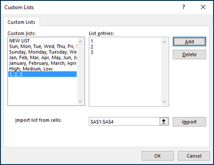
The items in the list that you have chosen will appear in the Custom lists panel.

Create a custom list from a cell range

Follow these steps:

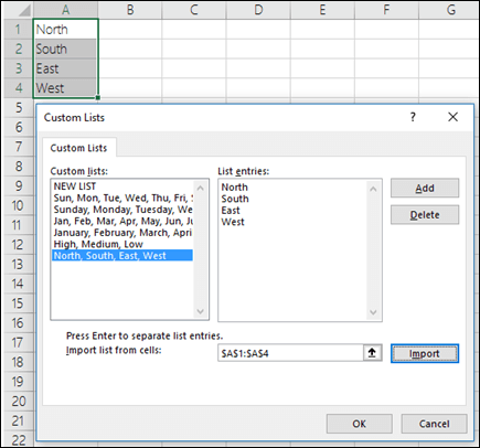
In a range of cells, enter the values that you want to sort or fill by, in the order that you want them, from top to bottom. Select the range of cells you just entered, and follow the previous instructions for displaying the Edit Custom Lists popup window.

In the Custom Lists popup window, verify that the cell reference of the list of items that you have chosen appears in the Import list from cells field, and then click Import.

The items in the list that you have chosen will appear in the Custom Lists panel.

Options > Advanced > General > Edit Custom Lists. For Excel 2007 click the Office Button > Excel Options > Popular > Edit Custom Lists.» loading=»lazy»>

Note: You can only create a custom list according to values, such as text, numbers, dates or times. You cannot create a custom list for formats such as cell color, font color, or an icon.

Follow these steps:

Follow the previous instructions for displaying the Edit Custom Lists dialog.

In the Custom Lists box, choose the list that you want to delete, and then click Delete.

Once you create a custom list, it is added to your computer registry, so that it is available for use in other workbooks. If you use a custom list when sorting data, it is also saved with the workbook, so that it can be used on other computers, including servers where your workbook might be published to Excel Services and you want to rely on the custom list for a sort.

However, if you open the workbook on another computer or server, you do not see the custom list that is stored in the workbook file in the Custom Lists popup window that is available from Excel Options, only from the Order column of the Sort dialog box. The custom list that is stored in the workbook file is also not immediately available for the Fill command.

If you prefer, add the custom list that is stored in the workbook file to the registry of the other computer or server and make it available from the Custom Lists popup window in Excel Options. From the Sort popup window, in the Order column, select Custom Lists to display the Custom Lists popup window, then select the custom list, and then click Add.

Need more help?

You can always ask an expert in the Excel Tech Community or get support in the Answers community.

Источник

Add or remove items from a drop-down list

After you create a drop-down list, you might want to add more items or delete items. In this article, we’ll show you how to do that depending on how the list was created.

Edit a drop-down list that’s based on an Excel Table

If you set up your list source as an Excel table, then all you need to do is add or remove items from the list, and Excel will automatically update any associated drop-downs for you.

To add an item, go to the end of the list and type the new item.

To remove an item, press Delete.

Tip: If the item you want to delete is somewhere in the middle of your list, right-click its cell, click Delete, and then click OK to shift the cells up.

Select the worksheet that has the named range for your drop-down list.

Do any of the following:

To add an item, go to the end of the list and type the new item.

To remove an item, press Delete.

Tip: If the item you want to delete is somewhere in the middle of your list, right-click its cell, click Delete, and then click OK to shift the cells up.

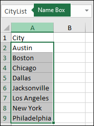
Go to Formulas > Name Manager.

In the Name Manager box, click the named range you want to update.

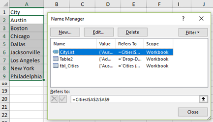
Click in the Refers to box, and then on your worksheet select all of the cells that contain the entries for your drop-down list.

Click Close, and then click Yes to save your changes.

Tip: If you don’t know what a named range is named, you can select the range and look for its name in the Name Box. To locate a named range, see Find named ranges.

Select the worksheet that has the data for your drop-down list.

Do any of the following:

To add an item, go to the end of the list and type the new item.

To remove an item, click Delete.

Tip: If the item you want to delete is somewhere in the middle of your list, right-click its cell, click Delete, and then click OK to shift the cells up.

On the worksheet where you applied the drop-down list, select a cell that has the drop-down list.

Go to Data > Data Validation.

On the Settings tab, click in the Source box, and then on the worksheet that has the entries for your drop-down list, select all of the cells containing those entries. You’ll see the list range in the Source box change as you select.

To update all cells that have the same drop-down list applied, check the Apply these changes to all other cells with the same settings box.

On the worksheet where you applied the drop-down list, select a cell that has the drop-down list.

Go to Data > Data Validation.

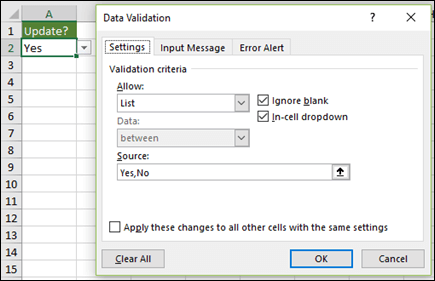
On the Settings tab, click in the Source box, and then change your list items as needed. Each item should be separated by a comma, with no spaces in between like this: Yes,No,Maybe.

To update all cells that have the same drop-down list applied, check the Apply these changes to all other cells with the same settings box.

After you update a drop-down list, make sure it works the way you want. For example, check to see if the cell is wide enough to show your updated entries.

If the list of entries for your drop-down list is on another worksheet and you want to prevent users from seeing it or making changes, consider hiding and protecting that worksheet. For more information about how to protect a worksheet, see Lock cells to protect them.

If you want to delete your drop-down list, see Remove a drop-down list.

To see a video about how to work with drop-down lists, see Create and manage drop-down lists.

Edit a drop-down list that’s based on an Excel Table

If you set up your list source as an Excel table, then all you need to do is add or remove items from the list, and Excel will automatically update any associated drop-downs for you.

To add an item, go to the end of the list and type the new item.

To remove an item, press Delete.

Tip: If the item you want to delete is somewhere in the middle of your list, right-click its cell, click Delete, and then click OK to shift the cells up.

Select the worksheet that has the named range for your drop-down list.

Do any of the following:

To add an item, go to the end of the list and type the new item.

To remove an item, press Delete.

Tip: If the item you want to delete is somewhere in the middle of your list, right-click its cell, click Delete, and then click OK to shift the cells up.

Go to Formulas > Name Manager.

In the Name Manager box, click the named range you want to update.

Click in the Refers to box, and then on your worksheet select all of the cells that contain the entries for your drop-down list.

Click Close, and then click Yes to save your changes.

Tip: If you don’t know what a named range is named, you can select the range and look for its name in the Name Box. To locate a named range, see Find named ranges.

Select the worksheet that has the data for your drop-down list.

Do any of the following:

To add an item, go to the end of the list and type the new item.

To remove an item, click Delete.

Tip: If the item you want to delete is somewhere in the middle of your list, right-click its cell, click Delete, and then click OK to shift the cells up.

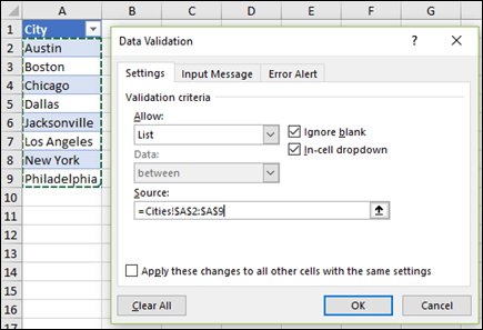
On the worksheet where you applied the drop-down list, select a cell that has the drop-down list.

Go to Data > Data Validation.

On the Settings tab, click in the Source box, and then on the worksheet that has the entries for your drop-down list, Select cell contents in Excel containing those entries. You’ll see the list range in the Source box change as you select.

To update all cells that have the same drop-down list applied, check the Apply these changes to all other cells with the same settings box.

On the worksheet where you applied the drop-down list, select a cell that has the drop-down list.

Go to Data > Data Validation.

On the Settings tab, click in the Source box, and then change your list items as needed. Each item should be separated by a comma, with no spaces in between like this: Yes,No,Maybe.

To update all cells that have the same drop-down list applied, check the Apply these changes to all other cells with the same settings box.

After you update a drop-down list, make sure it works the way you want. For example, check to see how to Change the column width and row height to show your updated entries.

If you want to delete your drop-down list, see Remove a drop-down list.

To see a video about how to work with drop-down lists, see Create and manage drop-down lists.

In Excel for the web, you can only edit a drop-down list where the source data has been entered manually.

Select the cells that have the drop-down list.

Go to Data > Data Validation.

On the Settings tab, click in the Source box. Then do one of the following:

If the Source box contains drop-down entries separated by commas, then type new entries or remove ones you don’t need. When you’re done, each entry should be separated by a comma, with no spaces. For example: Fruits,Vegetables,Meat,Deli.

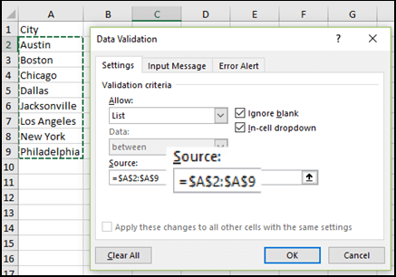
If the Source box contains a reference to a range of cells (for example, =$A$2:$A$5), click Cancel, and then add or remove entries from those cells. In this example, you’d add or remove entries in cells A2 through A5. If the list of entries ends up being longer or shorter than the original range, go back to the Settings tab and delete what’s in the Source box. Then click and drag to select the new range containing the entries.

If the Source box contains a named range, like Departments, then you need to change the range itself using a desktop version of Excel.

After you update a drop-down list, make sure it works the way you want. For example, check to see if the cell is wide enough to show your updated entries. If you want to delete your drop-down list, see Remove a drop-down list.

Need more help?

You can always ask an expert in the Excel Tech Community or get support in the Answers community.

Источник

Add or remove items from a drop-down list

Excel for Microsoft 365 Excel for Microsoft 365 for Mac Excel for the web Excel 2021 Excel 2021 for Mac Excel 2019 Excel 2019 for Mac Excel 2016 Excel 2016 for Mac Excel 2013 Excel 2010 Excel 2007 More…Less

After you create a drop-down list, you might want to add more items or delete items. In this article, we’ll show you how to do that depending on how the list was created.

Edit a drop-down list that’s based on an Excel Table

If you set up your list source as an Excel table, then all you need to do is add or remove items from the list, and Excel will automatically update any associated drop-downs for you.

To add an item, go to the end of the list and type the new item.
To remove an item, press Delete.

Tip: If the item you want to delete is somewhere in the middle of your list, right-click its cell, click Delete, and then click OK to shift the cells up.

Select the worksheet that has the named range for your drop-down list.
Do any of the following:
- To add an item, go to the end of the list and type the new item.
- To remove an item, press Delete.
  
  Tip: If the item you want to delete is somewhere in the middle of your list, right-click its cell, click Delete, and then click OK to shift the cells up.
Go to Formulas > Name Manager.
In the Name Manager box, click the named range you want to update.
Click in the Refers to box, and then on your worksheet select all of the cells that contain the entries for your drop-down list.
Click Close, and then click Yes to save your changes.

Tip: If you don’t know what a named range is named, you can select the range and look for its name in the Name Box. To locate a named range, see Find named ranges.

Select the worksheet that has the data for your drop-down list.
Do any of the following:
- To add an item, go to the end of the list and type the new item.
- To remove an item, click Delete.
  
  Tip: If the item you want to delete is somewhere in the middle of your list, right-click its cell, click Delete, and then click OK to shift the cells up.
On the worksheet where you applied the drop-down list, select a cell that has the drop-down list.
Go to Data > Data Validation.
On the Settings tab, click in the Source box, and then on the worksheet that has the entries for your drop-down list, select all of the cells containing those entries. You’ll see the list range in the Source box change as you select.
To update all cells that have the same drop-down list applied, check the Apply these changes to all other cells with the same settings box.

On the worksheet where you applied the drop-down list, select a cell that has the drop-down list.
Go to Data > Data Validation.
On the Settings tab, click in the Source box, and then change your list items as needed. Each item should be separated by a comma, with no spaces in between like this: Yes,No,Maybe.
To update all cells that have the same drop-down list applied, check the Apply these changes to all other cells with the same settings box.

After you update a drop-down list, make sure it works the way you want. For example, check to see if the cell is wide enough to show your updated entries.

If you want to delete your drop-down list, see Remove a drop-down list.

To see a video about how to work with drop-down lists, see Create and manage drop-down lists.

Edit a drop-down list that’s based on an Excel Table

If you set up your list source as an Excel table, then all you need to do is add or remove items from the list, and Excel will automatically update any associated drop-downs for you.

To add an item, go to the end of the list and type the new item.
To remove an item, press Delete.

Tip: If the item you want to delete is somewhere in the middle of your list, right-click its cell, click Delete, and then click OK to shift the cells up.

Select the worksheet that has the named range for your drop-down list.
Do any of the following:
- To add an item, go to the end of the list and type the new item.
- To remove an item, press Delete.
  
  Tip: If the item you want to delete is somewhere in the middle of your list, right-click its cell, click Delete, and then click OK to shift the cells up.
Go to Formulas > Name Manager.
In the Name Manager box, click the named range you want to update.
Click in the Refers to box, and then on your worksheet select all of the cells that contain the entries for your drop-down list.
Click Close, and then click Yes to save your changes.

Tip: If you don’t know what a named range is named, you can select the range and look for its name in the Name Box. To locate a named range, see Find named ranges.

Select the worksheet that has the data for your drop-down list.
Do any of the following:
- To add an item, go to the end of the list and type the new item.
- To remove an item, click Delete.
  
  Tip: If the item you want to delete is somewhere in the middle of your list, right-click its cell, click Delete, and then click OK to shift the cells up.
On the worksheet where you applied the drop-down list, select a cell that has the drop-down list.
Go to Data > Data Validation.
On the Settings tab, click in the Source box, and then on the worksheet that has the entries for your drop-down list, Select cell contents in Excel containing those entries. You’ll see the list range in the Source box change as you select.
To update all cells that have the same drop-down list applied, check the Apply these changes to all other cells with the same settings box.

On the worksheet where you applied the drop-down list, select a cell that has the drop-down list.
Go to Data > Data Validation.
On the Settings tab, click in the Source box, and then change your list items as needed. Each item should be separated by a comma, with no spaces in between like this: Yes,No,Maybe.
To update all cells that have the same drop-down list applied, check the Apply these changes to all other cells with the same settings box.

After you update a drop-down list, make sure it works the way you want. For example, check to see how to Change the column width and row height to show your updated entries.

If you want to delete your drop-down list, see Remove a drop-down list.

To see a video about how to work with drop-down lists, see Create and manage drop-down lists.

In Excel for the web, you can only edit a drop-down list where the source data has been entered manually.

Select the cells that have the drop-down list.
Go to Data > Data Validation.
On the Settings tab, click in the Source box. Then do one of the following:
- If the Source box contains drop-down entries separated by commas, then type new entries or remove ones you don’t need. When you’re done, each entry should be separated by a comma, with no spaces. For example: Fruits,Vegetables,Meat,Deli.
- If the Source box contains a reference to a range of cells (for example, =$A$2:$A$5), click Cancel, and then add or remove entries from those cells. In this example, you’d add or remove entries in cells A2 through A5. If the list of entries ends up being longer or shorter than the original range, go back to the Settings tab and delete what’s in the Source box. Then click and drag to select the new range containing the entries.
- If the Source box contains a named range, like Departments, then you need to change the range itself using a desktop version of Excel.

Need more help?

You can always ask an expert in the Excel Tech Community or get support in the Answers community.

How do you send an empty ArrayList in Java?

ArrayList clear() method is used to removes all of the elements from the list. The list will be empty after this call returns….ArrayList clear() – Empty ArrayList in Java

Method parameter – none.
Method returns – void.
Method throws – none.

How do you send an empty list?

Example 2

import java.util.*;
public class CollectionsEmptyListExample2 {
public static void main(String[] args) {
//Create an empty List.
List emptylist = Collections.emptyList();
System.out.println(“Created empty immutable list: “+emptylist);
//Try to add elements.
emptylist.add(“A”);

How do you delete lists on Android?

How to empty or clear ArrayList in Java

Clear arraylist with ArrayList. clear()
Clear arraylist with ArrayList. removeAll()
Difference between clear() vs removeAll() methods. As I said before, both methods empty an list.
Conclusion.

Источник

09-06-2012, 12:40 PM

#1

Registered User

Remove a List of Persons from a Larger List

Hello all,

I have a large list of customers, first and last names. I have another list of customer who need to be removed from the first list. Everyone on the second list is on the first list, but I can’t figure out a good way to remove them from the main list of people.

Any ideas? I looked into using VLOOKUP, is that the right direction?
09-06-2012, 12:45 PM

#2

Re: Remove a List of Persons from a Larger List

Personally I’d use COUNTIF to check which of the first list are also on the second list then filter the data to anything that isn’t zero and delete those rows.

If I’ve been of help, please hit the star
09-06-2012, 02:50 PM

#3

Registered User

Re: Remove a List of Persons from a Larger List

Originally Posted by Spencer101

Personally I’d use COUNTIF to check which of the first list are also on the second list then filter the data to anything that isn’t zero and delete those rows.

That sounds like exactly what I want! I’m a sorry excuse of an excel user, so I’ve never used COUNTIF. From what I see, it only identifies weather or not a thing exists in a range, not where/what it is. Would you mind explaining your idea a little further? I really appreciate your help.
09-06-2012, 02:58 PM

#4

Re: Remove a List of Persons from a Larger List

Have a look at the attached.

Sheet 1 is your «main list»
Sheet 2 is your list to check against.

Column A on Sheet 1 holds the main list of names
Column A on Sheet 2 holds the list of names to be checked against.
Column B on Sheet 1 holds the results of the COUNTIF

So the COUNTIF formula compares the value in column A against the whole list on Sheet 2. If it finds any instances it will show how many. If it doesn’t it will show zero.

So all you have to do is apply the auto filter on column B of Sheet 1 to show anything other than zero and delete those rows.

On your workbook you will obviously have to alter the ranges to fit your dataset.

Let me know if you need anything more on this
09-07-2012, 03:37 PM

#5

Registered User

Re: Remove a List of Persons from a Larger List

Yes! That’s it! Thank you, you saved me so much headache!
09-07-2012, 03:59 PM

#6

Re: Remove a List of Persons from a Larger List

Not a problem. Glad to help!

Источник

I have two lists in excel, let’s call them B and A. if there is an email in list A that matches an email form list A I need to delete it. I could do this manually but that would be weeks of work. There’s got to be a way to get excel to do it for me.

EDIT/UPDATE

here is a pic of situation/problem

I know nothing about Excel, so the first thing I would like to do is to remove any duplicates from within the lists themselves. but then I would also like any contacts/emails from list B that has a duplicate in list A to be removed. for example, if the email John@John.com is in list B and there is also a John@john.com in list A, I want to remove John@john.com from list B

asked Feb 20, 2018 at 20:59

One way is to use vlookup (or match/index if you have millions of emails, it’s faster). Add a column in the sheet with the emails to be managed called «Keep», add a formula to set it to TRUE if the email is in the inactive list, or false if it’s not. You can then filter the list to only the rows where Keep is FALSE, and delete those rows. One tip with vlookup — if you highlight the range of inactive emails and name the range (in the screenshot below, click in the top left where it says B2 and type in «Inactive»), then you can use that name in the vlookup formula, which makes life easier. Really needs to be a video

E.g.

answered Feb 20, 2018 at 21:46

Источник

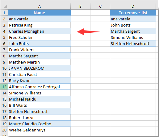
Предположим, у вас есть два списка данных, как показано на скриншоте слева. Теперь вам нужно удалить или исключить имена в столбце A, если имя существует в столбце D. Как этого добиться? А что, если два списка находятся на двух разных листах? Эта статья предлагает вам два метода.

Исключить значения в одном списке из другого с помощью формулы

Быстро исключайте значения в одном списке из другого с помощью Kutools for Excel

Исключить значения в одном списке из другого с помощью формулы

Для этого вы можете применить следующие формулы. Пожалуйста, сделайте следующее.

1. Выберите пустую ячейку, которая находится рядом с первой ячейкой списка, который вы хотите удалить, затем введите формулу. = СЧЁТЕСЛИ ($ D $ 2: $ D $ 6; A2) в панель формул, а затем нажмите Enter ключ. Смотрите скриншот:

Внимание: В формуле $ D $ 2: $ D $ 6 — это список, на основе которого вы удаляете значения, A2 — это первая ячейка списка, который вы собираетесь удалить. Пожалуйста, измените их по своему усмотрению.

2. Продолжая выбирать ячейку результата, перетащите маркер заполнения вниз, пока он не достигнет последней ячейки списка. Смотрите скриншот:

3. Продолжайте выбирать список результатов, затем щелкните Данные > Сортировка от А до Я.

Затем вы можете увидеть, что список отсортирован, как показано на скриншоте ниже.

4. Теперь выберите все строки имен с результатом 1, щелкните правой кнопкой мыши выбранный диапазон и нажмите Удалить чтобы удалить их.

Теперь вы исключили значения из одного списка на основе другого.

Внимание: Если «список для удаления» находится в диапазоне A2: A6 другого листа, такого как Sheet2, примените эту формулу = IF (ISERROR (VLOOKUP (A2; Sheet2! $ A $ 2: $ A $ 6,1; FALSE)), «Сохранить», «Удалить») получить все Сохранить и Удалить результатов, отсортируйте список результатов от A до Z, а затем вручную удалите все строки имен, содержащие результат удаления на текущем листе.

Быстро исключайте значения в одном списке из другого с помощью Kutools for Excel

Этот раздел будет рекомендовать Выберите одинаковые и разные ячейки полезности Kutools for Excel чтобы решить эту проблему. Пожалуйста, сделайте следующее.

1. Нажмите Кутулс > Выберите > Выберите одинаковые и разные ячейки. Смотрите скриншот:

2. в Выберите одинаковые и разные ячейки диалоговое окно, вам необходимо:

2.1 Выберите список, из которого вы удалите значения в Найдите значения в коробка;
2.2 Выберите список, значения которого вы удалите, на основе Согласно информации коробка;
2.3 выберите Однокамерная вариант в на основании раздел;
2.4 Щелкните значок OK кнопка. Смотрите скриншот:

3. Затем появляется диалоговое окно, в котором указывается, сколько ячеек было выбрано, нажмите OK кнопку.

4. Теперь значения в столбце A выбираются, если они существуют в столбце D. Вы можете нажать кнопку Удалить клавишу, чтобы удалить их вручную.

Если вы хотите получить бесплатную пробную версию (30-день) этой утилиты, пожалуйста, нажмите, чтобы загрузить это, а затем перейдите к применению операции в соответствии с указанными выше шагами.

Быстро исключайте значения в одном списке из другого с помощью Kutools for Excel

Статьи по теме:

Как исключить определенную ячейку или область из печати в Excel?
Как исключить ячейки в столбце из суммы в Excel?
Как найти минимальное значение в диапазоне без нулевого значения в Excel?

Лучшие инструменты для работы в офисе

Kutools for Excel Решит большинство ваших проблем и повысит вашу производительность на 80%

Снова использовать: Быстро вставить сложные формулы, диаграммы и все, что вы использовали раньше; Зашифровать ячейки с паролем; Создать список рассылки и отправлять электронные письма …
Бар Супер Формулы (легко редактировать несколько строк текста и формул); Макет для чтения (легко читать и редактировать большое количество ячеек); Вставить в отфильтрованный диапазон…
Объединить ячейки / строки / столбцы без потери данных; Разделить содержимое ячеек; Объединить повторяющиеся строки / столбцы… Предотвращение дублирования ячеек; Сравнить диапазоны…
Выберите Дубликат или Уникальный Ряды; Выбрать пустые строки (все ячейки пустые); Супер находка и нечеткая находка во многих рабочих тетрадях; Случайный выбор …
Точная копия Несколько ячеек без изменения ссылки на формулу; Автоматическое создание ссылок на несколько листов; Вставить пули, Флажки и многое другое …
Извлечь текст, Добавить текст, Удалить по позиции, Удалить пробел; Создание и печать промежуточных итогов по страницам; Преобразование содержимого ячеек в комментарии…
Суперфильтр (сохранять и применять схемы фильтров к другим листам); Расширенная сортировка по месяцам / неделям / дням, периодичности и др .; Специальный фильтр жирным, курсивом …
Комбинируйте книги и рабочие листы; Объединить таблицы на основе ключевых столбцов; Разделить данные на несколько листов; Пакетное преобразование xls, xlsx и PDF…
Более 300 мощных функций. Поддерживает Office/Excel 2007-2021 и 365. Поддерживает все языки. Простое развертывание на вашем предприятии или в организации. Полнофункциональная 30-дневная бесплатная пробная версия. 60-дневная гарантия возврата денег.

Вкладка Office: интерфейс с вкладками в Office и упрощение работы

Включение редактирования и чтения с вкладками в Word, Excel, PowerPoint, Издатель, доступ, Visio и проект.
Открывайте и создавайте несколько документов на новых вкладках одного окна, а не в новых окнах.
Повышает вашу продуктивность на 50% и сокращает количество щелчков мышью на сотни каждый день!

Комментарии (16)

Оценок пока нет. Оцените первым!

Источник

In this article, we will show you how to create, delete, and use a Custom List in Microsoft Excel. The Custom List feature is useful for the users who have to type a specific list in every Excel spreadsheet. If this is the case with you, this post will help you save time.

How can an Excel Custom List make your work easier and faster?

Excel has some built-in Lists that include names of the days and names of the months. You cannot edit or delete these built-in lists. Let’s understand the benefits of these built-in lists. Let’s say, you have to prepare data for weekly analysis of rainfall. In this data, you have to enter days’ names. If you do not know the usage of the Custom Lists, you have to type the days’ names manually which will take time. On the other hand, the user who knows the usage of the Custom List will type only the name of the day, say, Monday, and drag the cell. After that, Excel will fill all the cells with the days’ names in the correct order. This is how a Custom List makes your work easier and faster.

Can you create your own Custom List in Excel?

Yes, you can create your own Custom List in Excel. You can find the respective option int he Advanced category. From here, you need to use the Edit Custom Lists option to start creating the list. In this article, we have explained the process of creating, deleting, and using a Custom List in Microsoft Excel.

The steps to create a Custom List in Microsoft Excel are as follows:

Launch Microsoft Excel and create a Custom List.
Go to “File > Options.”
Select the Advanced category from the left pane.
Click on the Edit Custom Lists button.
Import your Custom List from the Excel worksheet.
Click OK.

Let’s see these steps in detail.

1] Launch Microsoft Excel and create a Custom List. Here, we have created a sample list of names of some states of the USA.

2] Click on the File menu and then select Options. This will open the Excel Options window.

3] In the Excel Options window, select the Advanced category from the left side. Now, scroll down the right side and click on the Edit Custom Lists button. You will find this button in the General section.

4] Now, click inside the box next to the Import list from cells. After that, select the range of the cells to insert the list. See the below screenshot.

5] Click on the Import button. When you click on the Import button, your list will be added to the Custom LIsts menu. Now, click OK and exit the Excel Options window.

You can also create a Custom List from the List Entries box. For this, first, type your Custom List in the List entries box and then click on the Add button. This will add your list to the Custom Lists menu.

How do I delete a Custom List in Excel?

Deleting a Custom List is easy. You need to select the list that you want to delete and then click on the Delete button. We have explained the steps for the same above in this article. No matter whether you have one or multiple lists in your spreadsheet, you need to follow the same steps to delete them all.

We have learned how to create a Custom List in Excel. Now, let’s see how to delete a Custom List in Excel. As we have described previously in this article, you cannot delete the built-in list in Excel. But you can delete those you have created.

To delete a Custom List in Excel, go to “File > Options > Advanced > Edit Custom Lists.” After that, select the list that you want to delete from the Custom Lists menu and then click on the Delete button. A popup window will appear showing you a message “List will be permanently deleted.” Click OK. This will delete the Custom List from Excel.

How to use a Custom List in Excel

Now, let’s talk about how to use a Custom List in Excel.

Follow the instructions below:

Click on a cell in the document in which you want to insert your Custom List.
Type the name from which your Custom List starts.
Drag the cells to the bottom. This will fill up all the remaining entries automatically.

What are the two ways to create a Custom List?

The following are the two ways to create a Custom List in Microsoft Excel:

By using the Import option.
By using the List Entries box.

We have explained both of these methods above in this article.

That’s it.

Read next:

How to create a Combination Chart in Microsoft Excel.
How to create a drop-down list in Excel and Google Sheets.

Источник

Deleting unused blank rows from a sheet can help you reduce file size significantly and make your dashboard cleaner. In this article we will learn the ways you can delete unused rows from a worksheet fast.

We will discuss these methods for deleting rows in this article:

Literally Deleting Blank Rows at the Bottom of the Excel Sheet

Delete Unused Rows Within Used Range

Reset Last Used Range

Delete Unused Rows So That They Don’t Show (Hide Them).

How To Delete Extra Blank Rows From Sheets?

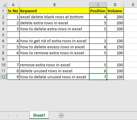
Here we have a data table. The rows below the 12th row are unused and I would like to delete these rows and the data if they contain any. To do so, I select the 13th row and press CTRL+SHIFT +DOWN Arrow key. Keep this combination pressed until you reach the last row in the sheet.

Now press the CTRL+SHIFT+SPACE key combination. This will select the entire row of selected cells.

Now press CTRL+ — (CTRL and Minus) key combination. This will delete the entire rows.

Learn 50 Excel Shortcuts to Increase Your Productivity.

How To Get Rid of Extra Blank Rows Within The Table?

In the above table, we can see some blank rows. In this example, we have only 2 blank rows, which can be deleted manually. In real data you may have thousands of rows with hundreds of random unused rows. In such cases deleting blank rows can be a major issue. But don’t worry, we got it covered. You can delete unused rows in one go.

Follow these steps to delete all unused rows from the data table:

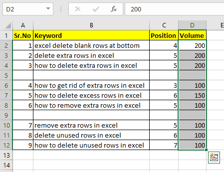
Select the entire main column by which you want to delete blank rows. I select the D column in Table because if there is no volume of the keyword, that row is useless to me.

Now press CTRL+G combination to open the Go-To dialog.

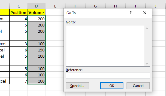
You can see a «Special» button at the bottom left corner. Click on it.

This is Go To special dialog. You can open it from Home —> Editing —> Find —> Select —> Go To Special option too.

Find the «Blank» option button. Click on it and hit OK.

Excel will select the blank cells in that column.

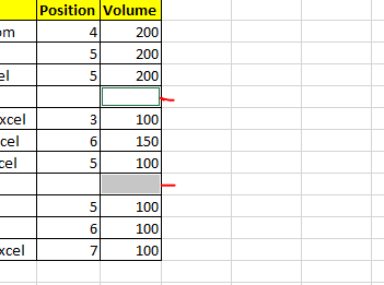
Now hit CTRL+SHIFT+SPACE to select entire rows of selected cells. It will select the entire row. Now hit the CTRL + — key combination to delete the selected rows.

Resetting the Last Used Range

It happens many times that we go far down in the sheet to do some rough work. After doing that rough work in a cell or row or column, we delete the data. Now we expect excel to forget that. But excel doesn’t forget easily.

Let’s say if you write «Hi» in cell A10000. You go back to cell A2 and write something there, say «Hello Exceltip.com». Now go back to A10000 and delete the content from there. Back to A1.

Now if you press CTRL+END , the cursor will move to cell A1000. Even if you delete that row. Nothing will work. Excel will remember the cell and it will consider it in used range.

To reset it, we use this code line in VBA.

Worksheet.UsedRange

Here’s how you use it.

Press Alt + F11 to open the VB Editor.

Write this in any module or worksheet.

Sub test()
  ActiveSheet.UsedRange
End Sub

Run this and you will have your used range reset. Now if you hit CTRL+End shortcut. It will take you to the last cell that has data in it.

Alternative to sub

You can also use the immediate window to reset the used range and ignore used rows and columns.

To open an immediate window, go to the view menu and find an immediate window. Click on it and you will have it below in VBE. The immediate window is used to debug code but you can use it to run small chunks of code without saving them.

In the Immediate window, write this line «Activesheet.usedrange» and hit the enter button. Nothing will reflect this but the work is done. Go to the activesheet.

Make unused rows invisible

If you want to delete the unused rows so that they aren’t visible for the sake of the dashboard. Then deleting the rows won’t work in this new version. Every time you delete rows, new rows will take place (only for viewing, they don’t have weight).

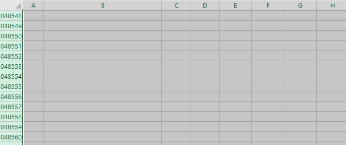
So to delete rows at the bottom of the sheet, so that they don’t appear on the sheet, we hide them.

Select the first empty cell after the used range and use the shortcut CTRL+SHIFT+DOWN key to select the entire column below the used range. Now hit CTRL+SHIFT+SPACE to select the entire row.

Right now click on the selected rows.

Find the hide option. Click on it. This will hide all the rows below the used range. Now no one can edit in those rows.

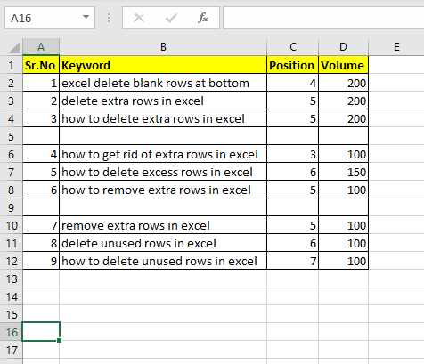
You can see that all the unused at the bottom of the sheet are gone.

Related Article

Delete drop down list in Excel: The dropdown list is used to restrict the user to input data and gives the option to select from the list. We need to delete or remove the dropdown list as the user will be able to input any data instead of choosing from a list.

Deleting All Cell Comments in Excel 2016 : Comments in Excel to remind ourselves and inform someone else about what the cell contains. To add a comment in a cell, Excel 2016 provides the insert Comment function. After inserting the comment it is displayed with little red triangles.

How to Delete only Filtered Rows without the Hidden Rows in Excel: Many of you are asking how to delete the selected rows without disturbing the other rows. We will use the Find & Select option in Excel.

How to Delete Sheets Without Confirmation Prompts Using VBA In Excel: There are times when we have to create or add sheets and later on we find no use of that sheet, hence we get the need to delete sheets quickly from the workbook. This

Popular Articles:

50 Excel Shortcuts to Increase Your Productivity | Get faster at your task. These 50 shortcuts will make you work even faster on Excel.

How to use Excel VLOOKUP Function| This is one of the most used and popular functions of excel that is used to lookup value from different ranges and sheets.

How to use the Excel COUNTIF Function| Count values with conditions using this amazing function. You don’t need to filter your data to count specific values. Countif function is essential to prepare your dashboard.

How to Use SUMIF Function in Excel | This is another dashboard essential function. This helps you sum up values on specific conditions.

Источник

Create or delete a custom list for sorting and filling data

Need more help?

Add or remove items from a drop-down list

Edit a drop-down list that’s based on an Excel Table

Edit a drop-down list that’s based on an Excel Table

Need more help?

Edit a drop-down list that’s based on an Excel Table

Edit a drop-down list that’s based on an Excel Table

Need more help?

See Also

Need more help?

How do I remove an item from an ArrayList?

How do you send an empty ArrayList in Java?

How do you delete lists on Android?

Remove a List of Persons from a Larger List

Re: Remove a List of Persons from a Larger List

Re: Remove a List of Persons from a Larger List

Re: Remove a List of Persons from a Larger List

Re: Remove a List of Persons from a Larger List

Re: Remove a List of Persons from a Larger List

Исключить значения в одном списке из другого с помощью формулы

Быстро исключайте значения в одном списке из другого с помощью Kutools for Excel

Быстро исключайте значения в одном списке из другого с помощью Kutools for Excel

Статьи по теме:

Лучшие инструменты для работы в офисе

Kutools for Excel Решит большинство ваших проблем и повысит вашу производительность на 80%

Вкладка Office: интерфейс с вкладками в Office и упрощение работы

How can an Excel Custom List make your work easier and faster?

Can you create your own Custom List in Excel?

How do I delete a Custom List in Excel?

How to use a Custom List in Excel

What are the two ways to create a Custom List?

How To Delete Extra Blank Rows From Sheets?

How To Get Rid of Extra Blank Rows Within The Table?

Resetting the Last Used Range

Make unused rows invisible