Remove duplicates in rows excel - Word и Excel - помощь в работе с программами

Find and remove duplicates

Excel for Microsoft 365 Excel 2021 Excel 2019 Excel 2016 Excel 2013 Excel 2010 Excel 2007 Excel Starter 2010 More…Less

Sometimes duplicate data is useful, sometimes it just makes it harder to understand your data. Use conditional formatting to find and highlight duplicate data. That way you can review the duplicates and decide if you want to remove them.

Select the cells you want to check for duplicates.

Note: Excel can’t highlight duplicates in the Values area of a PivotTable report.
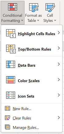
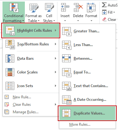
Click Home > Conditional Formatting > Highlight Cells Rules > Duplicate Values.
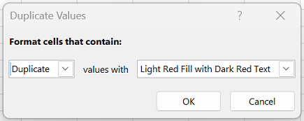
In the box next to values with, pick the formatting you want to apply to the duplicate values, and then click OK.

Remove duplicate values

When you use the Remove Duplicates feature, the duplicate data will be permanently deleted. Before you delete the duplicates, it’s a good idea to copy the original data to another worksheet so you don’t accidentally lose any information.

Select the range of cells that has duplicate values you want to remove.
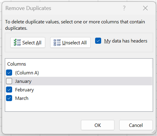
Click Data > Remove Duplicates, and then Under Columns, check or uncheck the columns where you want to remove the duplicates.

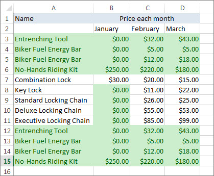
For example, in this worksheet, the January column has price information I want to keep.

So, I unchecked January in the Remove Duplicates box.
Click OK.

Note: The counts of duplicate and unique values given after removal may include empty cells, spaces, etc.

Need more help?

Источник

Duplicate values in your data can be a big problem! It can lead to substantial errors and over estimate your results.

But finding and removing them from your data is actually quite easy in Excel.

In this tutorial, we are going to look at 7 different methods to locate and remove duplicate values from your data.

Video Tutorial

What Is A Duplicate Value?

Duplicate values happen when the same value or set of values appear in your data.

For a given set of data you can define duplicates in many different ways.

In the above example, there is a simple set of data with 3 columns for the Make, Model and Year for a list of cars.

The first image highlights all the duplicates based only on the Make of the car.
The second image highlights all the duplicates based on the Make and Model of the car. This results in one less duplicate.
The second image highlights all the duplicates based on all columns in the table. This results in even less values being considered duplicates.

The results from duplicates based on a single column vs the entire table can be very different. You should always be aware which version you want and what Excel is doing.

Find And Remove Duplicate Values With The Remove Duplicates Command

Removing duplicate values in data is a very common task. It’s so common, there’s a dedicated command to do it in the ribbon.

Select a cell inside the data which you want to remove duplicates from and go to the Data tab and click on the Remove Duplicates command.

Excel will then select the entire set of data and open up the Remove Duplicates window.

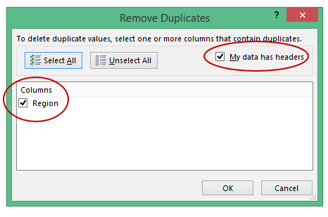
You then need to tell Excel if the data contains column headers in the first row. If this is checked, then the first row of data will be excluded when finding and removing duplicate values.
You can then select which columns to use to determine duplicates. There are also handy Select All and Unselect All buttons above you can use if you’ve got a long list of columns in your data.

When you press OK, Excel will then remove all the duplicate values it finds and give you a summary count of how many values were removed and how many values remain.

This command will alter your data so it’s best to perform the command on a copy of your data to retain the original data intact.

Find And Remove Duplicate Values With Advanced Filters

There is also another way to get rid of any duplicate values in your data from the ribbon. This is possible from the advanced filters.

Select a cell inside the data and go to the Data tab and click on the Advanced filter command.

This will open up the Advanced Filter window.

You can choose to either to Filter the list in place or Copy to another location. Filtering the list in place will hide rows containing any duplicates while copying to another location will create a copy of the data.
Excel will guess the range of data, but you can adjust it in the List range. The Criteria range can be left blank and the Copy to field will need to be filled if the Copy to another location option was chosen.
Check the box for Unique records only.

Press OK and you will eliminate the duplicate values.

Advanced filters can be a handy option for getting rid of your duplicate values and creating a copy of your data at the same time. But advanced filters will only be able to perform this on the entire table.

Find And Remove Duplicate Values With A Pivot Table

Pivot tables are just for analyzing your data, right?

You can actually use them to remove duplicate data as well!

You won’t actually be removing duplicate values from your data with this method, you will be using a pivot table to display only the unique values from the data set.

First, create a pivot table based on your data. Select a cell inside your data or the entire range of data ➜ go to the Insert tab ➜ select PivotTable ➜ press OK in the Create PivotTable dialog box.

With the new blank pivot table add all fields into the Rows area of the pivot table.

You will then need to change the layout of the resulting pivot table so it’s in a tabular format. With the pivot table selected, go to the Design tab and select Report Layout. There are two options you will need to change here.

Select the Show in Tabular Form option.
Select the Repeat All Item Labels option.

You will also need to remove any subtotals from the pivot table. Go to the Design tab ➜ select Subtotals ➜ select Do Not Show Subtotals.

You now have a pivot table that mimics a tabular set of data!

Pivot tables only list unique values for items in the Rows area, so this pivot table will automatically remove any duplicates in your data.

Find And Remove Duplicate Values With Power Query

Power Query is all about data transformation, so you can be sure it has the ability to find and remove duplicate values.

Select the table of values which you want to remove duplicates from ➜ go to the Data tab ➜ choose a From Table/Range query.

Remove Duplicates Based On One Or More Columns

With Power Query, you can remove duplicates based on one or more columns in the table.

You need to select which columns to remove duplicates based on. You can hold Ctrl to select multiple columns.

Right click on the selected column heading and choose Remove Duplicates from the menu.

You can also access this command from the Home tab ➜ Remove Rows ➜ Remove Duplicates.

= Table.Distinct(#"Previous Step", {"Make", "Model"})

If you look at the formula that’s created, it is using the Table.Distinct function with the second parameter referencing which columns to use.

Remove Duplicates Based On The Entire Table

To remove duplicates based on the entire table, you could select all the columns in the table then remove duplicates. But there is a faster method that doesn’t require selecting all the columns.

There is a button in the top left corner of the data preview with a selection of commands that can be applied to the entire table.

Click on the table button in the top left corner ➜ then choose Remove Duplicates.

= Table.Distinct(#"Previous Step")

If you look at the formula that’s created, it uses the same Table.Distinct function with no second parameter. Without the second parameter, the function will act on the whole table.

Keep Duplicates Based On A Single Column Or On The Entire Table

In Power Query, there are also commands for keeping duplicates for selected columns or for the entire table.

Follow the same steps as removing duplicates, but use the Keep Rows ➜ Keep Duplicates command instead. This will show you all the data that has a duplicate value.

Find And Remove Duplicate Values Using A Formula

You can use a formula to help you find duplicate values in your data.

First you will need to add a helper column that combines the data from any columns which you want to base your duplicate definition on.

= [@Make] & [@Model] & [@Year]

The above formula will concatenate all three columns into a single column. It uses the ampersand operator to join each column.

= TEXTJOIN("", FALSE , CarList[@[Make]:[Year]])

If you have a long list of columns to combine, you can use the above formula instead. This way you can simply reference all the columns as a single range.

You will then need to add another column to count the duplicate values. This will be used later to filter out rows of data that appear more than once.

= COUNTIFS($E$3:E3, E3)

Copy the above formula down the column and it will count the number of times the current value appears in the list of values above.

If the count is 1 then it’s the first time the value is appearing in the data and you will keep this in your set of unique values. If the count is 2 or more then the value has already appeared in the data and it is a duplicate value which can be removed.

Add filters to your data list.

Go to the Data tab and select the Filter command.
Use the keyboard shortcut Ctrl + Shift + L.

Now you can filter on the Count column. Filtering on 1 will produce all the unique values and remove any duplicates.

You can then select the visible cells from the resulting filter to copy and paste elsewhere. Use the keyboard shortcut Alt + ; to select only the visible cells.

Find And Remove Duplicate Values With Conditional Formatting

With conditional formatting, there’s a way to highlight duplicate values in your data.

Just like the formula method, you need to add a helper column that combines the data from columns. The conditional formatting doesn’t work with data across rows, so you’ll need this combined column if you want to detect duplicates based on more than one column.

Then you need to select the column of combined data.

To create the conditional formatting, go to the Home tab ➜ select Conditional Formatting ➜ Highlight Cells Rules ➜ Duplicate Values.

This will open up the conditional formatting Duplicate Values window.

You can select to either highlight Duplicate or Unique values.
You can also choose from a selection of predefined cell formats to highlight the values or create your own custom format.

Warning: The previous methods to find and remove duplicates considers the first occurrence of a value as a duplicate and will leave it intact. However, this method will highlight the first occurrence and will not make any distinction.

With the values highlighted, you can now filter on either the duplicate or unique values with the filter by color option. Make sure to add filters to your data. Go to the Data tab and select the Filter command or use the keyboard shortcut Ctrl + Shift + L.

Click on the filter toggle.
Select Filter by Color in the menu.
Filter on the color used in the conditional formatting to select duplicate values or filter on No Fill to select unique values.

You can then select just the visible cells with the keyboard shortcut Alt + ;.

Find And Remove Duplicate Values Using VBA

There is a built in command in VBA for removing duplicates within list objects.

Sub RemoveDuplicates() Dim DuplicateValues As Range Set DuplicateValues = ActiveSheet.ListObjects("CarList").Range DuplicateValues.RemoveDuplicates Columns:=Array(1, 2, 3), Header:=xlYes End Sub

The above procedure will remove duplicates from an Excel table named CarList.

Columns:=Array(1, 2, 3)

The above part of the procedure will set which columns to base duplicate detection on. In this case it will be on the entire table since all three columns are listed.

Header:=xlYes

The above part of the procedure tells Excel the first row in our list contains column headings.

You will want to create a copy of your data before running this VBA code, as it can’t be undone after the code runs.

Conclusions

Duplicate values in your data can be a big obstacle to a clean data set.

Thankfully, there are many options in Excel to easily remove those pesky duplicate values.

So, what’s your go to method to remove duplicates?

About the Author

John MacDougall

John is a Microsoft MVP and qualified actuary with over 15 years of experience. He has worked in a variety of industries, including insurance, ad tech, and most recently Power Platform consulting. He is a keen problem solver and has a passion for using technology to make businesses more efficient.

Источник

Watch Video – How to Find and Remove Duplicates in Excel

With a lot of data…comes a lot of duplicate data.

Duplicates in Excel can cause a lot of troubles. Whether you import data from a database, get it from a colleague, or collate it yourself, duplicates data can always creep in. And if the data you are working with is huge, then it becomes really difficult to find and remove these duplicates in Excel.

In this tutorial, I’ll show you how to find and remove duplicates in Excel.

FIND and HIGHLIGHT Duplicates in Excel.
- Find and Highlight Duplicates in a Single Column.
- Find and Highlight Duplicates in Multiple Columns.
- Find and Highlight Duplicate Rows.
REMOVE Duplicates in Excel.
- Remove Duplicates from a Single Column.
- Remove Duplicates from Multiple Columns.
- Remove Duplicate Rows.

Find and Highlight Duplicates in Excel

Duplicates in Excel can come in many forms. You can have it in a single column or multiple columns. There may also be a duplication of an entire row.

Finding and Highlight Duplicates in a Single Column in Excel

Conditional Formatting makes it simple to highlight duplicates in Excel.

Here is how to do it:

Select the data in which you want to highlight the duplicates.

Go to Home –> Conditional Formatting –> Highlight Cell Rules –> Duplicate Values.

In the Duplicate Values dialog box, select Duplicate in the drop down on the left, and specify the format in which you want to highlight the duplicate values. You can choose from the ready-made format options (in the drop down on the right), or specify your own format.

This will highlight all the values that have duplicates.

Quick Tip: Remember to check for leading or trailing spaces. For example, “John” and “John ” are considered different as the latter has an extra space character in it. A good idea would be to use the TRIM function to clean your data.

Finding and Highlight Duplicates in Multiple Columns in Excel

If you have data that spans multiple columns and you need to look for duplicates in it, the process is exactly the same as above.

Here is how to do it:

Select the data.
Go to Home –> Conditional Formatting –> Highlight Cell Rules –> Duplicate Values.
In the Duplicate Values dialog box, select Duplicate in the drop down on the left, and specify the format in which you want to highlight the duplicate values.
This will highlight all the cells that have duplicates value in the selected data set.

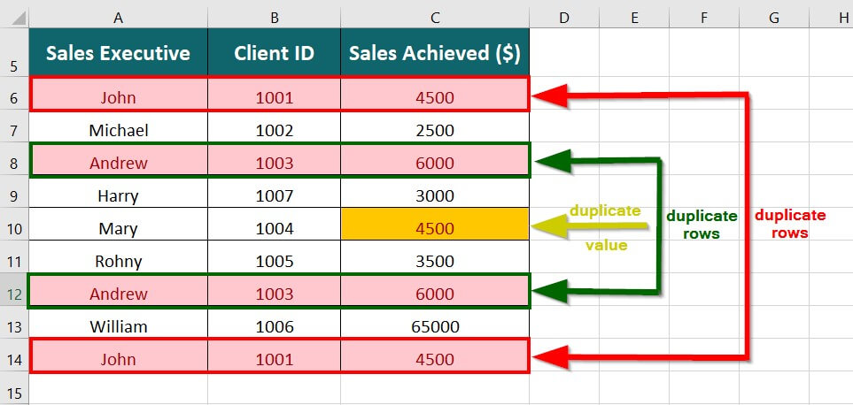
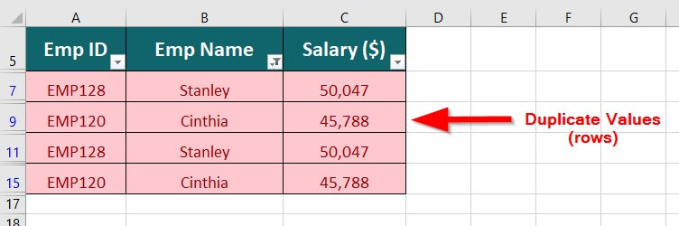
Finding and Highlighting Duplicate Rows in Excel

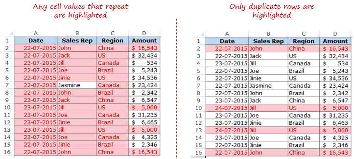
Finding duplicate data and finding duplicate rows of data are 2 different things. Have a look:

Finding duplicate rows is a bit more complex than finding duplicate cells.

Here are the steps:

In an adjacent column, use the following formula:
=A2&B2&C2&D2
Drag this down for all the rows. This formula combines all the cell values as a single string. (You can also use the CONCATENATE function to combine text strings)

By doing this, we have created a single string for each row. If there are duplicate rows in this dataset, then these strings would be exactly the same for it.

Now that we have the combined strings for each row, we can use conditional formatting to highlight duplicate strings. A highlighted string implies that the row has a duplicate.

Here are the steps to highlight duplicate strings:

Select the range that has the combined strings (E2:E16 in this example).
Go to Home –> Conditional Formatting –> Highlight Cell Rules –> Duplicate Values.
In the Duplicate Values dialog box, make sure Duplicate is selected and then specify the color in which you want to highlight the duplicate values.

This would highlight the duplicate values in column E.

In the above approach, we have highlighted only the strings that we created.

But what if you want to highlight all the duplicate rows (instead of highlighting cells in one single column)?

Here are the steps to highlight duplicate rows:

In an adjacent column, use the following formula:
=A2&B2&C2&D2
Drag this down for all the rows. This formula combines all the cell values as a single string.

Select the data A2:D16.
With the data selected, go to Home –> Conditional Formatting –> New Rule.

In the ‘New Formatting Rule’ dialog box, click on ‘Use a formula to determine which cells to format’.
In the field below, use the following COUNTIF function:
=COUNTIF($E$2:$E$16,$E2)>1

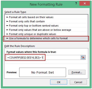
Select the format and click OK.

This formula would highlight all the rows that have a duplicate.

Remove Duplicates in Excel

In the above section, we learned how to find and highlight duplicates in excel. In this section, I will show you how to get rid of these duplicates.

Remove Duplicates from a Single Column in Excel

If you have the data in a single column and you want to remove all the duplicates, here are the steps:

Select the data.
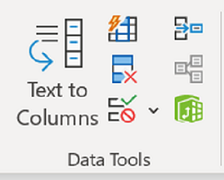
Go to Data –> Data Tools –> Remove Duplicates.
In the Remove Duplicates dialog box:
- If your data has headers, make sure the ‘My data has headers’ option is checked.
- Make sure the column is selected (in this case there is only one column).

Click OK.

This would remove all the duplicate values from the column, and you would have only the unique values.

CAUTION: This alters your data set by removing duplicates. Make sure you have a back-up of the original data set. If you want to extract the unique values at some other location, copy this dataset to that location and then use the above-mentioned steps. Alternatively, you can also use Advanced Filter to extract unique values to some other location.

Remove Duplicates from Multiple Columns in Excel

Suppose you have the data as shown below:

In the above data, row #2 and #16 have the exact same data for Sales Rep, Region, and Amount, but different dates (same is the case with row #10 and #13). This could be an entry error where the same entry has been recorded twice with different dates.

To delete the duplicate row in this case:

Select the data.
Go to Data –> Data Tools –> Remove Duplicates.
In the Remove Duplicates dialog box:
- If your data has headers, make sure the ‘My data has headers’ option is checked.
- Select all the columns except the Date column.

Click OK.

This would remove the 2 duplicate entries.

NOTE: This keeps the first occurrence and removes all the remaining duplicate occurrences.

Remove Duplicate Rows in Excel

To delete duplicate rows, here are the steps:

Select the entire data.
Go to Data –> Data Tools –> Remove Duplicates.
In the Remove Duplicates dialog box:
- If your data has headers, make sure the ‘My data has headers’ option is checked.
- Select all the columns.

Click OK.

Use the above-mentioned techniques to clean your data and get rid of duplicates.

You May Also Like the Following Excel Tutorials:

10 Ways to Clean Data in Excel Spreadsheets.
Remove Leading and Trailing Spaces in Excel.
24 Daily Excel Issues and their Quick Fixes.
How to Find Merged Cells in Excel.

Источник

Excel spreadsheets continue to represent a key tool for data storage and visualization. Functionalities such as Find & Replace or Sort help users speed up repetitive tasks that would otherwise be time-consuming and inefficient. Just like working on a spreadsheet with blank rows or cells that interfere with the correct application of rules and formulae, duplicate data can cause similar issues.

In this post, you will learn different ways to find duplicate values to either highlight this information or delete as many duplicates as needed. From more basic highlighting features to more advanced filtering options, you’ll learn how to work with the full potential of the desktop version of Excel.

If you want to avoid duplicate data entry in Google Sheets, you can do that easily using Layer. Layer is a free add-on that allows you to share sheets or ranges of your main spreadsheet with different people. On top of that, you get to monitor and approve edits and changes made to the shared files before they’re merged back into your master file, giving you more control over your data.

Install the Layer Google Sheets Add-On today and Get Free Access to all the paid features, so you can start managing, automating, and scaling your processes on top of Google Sheets!

How to find and remove duplicate rows in Excel?

The various methods shown in this article will first find the duplicate values to be removed and then show how to delete them. This two-step process is crucial, especially considering that you may not want to delete the duplicates automatically and keep only the unique value. Let’s look at the first method to remove all duplicates.

How to Check for Duplicates in Excel?

How to remove duplicates using the Remove Duplicates feature?

What is the shortcut to removing duplicates in Excel? The shortcut is actually a built-in command available in the ribbon, which you can use in the following way.

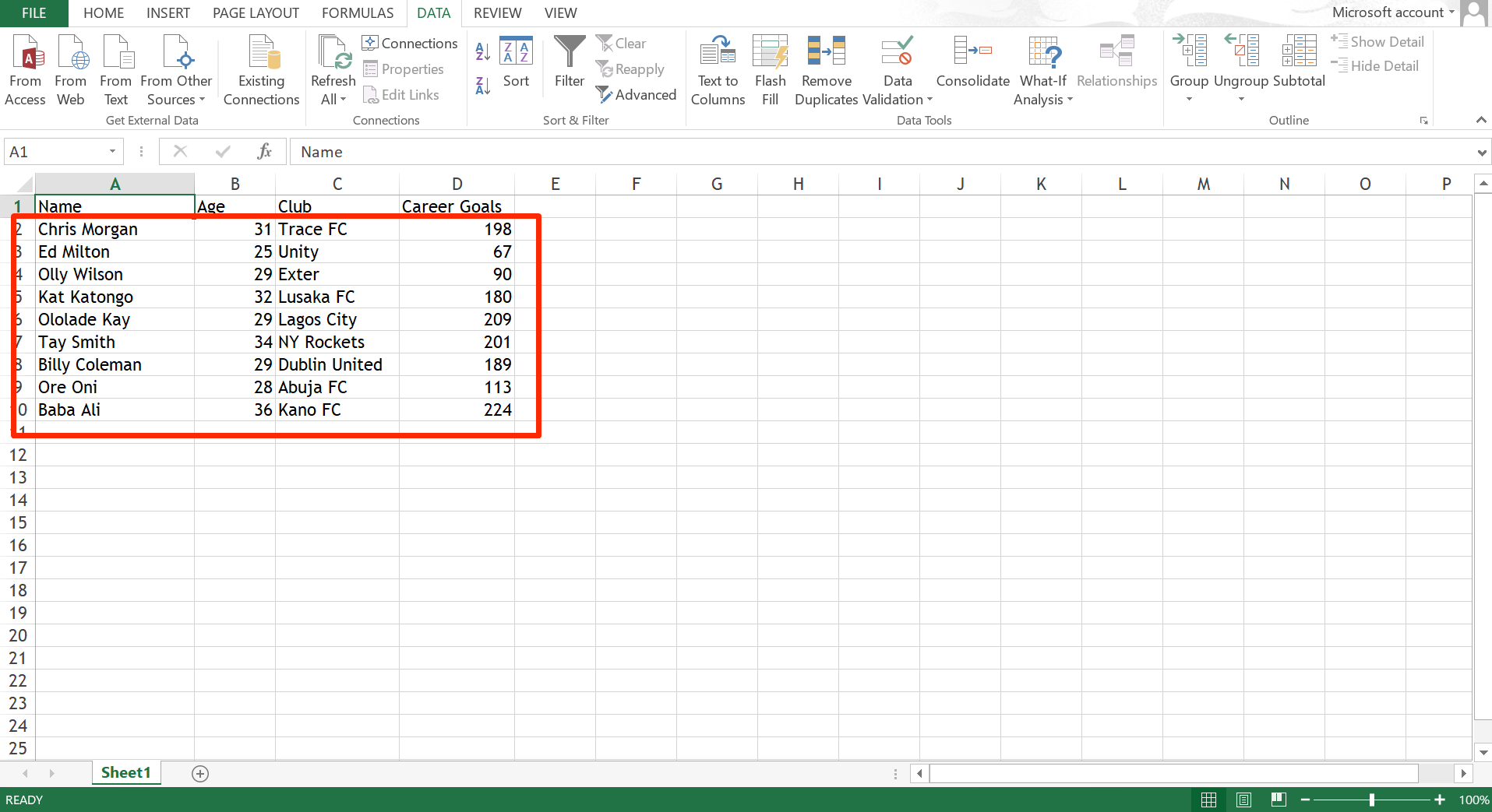
1. Open your Excel spreadsheet and select any range in your spreadsheet which you want to delete duplicate rows from.

How to Find and Remove Duplicates in Excel — Find duplicate rows

2. Go to Data > Remove duplicates.

How to Find and Remove Duplicates in Excel — Remove duplicates

If you haven’t selected all data in your spreadsheet, Excel will give you the option of expanding the search to the entire document, which is recommended. Click “OK”.

3. In case your data selection has headers, tick the column boxes that contain them so as not to be counted in the duplicate search. All columns in my example contain headers, so I’ll leave all boxes ticked. Click “OK”.

How to Find and Remove Duplicates in Excel — Remove headers from duplicate search

4. Excel prompts you with a dialog box informing you about the exact number of duplicate values it found and removed, as well as the number of unique values remaining in your spreadsheet.

How to Find and Remove Duplicates in Excel — Duplicate values found

How to Combine Multiple Excel Columns Into One?

There are many ways to combine multiple columns into a single column in Excel. Here’s how to do it without losing any data

How to delete duplicates in Excel but keep one?

Although the previous method is helpful at targeting all duplicates, this means that the unique data will also be permanently deleted. To avoid this, you may want to explore the following methods.

Here’s how to delete duplicates in Excel but keep one; we strongly recommend that you always keep a copy spreadsheet in case you want to go back to the original dataset.

How to remove duplicates using the Advanced Filter option?

This is a straightforward way to get rid of any duplicate content without deleting them entirely; instead, the Advanced filter option hides your duplicates from your dataset.

1. Select a cell in your dataset and go to Data > Advanced filter to the far right.

How to Find and Remove Duplicates in Excel — Advanced filter

2. Choose to “Filter the list, in-place” or “Copy to another location”. The first option will hide any row containing duplicates, while the second will make a copy of the data.

How to Find and Remove Duplicates in Excel — Filter list

Leave the “List range” field empty, if you want Excel to list it automatically. You can also leave the “Criteria range” empty. The only mandatory field to fill out is the “Copy to” if you selected the “Copy to another location” option.

3. Tick the “Unique records only” box to keep the unique values, and then “OK” to remove all duplicates.

How to Find and Remove Duplicates in Excel — How to keep unique values

Advanced filters are an excellent way to remove duplicate values while keeping a copy of the original data. Don’t forget that the Advanced filter option only applies to the entire table.

How to remove duplicates using Excel formulae?

Although you can combine various formulae to remove duplicates in Excel, in 2018, Microsoft integrated the UNIQUE formula to make this process much easier. First, let’s explore the syntax of the UNIQUE formula:

=UNIQUE (array, [by_col], [exactly_once])

array refers to the range of cells we will extract unique values from and represents the only required argument.
[by_col] is an optional parameter determining the search for unique values by rows or columns.
[exactly_once] is the other optional parameter and sets the behavior for values that appear more than once. If you want the formula to return items that appear exactly once, then write “TRUE”; however, if you want it to return every distinct item, then write “FALSE”.

Let’s now apply the =UNIQUE formula to our dataset.

1. Enter the formula next to the set of data. You can either leave one column in between or place it directly next to the last data column. Like in most Excel formulae, as soon as you type at the beginning of the formula, the rest will prompt automatically. Select the range you want to apply the formula to.

How to Find and Remove Duplicates in Excel — UNIQUE formula

2. You can leave the second parameter [by_col] by simply including the comma before and after its place. Let’s first see what happens when we include “TRUE” for the [exactly_once] parameter.

How to Find and Remove Duplicates in Excel — UNIQUE function

3. As soon as you press the Return key, Excel removes all duplicates. In this example, it has removed rows 5 and 6.

How to Find and Remove Duplicates in Excel — TRUE UNIQUE formula

Let’s see how by including “FALSE” as the last parameter, Excel will keep the unique value.

1. Follow the previous steps, and now wrote “FALSE”, to return every distinct value.

How to Find and Remove Duplicates in Excel — FALSE UNIQUE formula

2. Now, the UNIQUE formula has returned row 5 and only deleted the duplicate value in row 6.

How to Find and Remove Duplicates in Excel — FALSE UNIQUE formula return

How to remove duplicates using conditional formatting?

Conditional formatting is an Excel feature that helps users filter, sort, and organize data according to built-in rules or custom ones created by the user. The most common feature is the “Highlight Cell Rules”, which allows you to format cell values according to color, font, and various other format styles. Although this method won’t directly remove duplicates, it will make them extremely clear to identify.

1. Select the range of cells you want to apply the conditional formatting rule to. Then go to Home > Conditional Formatting > Highlight Cell Rules > Duplicate Values.

How to Find and Remove Duplicates in Excel — Conditional formatting

2. Set the “Style” to “Classic” and then “Format only unique or duplicate values”. Don’t forget to leave the drop-down menu to “duplicate”. Finally, choose the formatting style using the “Format with” drop-down menu. Click “OK”.

How to Find and Remove Duplicates in Excel — Conditional formatting remove duplicates

3. You can see how Excel highlights all duplicate values, including the cells. This means that you will need to make sure to only remove rows unless you are actually interested in removing all duplicates.

How to Find and Remove Duplicates in Excel — Highlight duplicates conditional formatting]

In case you want to highlight rows, you can combine all row values in one cell using the =CONCAT formula; if you would like to learn more about this function, read this article on the Microsoft support page.

How to remove duplicates based on one or more columns in Excel?

As a more advanced use of Excel, you can remove duplicates based on one or more columns using Power Query. This feature allows you to select the columns you would like to remove the duplicates from. Let’s explore how to use Power Query to remove duplicates based on one or more columns.

1. Go to Data > Get Data (Power Query).

How to Find and Remove Duplicates in Excel — Power Query

2. Choose “Excel workbook” as your data source.

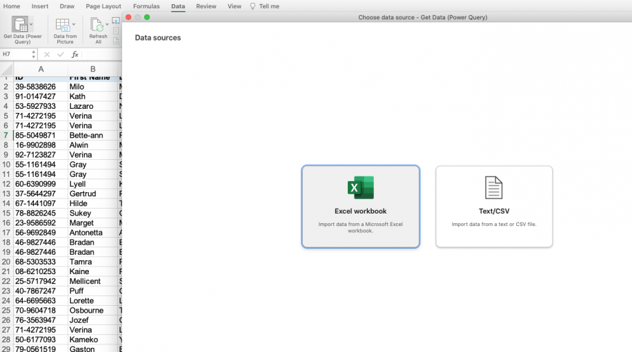
How to Find and Remove Duplicates in Excel — Power Query data source

3. Browse through your files and select the spreadsheet you want to apply the Power Query function to. Click “Next”.

How to Find and Remove Duplicates in Excel — Power Query load data

4. Tick the checkbox next to the worksheet containing your data (located in the left-side menu). Then, click “Load” in the bottom right-hand corner.

How to Find and Remove Duplicates in Excel — Power Query load data

5. As you can see, the dataset has been transformed into a table.

How to Find and Remove Duplicates in Excel — Power Query table

6. Select the columns to apply the Power Query to by pressing Ctrl/Cmd + click on the columns.

How to Find and Remove Duplicates in Excel — Power Query table

7. To delete duplicates, simply click on “Remove Duplicates” in the “Data” tab. Then click “OK” in the pop-up dialog box.

How to Find and Remove Duplicates in Excel — Remove Duplicates

8. Excel will inform you about the number of duplicates removed and how many unique values remain.

How to Find and Remove Duplicates in Excel — Final Alert message

Don’t worry about removing all duplicates, since the dataset you worked on is a copy created by the Power Query function. However, if you want to keep unique values, follow the steps outlined in the sections on the Advanced Filter option or =UNIQUE formula in Excel.

Want to Boost Your Team’s Productivity and Efficiency?

Transform the way your team collaborates with Confluence, a remote-friendly workspace designed to bring knowledge and collaboration together. Say goodbye to scattered information and disjointed communication, and embrace a platform that empowers your team to accomplish more, together.

Key Features and Benefits:

Centralized Knowledge: Access your team’s collective wisdom with ease.
Collaborative Workspace: Foster engagement with flexible project tools.
Seamless Communication: Connect your entire organization effortlessly.
Preserve Ideas: Capture insights without losing them in chats or notifications.
Comprehensive Platform: Manage all content in one organized location.
Open Teamwork: Empower employees to contribute, share, and grow.
Superior Integrations: Sync with tools like Slack, Jira, Trello, and more.

Limited-Time Offer: Sign up for Confluence today and claim your forever-free plan, revolutionizing your team’s collaboration experience.

Conclusion

As we have seen, there are many ways to identify and eliminate duplicates in your data, depending on your needs. Not only can you now successfully organize your data correctly, but removing duplicates makes it easier to identify key patterns and create accurate reports, particularly when working with larger datasets.

Источник

What is the Remove Duplicates in Excel Feature?

Remove Duplicates is an Excel feature that searches for repeated data in the selected cell range and performs the delete operation to provide a data set with unique values.

For example, the image below illustrates a table with multiple entries for James and Alan. When we use the Remove Duplicates feature in Excel, we get the table with unique values.

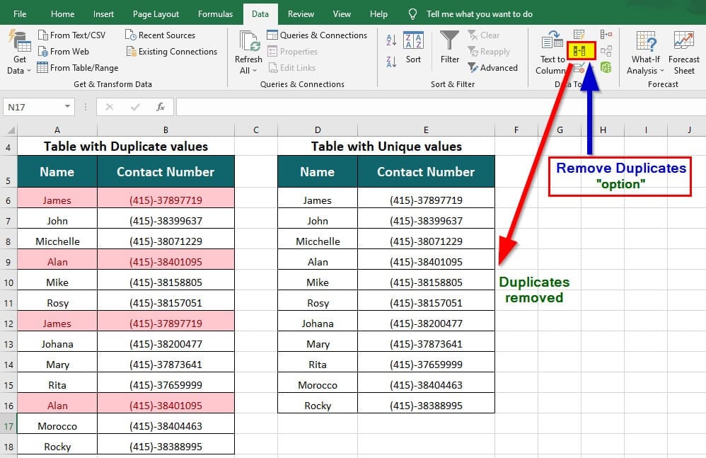
This feature can remove duplicates from a large accounting database while preparing sales reports or any data with repeated entries.

Key Highlights

We can use conditional formatting to highlight duplicate values.
To remove duplicates, we must filter the highlighted values and manually delete them.
The Remove Duplicates in Excel feature permanently deletes (removes) duplicate values from a worksheet.
Excel cannot find and remove duplicates from the area section of a Pivot Table report

How to Remove Duplicates in Excel?

You can download this Remove Duplicates in Excel here – Remove Duplicates in Excel

#1 Using Conditional Formatting

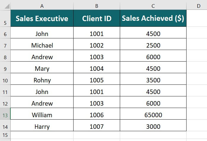
The table below shows the names of Sales executives, along with their Client IDs and sales. We want to find any duplicate values in the data using conditional formatting.

Solution:
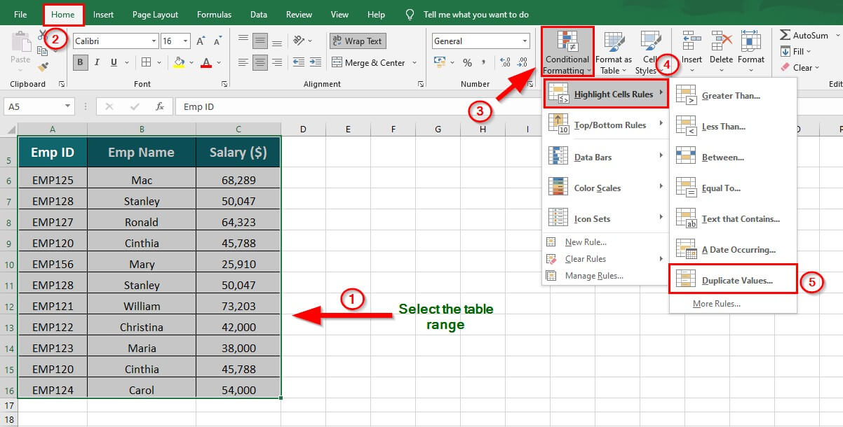
Step 1: Select the data table
Step 2: Go to the Home Tab
Step 3: Go to Conditional formatting > Highlight Cells Rules > Duplicate Values

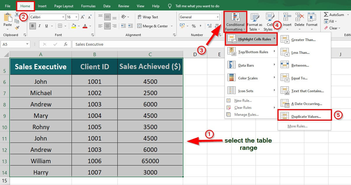
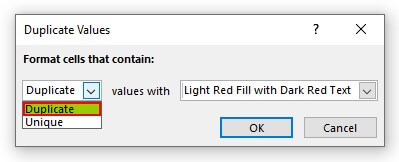
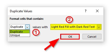
A Duplicate values dialog box will appear
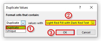
Step 4: Select Duplicate from the drop-down list as shown below

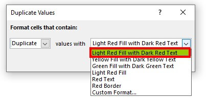
Step 5: Choose the desired highlight color

Step 6: Click on OK

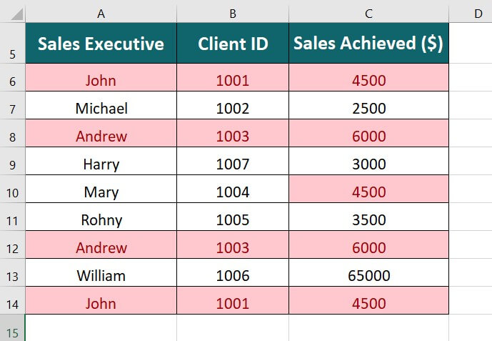
The duplicate values are highlighted as shown below

#2 Using the Filter Option to Remove Duplicates in Excel

The below table shows highlighted duplicate values. To remove the duplicate rows follow the given steps.

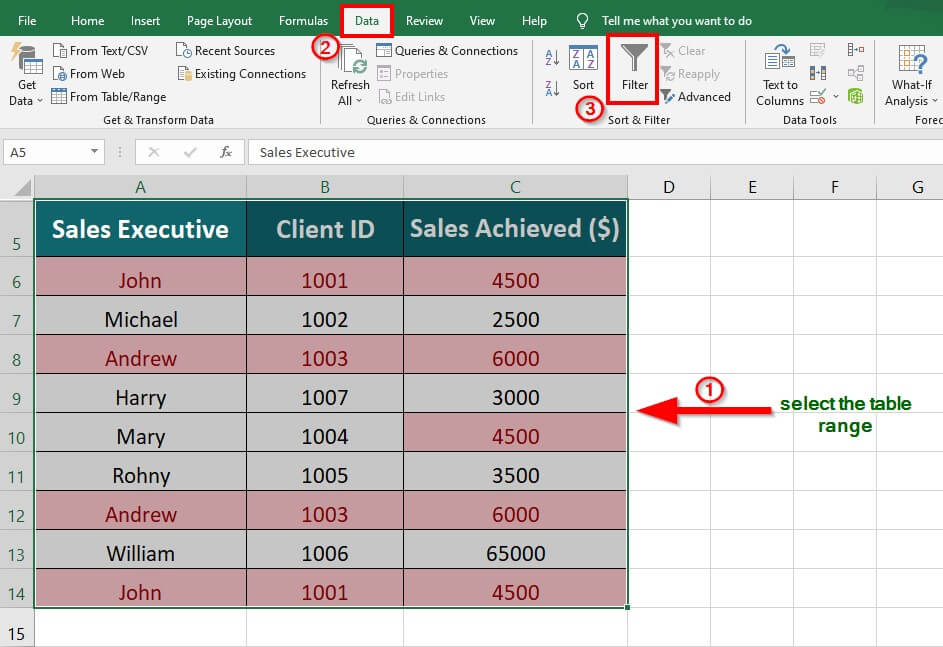
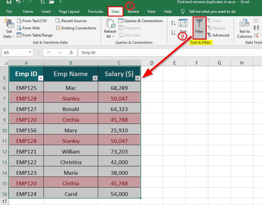
Step 1: Select the data table
Step 2: Go to Data Tab
Step 3: Under the Sort & Filter Group select the Filter option

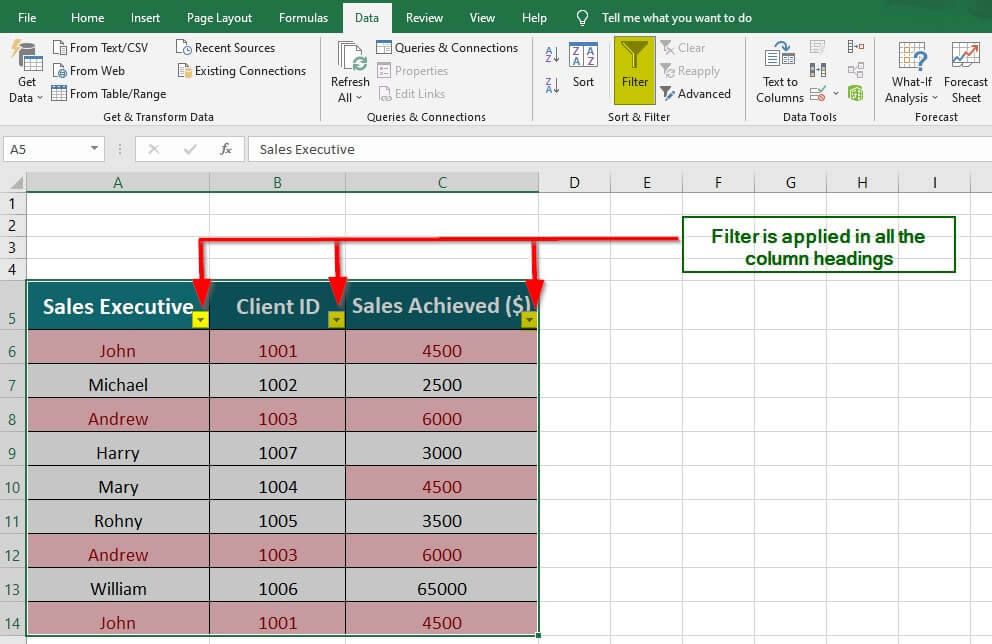
A filter is applied to all the columns

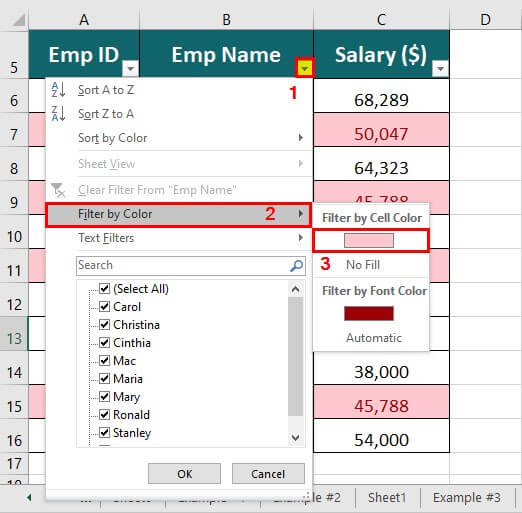
Step 4: Click the filter icon of column B (Client ID)
Step 5: Click on Filter by Color
Step 6: Select Filter by Cell Color

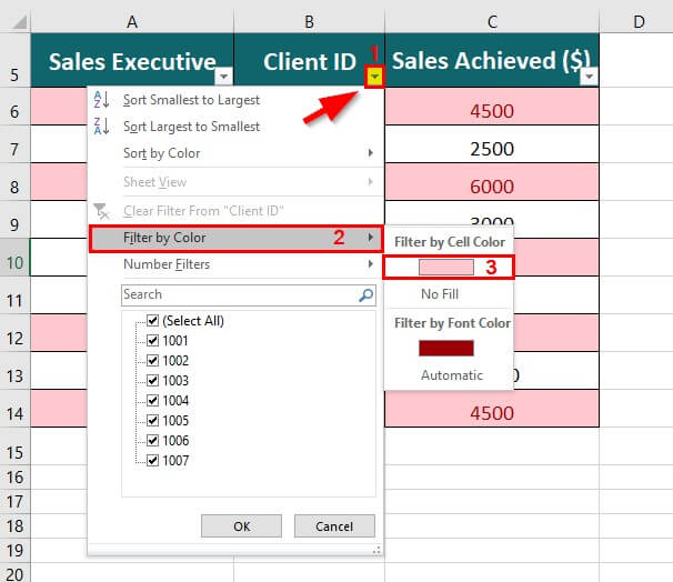
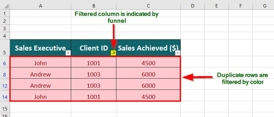
The highlighted (duplicate) rows are filtered as shown below

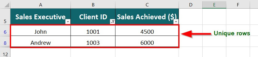
Step 7: Delete the duplicate rows manually to get Unique values

Shortcut: To apply a filter, select the desired table range and press the keys CTRL + SHIFT + L together.

#3 Using the Remove Duplicates Feature in Excel

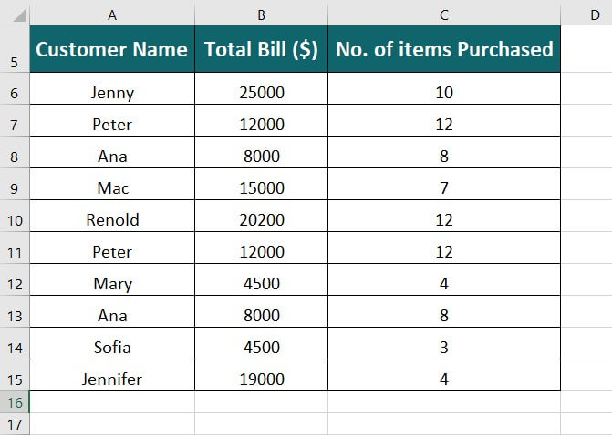
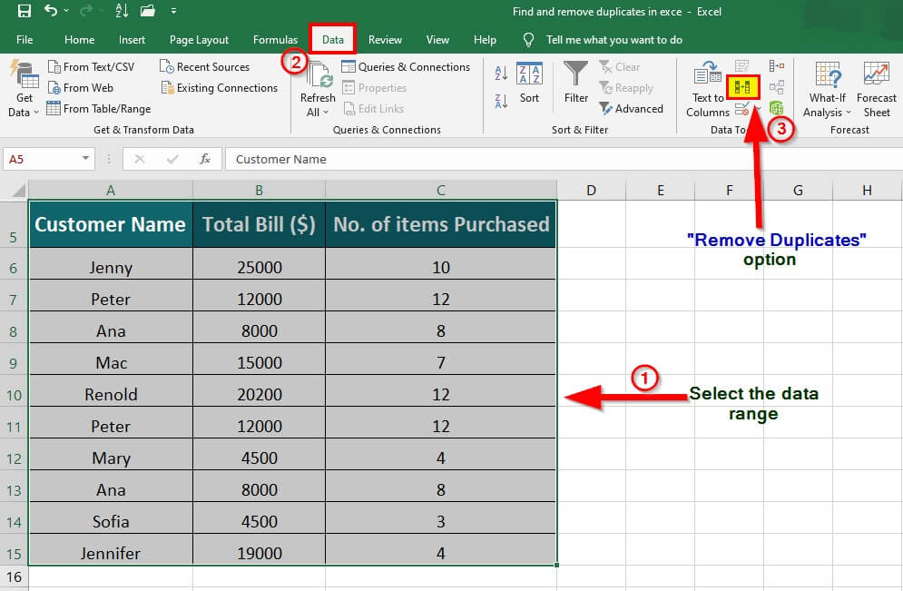
The table below displays a list of customers along with their Total Bill and the number of items purchased. We want to remove duplicate entries from the list using the Remove Duplicates feature.

Solution:
Step 1: Select the data table
Step 2: Go to Data Tab
Step 3: Click the Remove Duplicates icon under the Data Tools Tab.

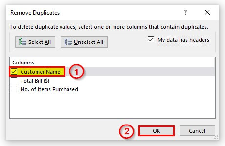
A Remove Duplicates dialog box appears
Step 4: Select the column headings (customer Name) by which the duplicate value needs to be searched
Step 5: Click OK

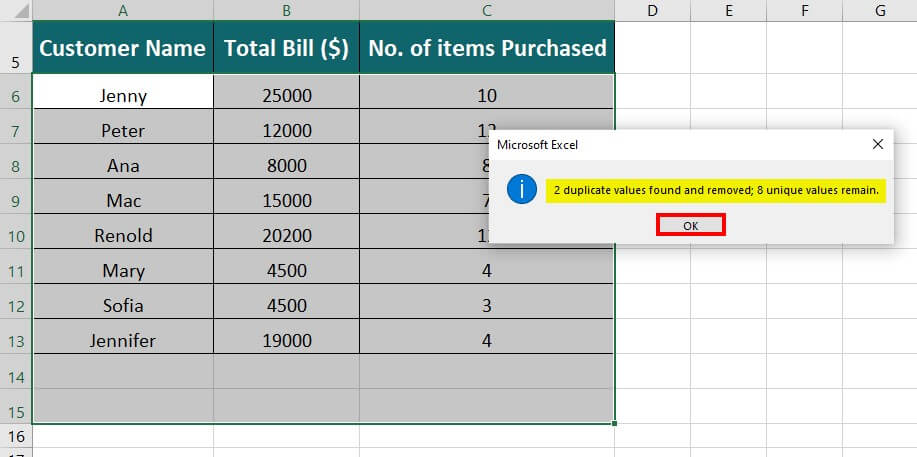
A Microsoft Excel pop-up indicates the number of duplicate values found and removed; and the number of unique values that remain.
Step 6: Click OK

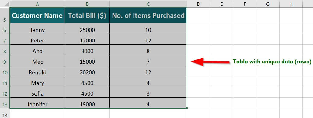
All the duplicate values are removed and the table now consists of unique values.

#4 Using the COUNTIF Function to Find the Number of Duplicates

We can find the number of duplicate values in a given data set using the COUNTIF function in Excel. Consider the following example to understand how it works.

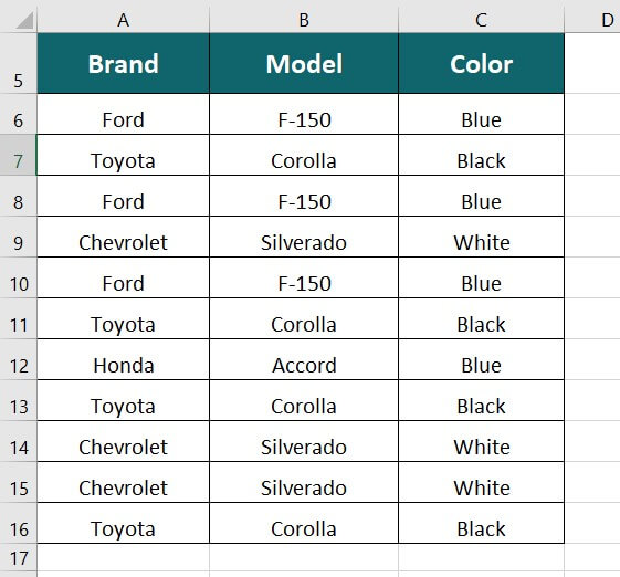
The table below shows the Brand names of four-wheelers with the Model name and colors. We want to find the number of duplicate values using the COUNTIF function in Excel.

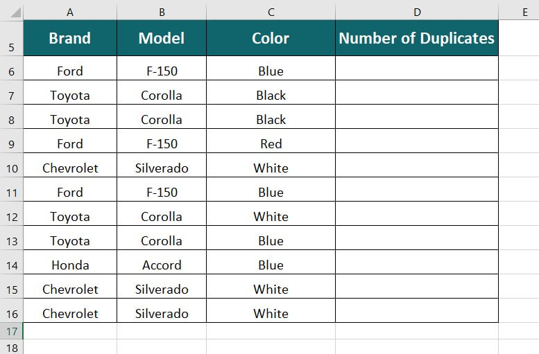
Solution:
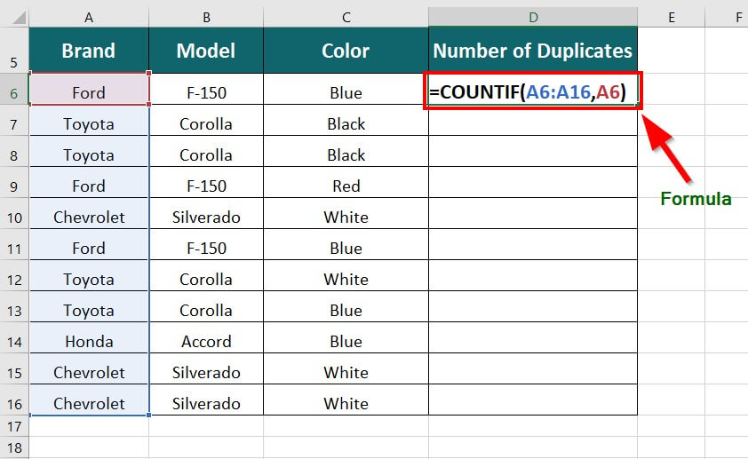
Step1: Place the cursor in cell D6 and enter the formula,

=COUNTIF(A6:A16,A6)

A6:A16 – It is the range across which we want to find the duplicate data
A6 – It indicates the first value in the range A6:A16

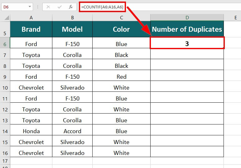
Step 2: Press Enter key to get the total number of duplicates (3) for the brand Ford.

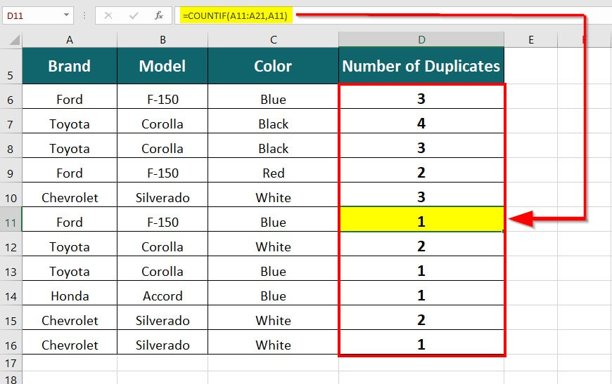
Step 3: Drag the formula in the remaining cells to get the number of duplicates as shown below

#5 Using Advanced Filter to Remove Duplicates in Excel

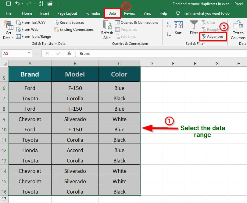
The table below shows the brand name of four-wheelers, as well as their model name and color. Using Excel’s Advanced Filter, we want to remove the duplicate values.

Solution:
Step 1: Select the data range
Step 2: Go to Data Tab
Step 3: Select the Advanced option under the Sort & Filter Group.

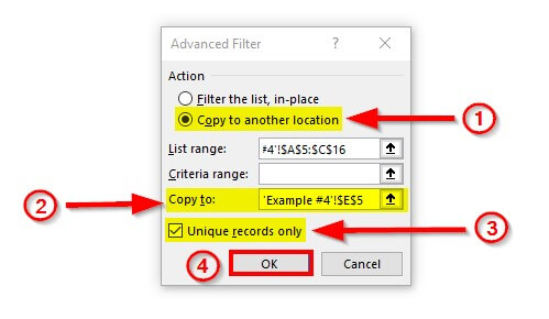
An Advanced Filter dialog box appears
Step 4: Select the Copy to another location option
Step 5: Click the cell in the worksheet where the new(unique) data table needs to be created. This will fill the section Copy to.
Step 6: Click the checkbox Unique records only.

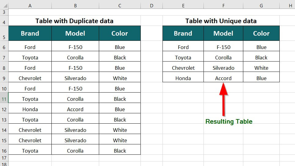
This results in a table with unique data, as shown below

#6 Using the Power Query Tool in Excel to Remove Duplicates

You can integrate data from different sources, clean up your data, and transform it using Excel’s Power Query feature. Duplicates in Excel can be easily removed using this utility.

Step 1: Choose a cell or region, then find the Data Tab’s – Get & Transform Data section and click on the From Table/Range option.

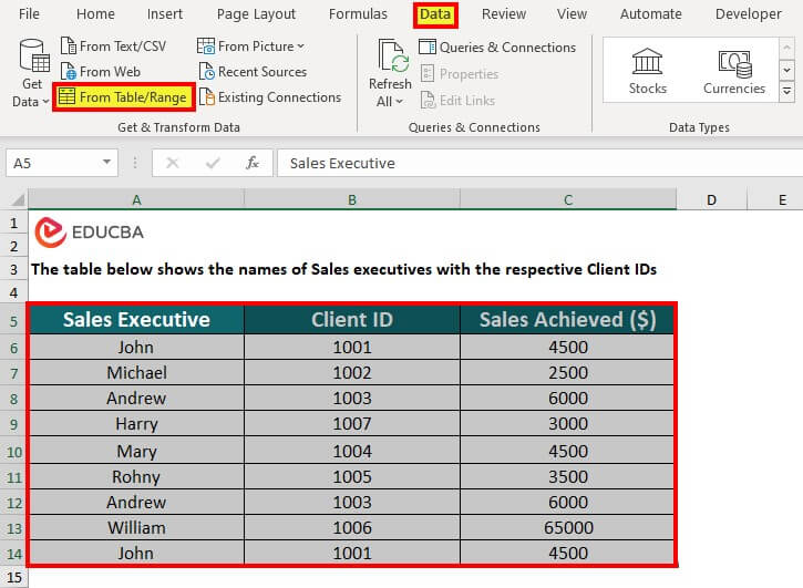
A dialogue window for creating a power query table will appear on clicking.
Step 2: Verify that the stated range of values is accurate.

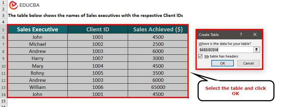
Step 3: Select OK.
The Power Query editor window opens.

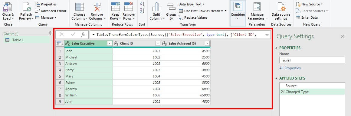
We now have two choices. Based on the following, copies can be eliminated:

One or more columns
Entire table

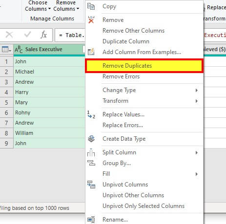
Step 4: Right-click on the relevant ‘column heading’ to delete duplicate entries based on one or more columns. Using the SHIFT button, we can pick multiple columns. In this example we have selected the Sales Executive column.

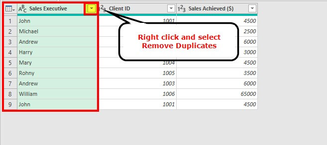
Step 5: Select the “Remove Duplicates” choice after that.

The data will be free of duplicate values in this manner.

Step 6: Clicking the “Close & Load” choice in the upper left corner will load the data onto the spreadsheet.

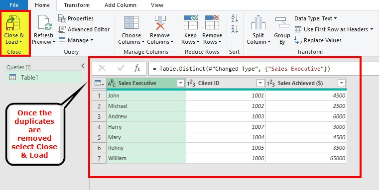
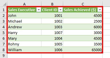
The data will be visible as per the below screenshot.

Things to Remember

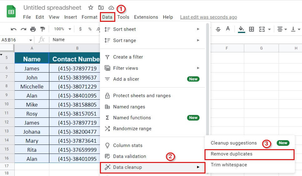
We can remove duplicates from Google Sheets using the Data Cleanup option
It is important to remove any subtotal before using the feature Remove Duplicates in Excel.
It is recommended to make a copy of your worksheet before trying to remove duplicate data.

Frequently Asked Questions (FAQs)

Q1. How do I quickly delete duplicates in Google Sheets?

Answer: To delete duplicates in Google Sheets, follow these steps:
Step 1: Select the data table
Step 2: Go To Data > Data cleanup > Remove duplicates

FAQ 1

Q2. Where is remove duplicates in Excel?

Answer: To find the Remove Duplicates option in Excel, follow these steps:
Step 1: Go to the Data Tab of the Excel toolbar
Step 2: Under the Data Tools Group click on the Remove Duplicates icon (option), as shown below

FAQ 2

Q3. What is the shortcut to find duplicates in Excel?

Answer: To find and highlight duplicates in Excel, press the below keys one by one,

ALT + H + L + H + D.

When we press the above keys, the duplicate values (rows) will be highlighted in the provided color. The keys function as a shortcut for the conditional formatting features in Excel.

Q4. How do I find and keep only duplicates in Excel?

Answer: To find and keep the duplicate values in Excel, follow the below steps:
Step 1: Select the data table
Step 2: Go to the Home Tab
Step 3: Under the Styles Group, go to,

Conditional Formatting > Highlight Cells Rules > Duplicate Values

FAQ 4

A Duplicate Values dialog box will appear,

Step 4: Select the Duplicate option from the drop-down list and choose the desired highlight color and Click OK

Step 4

All the duplicate values in the table will be highlighted.

Step 5: Select the data table and go to Data Tab
Step 6: Under the Sort & Filter Group click on Filter

This will apply a filter to the data set, as shown below

step 6

Step 7: Click on the filter icon of column B (Emp Name)
Step 8: Click on Filter by Color
Step 9: Select Filter by Cell Color

step 9

The highlighted duplicate values will be filtered as shown below

9.1

How to Find and Remove Duplicates with Conditional Formatting

If you need to selectively remove some duplicates (but leave others), this is the method to use. Here’s how it works:

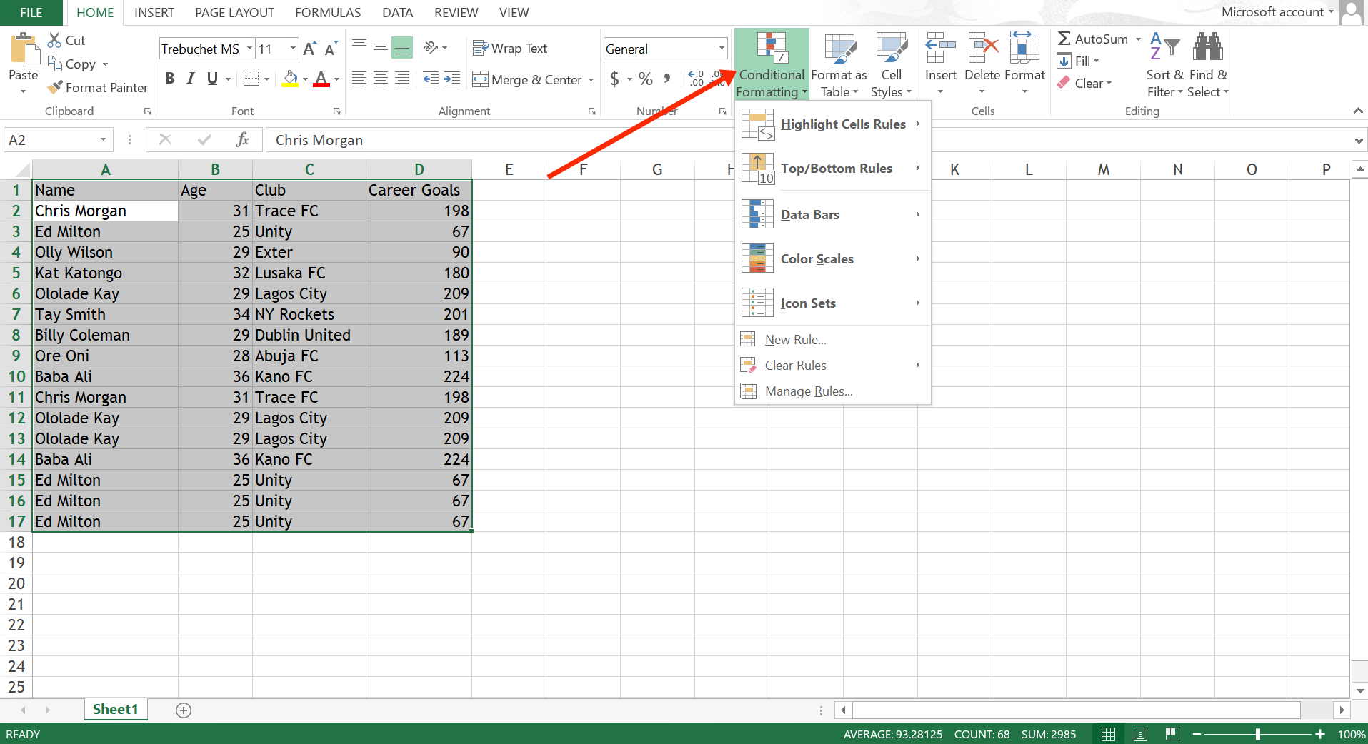
Step 1: Press CTRL + A to highlight the entire table, switch to the Home tab, then click on “Conditional Formatting”.
ss1

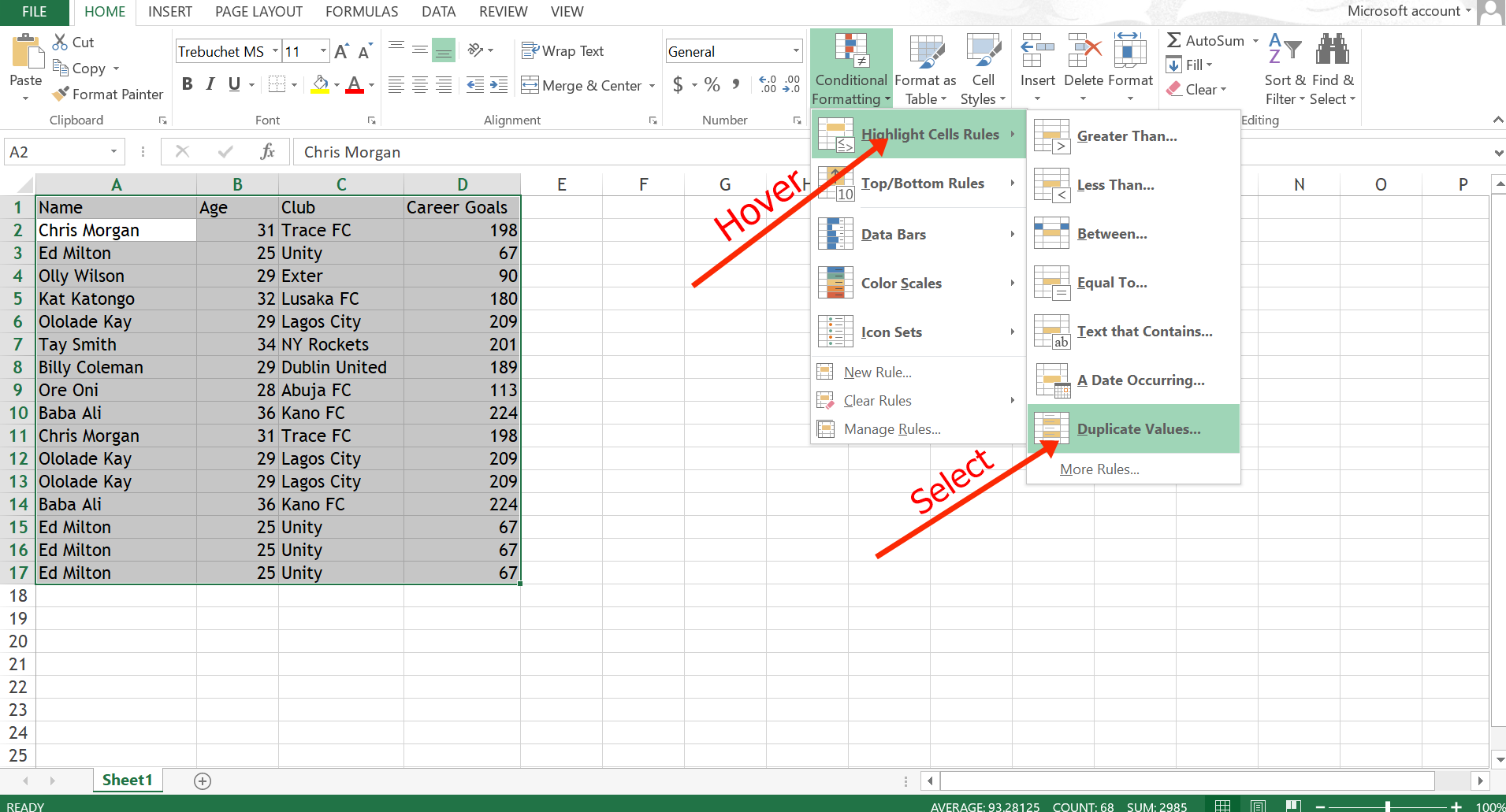
Step 2: Hover over “Highlight Cell Rules” and select “Duplicate Values”.
ss2

Step 3: Select how you want the duplicates to be highlighted, then click “Ok”.
ss3

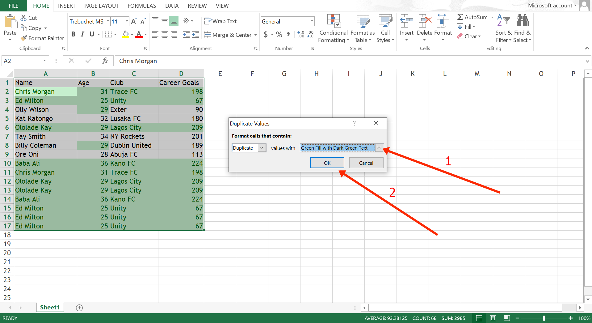
Duplicate cells will now be highlighted for you so you can remove the ones you don’t need:
ss4

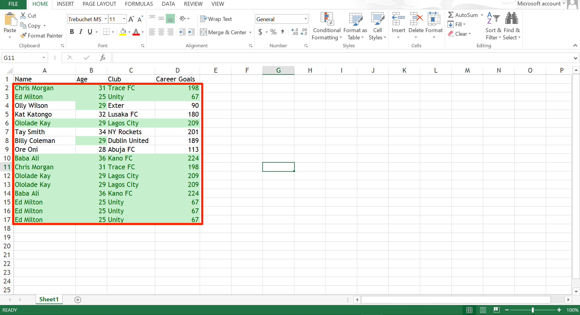
Again, on some occasions, you will need some duplicate entries. This method does not remove the duplicates automatically so you can do it yourself.

The next method removes duplicates automatically.

How to Remove Duplicates with the Remove Duplicate Command

This is one of the most reliable and straightforward ways to remove duplicates.

To use this method, follow the steps below:
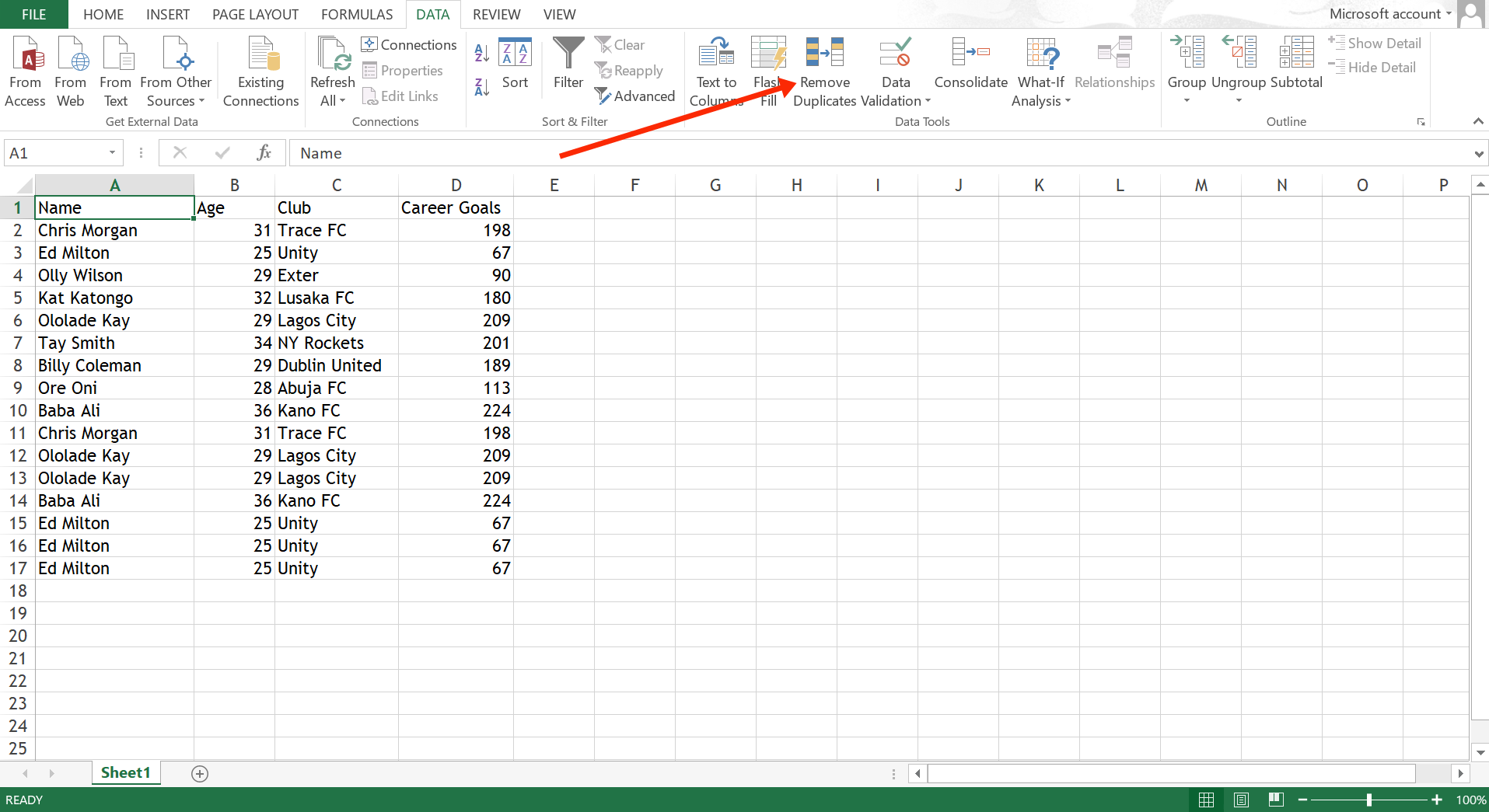
Step 1: Switch to the Data tab and click on “Remove Duplicates”.
ss5

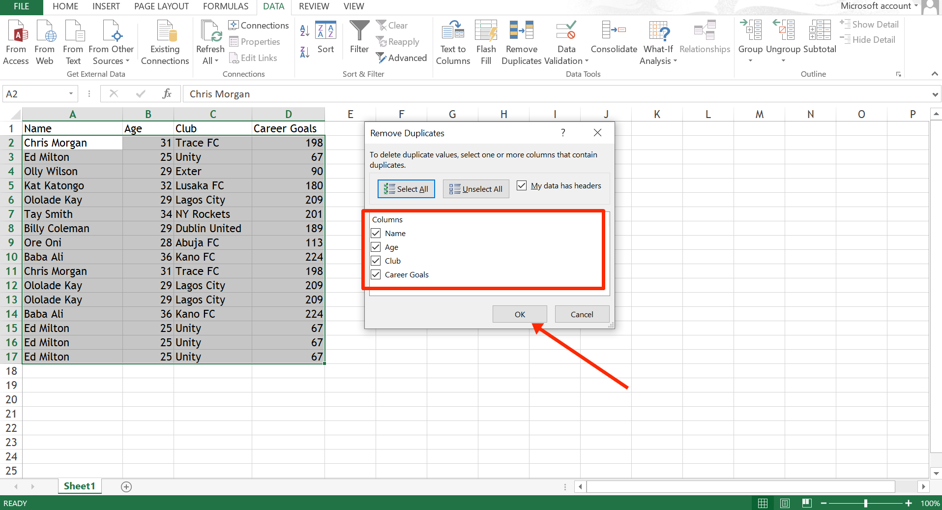
Step 2: Select all the columns in the table so Excel can look through and check for duplicates, then click “Ok”.
ss6

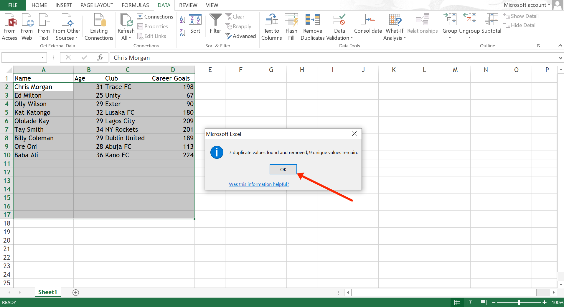
Step 3: You will get a message that duplicates have been removed. Click “Ok” to get rid of the message.
ss7
ss8

Conclusion

Duplicates can be a bottleneck for your productivity in Excel. Now that you know how to remove duplicates you can keep working effectively.

If this article helped you out, consider sharing it with your friends and family.

Thank you for reading.

Learn to code for free. freeCodeCamp’s open source curriculum has helped more than 40,000 people get jobs as developers. Get started

Источник

Remove duplicate values

Need more help?

Need more help?

Video Tutorial

What Is A Duplicate Value?

Find And Remove Duplicate Values With The Remove Duplicates Command

Find And Remove Duplicate Values With Advanced Filters

Find And Remove Duplicate Values With A Pivot Table

Find And Remove Duplicate Values With Power Query

Remove Duplicates Based On One Or More Columns

Remove Duplicates Based On The Entire Table

Keep Duplicates Based On A Single Column Or On The Entire Table

Find And Remove Duplicate Values Using A Formula

Find And Remove Duplicate Values With Conditional Formatting

Find And Remove Duplicate Values Using VBA

Conclusions

About the Author

CONTENTS:

Find and Highlight Duplicates in Excel

Finding and Highlight Duplicates in a Single Column in Excel

Finding and Highlight Duplicates in Multiple Columns in Excel

Finding and Highlighting Duplicate Rows in Excel

Remove Duplicates in Excel

Remove Duplicates from a Single Column in Excel

Remove Duplicates from Multiple Columns in Excel

Remove Duplicate Rows in Excel

How to find and remove duplicate rows in Excel?

How to Check for Duplicates in Excel?

How to remove duplicates using the Remove Duplicates feature?

How to Combine Multiple Excel Columns Into One?

How to delete duplicates in Excel but keep one?

How to remove duplicates using the Advanced Filter option?

How to remove duplicates using Excel formulae?

How to remove duplicates using conditional formatting?

How to remove duplicates based on one or more columns in Excel?

Want to Boost Your Team’s Productivity and Efficiency?

Conclusion

What is the Remove Duplicates in Excel Feature?

Key Highlights

How to Remove Duplicates in Excel?

#1 Using Conditional Formatting

#2 Using the Filter Option to Remove Duplicates in Excel

#3 Using the Remove Duplicates Feature in Excel

#4 Using the COUNTIF Function to Find the Number of Duplicates

#5 Using Advanced Filter to Remove Duplicates in Excel

#6 Using the Power Query Tool in Excel to Remove Duplicates

Things to Remember

Frequently Asked Questions (FAQs)

Q1. How do I quickly delete duplicates in Google Sheets?

Q2. Where is remove duplicates in Excel?

Q3. What is the shortcut to find duplicates in Excel?

Q4. How do I find and keep only duplicates in Excel?

Recommended Articles

How to Find and Remove Duplicates with Conditional Formatting

How to Remove Duplicates with the Remove Duplicate Command

Conclusion