
A big part of processing data involves the cleaning of the data.
Most data you bring in to Excel often comes from various sources. Many times they are converted from a different format. As such, it is not uncommon to find unwanted characters inside text string data.
What’s more annoying is that sometimes these unwanted characters are invisible. So they fail to give expected results when operations are performed on them. Another common problem is the presence of inconsistent blank spaces.
In this tutorial, we will address all the above issues using Excel functions, formulas, and features. We will see how to use various Excel functionalities to remove specific characters from strings in your cells.
Removing a Specific Character with the Find and Replace Feature
Excel’s Find and Replace dialog box is a great way to find items on your worksheet and get things done quickly.
All you need to do is enter your search string to specify what you want to replace and then specify what you want to replace it with.
Suppose you have the below dataset and you want to remove all the ‘@’ characters from the text string in each cell.

Below are the steps to remove a specific character using Find and Replace:
- Select the range of cells you want to work with.
- Click on Find & Select from the Home tab (under the ‘Editing’ group).

- This will display a dropdown menu. Select ‘Replace’.
- This will open the Find and Replace dialog box. Type ‘@’ in the text box next to ‘Find what’.
- Leave the text box next to ‘Replace with’ blank. This is because you want to remove any instance of the ‘@’ symbol in each cell.
- Click on the ‘Replace All’ button.


This will remove all instances of the ‘@’ symbol from all the cells.

Removing a Specific Character with the SUBSTITUTE Function
The SUBSTITUTE function can be used to remove a specific character from a string or replace it with something else. The general syntax for this function is:
=SUBSTITUTE (original_string, old_character, new_character, instance_number)
Here,
- original_string is the text or reference to the cell that you want to work on.
- old_character is the character that you want to replace.
- new_character is the character that you want to replace old_character with.
- instance_number is optional. It is the instance of the old_character that you want to replace.
It is possible to customize the above formula to the make it suitable to remove a specific character from a string, as follows:
=SUBSTITUTE (original_string, old_character, “”)
This formula will replace the old_character with a blank (“”), which means the character will basically get deleted.
Let us assume you have the same set of string values with the ‘@’ symbol in random places, and you want to remove all of them:
For this, you can use the SUBSTITUTE function with the following steps:
- Select the first cell of the column where you want the results to appear. In our example, it will be cell B2.
- Type the formula:
=SUBSTITUTE(A2,"@","")
- Press the return key.
- This will give you the text obtained after removing all instances of the ‘@’ symbol in cell A2.

- Double click the fill handle (located at the bottom-left corner) of cell B2. This will copy the formula to all the other cells of column B. You can also choose to drag down the fill handle to achieve the same effect. Here are both the original and converted columns side by side:

- If you want to retain only the converted versions of the text, then select these cells (B2:B5), copy them, and paste them in the same place as values.
- You can then delete column A if you need to.


Also Read: How to Remove the Last Digit in Excel?
Removing only a Particular Instance of a Specific Character in a String
Now, what if you wanted to remove just the first ‘@’ symbol from each cell, instead of all instances of them?
This is where the last optional parameter of the SUBSTITUTE function comes in handy.
Using this, you can specify which instance of the symbol you want to remove. So, to remove the first instance of a symbol, your function should be:
SUBSTITUTE (original_string, old_character, “”,1)
Similarly, if you want to remove the second instance of the character, the function will be:
SUBSTITUTE (original_string, old_character, “”,2)
Let’s see the steps to remove only the first instance of the ‘@’ symbol from the above dataset:
- Select the first cell of the column where you want the results to appear. In our example, it will be cell B2.
- Type the formula:
=SUBSTITUTE(A2,"@","",1)
- Press the return key.
- This will give you the text obtained after removing only the first ‘@’ symbol in cell A2.

- Double click the fill handle (located at the bottom-left corner) of cell B2. This will copy the formula to all the other cells of column B. You can also choose to drag down the fill handle to achieve the same effect. Here are both the original and converted columns side by side:

- If you want to retain only the converted versions of the text, then select these cells (B2:B5), copy them, and paste them in the same place as values.
- You can then delete column A if you need to.


Also read: How to Remove First Character in Excel?
Removing any Special Character with the CLEAN Function
The Excel CLEAN function removes line breaks and non-printable characters from a string. The general syntax for this function is:
=CLEAN (original_string)
Here, original_string is the text or reference to the text cell that you want to clean.
The result is the text that has all non-printable characters removed.
Let’s take a look at the following set of strings.

Since the list was brought in from another application, it ended up having a lot of unnecessary characters, like new-line characters, spaces, etc.
Let’s see how to use the CLEAN function to clean this data:
- Select the first cell of the column where you want the results to appear. In our example, it will be cell B2.
- Type the formula:
=CLEAN(A2).
- Press the return key.
- This will give you the text obtained after removing all line breaks from the string in cell A2.
- Double click the fill handle (located at the bottom-left corner) of cell B2. This will copy the formula to all the other cells of column B.

Notice that the new line characters got removed, but the results still don’t look right. This is because when the data was brought in, it also contained some space characters, besides the new lines.
The CLEAN function removes only the first 32 (non-printable) characters in the 7-bit ASCII code (i.e. values 0 to 31). However, there are other non-printable characters in Unicode that CLEAN cannot remove.
Since the space character has a value of 32, the CLEAN function does not remove spaces. So it is best to apply the TRIM function after applying the CLEAN function to remove the spaces.
Removing Leading or Trailing Space Characters with the TRIM Function
A lot of data cleaning merely consists of removing leading or trailing space characters from strings. Excel’s TRIM function makes this easy to do in just one go.
The TRIM function removes the space character (“ “) from the text. If the spaces are leading or trailing spaces, it removes all of them. If there are extra spaces between words, then it removes the extras and leaves just a single space.
The general syntax for this function is:
=TRIM (original_string)
Here, original_string is the text or reference to the text cell that you want to process.
Let us use the TRIM function to remove the space characters that were left over after applying the CLEAN function:

- Select the first cell of the column where you want the results to appear. In our example, it will be cell C2.
- Type the formula:
=TRIM(B2).
- Press the return key.
- This will give you the text obtained after removing all unnecessary spaces from the string in cell B2.
- Double click the fill handle (located at the bottom-left corner) of cell C2. This will copy the formula to all the other cells of column C.

- If you want to retain only the converted versions of the text, then select these cells (C2:C5), copy them, and paste them in the same place as values.
- You can then delete columns A and B if you need to.


Removing a Specific Invisible Character from a String using SUBSTITUTE, CHAR and CODE Functions
In some cases, both CLEAN and TRIM functions fail to remove some particularly annoying characters from the string.
This may be because these characters are neither spaces nor one of the 32 characters that the CLEAN function can remove.
You can find the code of a character by using the CODE function. For example, in the sample text below, there is an invisible character at the start of the string.
Since it couldn’t be removed with a TRIM or CLEAN, it is quite evident that it’s not a regular space.

Here’s what we can do to remove all instances of the invisible character:
- To find out what this character is, we can use the CODE function. Type this function into the cell B2: =CODE(LEFT(A2)). Since the character is in the first position in the text, we can easily find out its code using the LEFT function. In this case, we get the result as “160”. That means the invisible character’s code is 160.

- Let us use this value in the SUBSTITUTE function. Type this function into the cell C2: =SUBSTITUTE(A2,CHAR(B2),””). Here we used the CHAR function to convert the character code back to its character equivalent.
- When you press the return key now, you will find all instances of that invisible character removed from the string.


In this tutorial, we saw how you can use various Excel functions, formulas, and features to remove specific characters from a string.
If you know what the character you want to remove is, you can use either the Find and Replace feature or the SUBSTITUTE function.
To remove blank spaces and special characters (that often accompany data brought in from other applications) you can use the CLEAN and TRIM functions respectively.
If there are other invisible characters in the string and you don’t know what the characters are, you can use a formula that combines the CODE, CHAR, and SUBSTITUTE functions together.
We tried to put together all possible situations where you would need to remove a specific character from text in Excel.
Hope you found the tutorial useful!
Other Excel tutorials you may like:
- How to Remove Text after a Specific Character in Excel
- How to Remove Question Marks from Text in Excel?
- How to Remove Commas in Excel (from Numbers or Text String)
- How to Remove Dollar Sign in Excel
- How to Remove Apostrophe in Excel
- How to Add Text to the Beginning or End of all Cells in Excel
- How to Reverse a Text String in Excel (Using Formula & VBA)
- How to Change All Caps to Lowercase Except the First Letter in Excel?
- How to Extract Text After Space Character in Excel?
- Extract Last Name in Excel
- How to Separate Names in Excel
- How to Remove Space before Text in Excel
In this article, we will learn how to remove unwanted characters in Excel.
Sometimes you get uncleaned data set in excel & I don’t want you being banging your head on wall to clean the data set.
In simple words, Excel lets you clean unwanted characters using SUBSTITUTE function .
Syntax to clean unwanted characters
=SUBSTITUTE ( Text , «remove_char», «»)
“” : empty string
Let’s use this function on some of the uncleaned values shown below.
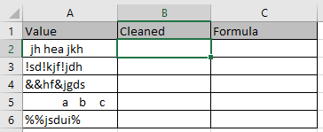
Let’s understand this one by one:
1st case:
When you need to remove just the spaces from the data set. Use the single space as remove_char in the formula
Formula
=SUBSTITUTE(A2,» «,»»)
Explanation:
This formula extracts every single space in the cell value and replaces it with an empty string.
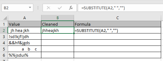
As you can see the first value is cleaned.
Second Case:
When you know a specific character to remove from the cell value, just use that character as remove_char in the formula
Use the formula
=SUBSTITUTE(A3,»!»,»»)
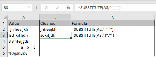
As you can see the value is cleaned.
Third Case:
When you wish to remove the character by using its code. This can help you in removing case sensitive character.
Just use the char(code) in place of remove_char. To know the code of the character uses the function shown below.

Use the formula to remove the character
=SUBSTITUTE(A4,CHAR(38),»»)

As you can see the value is cleaned.
Final Case:
When you wish to remove the character which comes at the first position in the text. You need to grab the code of the character using the LEFT & CODE function.
Use the formula
=SUBSTITUTE(A5,CHAR(CODE(LEFT(A5))),»»)
Explanation:
LEFT(A5) grabs the single space code in the formula using LEFT & CODE function and giving as input to char function to replace it with an empty string.
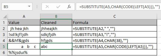

As you can see the value is cleaned in both the cases whether it is single space or any other character.
I hope you understood how to remove unwanted characters from the text using SUBSTITUTE function in Excel. Explore more articles on Excel TEXT function here. Please feel free to state your query or feedback for the above article.
Related Articles:
How to Remove leading and trailing spaces from text in Excel
How to use the RIGHT function in Excel
How to Remove unwanted characters in Excel
How to Extract Text From A String In Excel Using Excel’s LEFT And RIGHT Function
Popular Articles:
50 Excel Shortcuts to Increase Your Productivity
How to use the VLOOKUP Function in Excel
How to use the COUNTIF function in Excel
How to use the SUMIF Function in Excel
This post explains that how to remove unwanted characters from text string in a Cell in Excel. How do I remove unwanted characters from a cell using Excel formula.
Table of Contents
- Remove Unwanted Characters
- Related Formulas
- Related Functions
If you want to remove unwanted or specified characters from a text string, you can create an excel formula based on the SUBSTITUTE function and CHAR function.
You can use CHAR function get a character from a code number, then using SUBSTITUTE function to replace this character with empty string.
Assuming that you want to remove hash character from text string in Cell B1, then you can write down the following formula:
=SUBSTITUTE(B1,CHAR(35),"")
Let’s see how this formula works:
=CHAR(35)
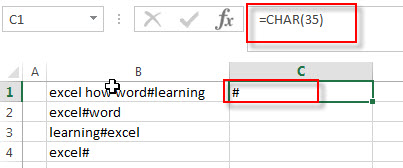
The CHAR function returns a character based on the given character code, and this function returns a hash character.
=SUBSTITUTE(B1,CHAR(35),” “)
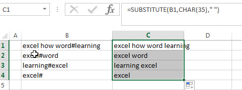
This formula will replace all hash character returned by the CHAR function with empty string, it means that it will remove all hash characters from text string in Cell B1.
You can refer to the below link for the character set:
Windows: http://en.wikipedia.org/wiki/Windows-1252
Mac: http://en.wikipedia.org/wiki/Mac_OS_Roman
- Remove all spaces between numbers or words
you want to remove all spaces between text character and numbers in those cells. You can use Excel Find & replace or SUBSTITUTE function. …. - Remove text before the first match of a specific character
If you want to remove all characters that before the first occurrence of the comma character, you can use a formula based on the RIGHT function, the LEN function and the FIND function….. - Extract text before first comma or space
If you want to extract text before the first comma or space character in cell B1, you can use a combination of the LEFT function and FIND function…. - Extract text after first comma or space
If you want to get substring after the first comma character from a text string in Cell B1, then you can create a formula based on the MID function and FIND function or SEARCH function …. - Extract text before the second or nth specific character
you can create a formula based on the LEFT function, the FIND function and the SUBSTITUTE function to Extract text before the second or nth specific character…
- Excel Substitute function
The Excel SUBSTITUTE function replaces a new text string for an old text string in a text string.The syntax of the SUBSTITUTE function is as below:= SUBSTITUTE (text, old_text, new_text,[instance_num])…. - Excel CHAR function
The Excel CHAR function returns the character specified by a number (ASCII Value). The syntax of the CHAR function is as below: =CHAR(number)….
Excel for Microsoft 365 Excel for Microsoft 365 for Mac Excel for the web Excel 2021 Excel 2021 for Mac Excel 2019 Excel 2019 for Mac Excel 2016 Excel 2016 for Mac Excel 2013 Excel 2010 Excel 2007 Excel for Mac 2011 Excel Starter 2010 More…Less
To get detailed information about a function, click its name in the first column.
Note: Version markers indicate the version of Excel a function was introduced. These functions aren’t available in earlier versions. For example, a version marker of 2013 indicates that this function is available in Excel 2013 and all later versions.
|
Function |
Description |
|---|---|
|
ARRAYTOTEXT function |
Returns an array of text values from any specified range |
|
ASC function |
Changes full-width (double-byte) English letters or katakana within a character string to half-width (single-byte) characters |
|
BAHTTEXT function |
Converts a number to text, using the ß (baht) currency format |
|
CHAR function |
Returns the character specified by the code number |
|
CLEAN function |
Removes all nonprintable characters from text |
|
CODE function |
Returns a numeric code for the first character in a text string |
|
CONCAT function |
Combines the text from multiple ranges and/or strings, but it doesn’t provide the delimiter or IgnoreEmpty arguments. |
|
CONCATENATE function |
Joins several text items into one text item |
|
DBCS function |
Changes half-width (single-byte) English letters or katakana within a character string to full-width (double-byte) characters |
|
DOLLAR function |
Converts a number to text, using the $ (dollar) currency format |
|
EXACT function |
Checks to see if two text values are identical |
|
FIND, FINDB functions |
Finds one text value within another (case-sensitive) |
|
FIXED function |
Formats a number as text with a fixed number of decimals |
|
LEFT, LEFTB functions |
Returns the leftmost characters from a text value |
|
LEN, LENB functions |
Returns the number of characters in a text string |
|
LOWER function |
Converts text to lowercase |
|
MID, MIDB functions |
Returns a specific number of characters from a text string starting at the position you specify |
|
NUMBERVALUE function |
Converts text to number in a locale-independent manner |
|
PHONETIC function |
Extracts the phonetic (furigana) characters from a text string |
|
PROPER function |
Capitalizes the first letter in each word of a text value |
|
REPLACE, REPLACEB functions |
Replaces characters within text |
|
REPT function |
Repeats text a given number of times |
|
RIGHT, RIGHTB functions |
Returns the rightmost characters from a text value |
|
SEARCH, SEARCHB functions |
Finds one text value within another (not case-sensitive) |
|
SUBSTITUTE function |
Substitutes new text for old text in a text string |
|
T function |
Converts its arguments to text |
|
TEXT function |
Formats a number and converts it to text |
|
TEXTAFTER function |
Returns text that occurs after given character or string |
|
TEXTBEFORE function |
Returns text that occurs before a given character or string |
|
TEXTJOIN function |
Combines the text from multiple ranges and/or strings |
|
TEXTSPLIT function |
Splits text strings by using column and row delimiters |
|
TRIM function |
Removes spaces from text |
|
UNICHAR function |
Returns the Unicode character that is references by the given numeric value |
|
UNICODE function |
Returns the number (code point) that corresponds to the first character of the text |
|
UPPER function |
Converts text to uppercase |
|
VALUE function |
Converts a text argument to a number |
|
VALUETOTEXT function |
Returns text from any specified value |


Important: The calculated results of formulas and some Excel worksheet functions may differ slightly between a Windows PC using x86 or x86-64 architecture and a Windows RT PC using ARM architecture. Learn more about the differences.
See Also
Excel functions (by category)
Excel functions (alphabetical)
Need more help?
Want more options?
Explore subscription benefits, browse training courses, learn how to secure your device, and more.
Communities help you ask and answer questions, give feedback, and hear from experts with rich knowledge.
Some text strings may include unwanted letters or extra characters that we don’t need. In order to remove letters from string, we will make use of the RIGHT or LEFT function, combined with the LEN function.
 Figure 1. Final result: Remove letters from string
Syntax of RIGHT, LEFT and LEN functions
RIGHT function returns the last characters in a text string,where num_chars is the number of characters
=RIGHT(text,[num_chars])
LEFT function returns the first characters in a text string,where num_chars is the number of characters
=LEFT(text,[num_chars])
LEN function – returns the number of characters in a text string
=LEN(text)
How to remove first character?
In order to delete the first character in a text string, we simply enter the formula using the RIGHT and LEN functions:
=RIGHT(B3,LEN(B3)-1)
 Figure 2. Output: Delete first character
The RIGHT function returns the last characters, counting from the right end of the text string. The number of characters is given by the LEN function.
LEN(B3)-1 means we remove 1 character from the value in B3 which is T6642. The resulting string minus the first character is 6642.
Remove first 3 characters
In order to remove three characters from a string, we still use the same formula but instead of 1, we subtract 3 characters. The formula becomes:
=RIGHT(B3,LEN(B3)-3)
The resulting text string is 42, as shown in C3 below.
 Figure 3. Output: Remove first 3 characters
How to remove last character?
In order to remove the last character, we will be using the LEFT and LEN functions:
=LEFT(B3,LEN(B3)-1)
 Figure 4. Output: Remove last character
The LEFT function returns the first characters, counting from the left end of the text string. The number of characters is given by the LEN function.
LEN(B3)-1 means we remove 1 character from the value in B3 which is T6642. The resulting string minus the last character is T664.
Instant Connection to an Expert through our Excelchat Service
Most of the time, the problem you will need to solve will be more complex than a simple application of a formula or function. If you want to save hours of research and frustration, try our live Excelchat service! Our Excel Experts are available 24/7 to answer any Excel question you may have. We guarantee a connection within 30 seconds and a customized solution within 20 minutes.
Formulas are key in getting things done in excel. One can apply formulas to manipulate texts, work with dates and time, count and sum with criteria, create dynamic ranges, and dynamically rank values. Explained below are formulas one can apply to remove characters in excel cells.
1. The Array Formula
Assuming we want to eliminate numbers from the following data

a) Select a bank cell you will return the text string without the letters.

Enter the formula;
=SUBSTITUTE(SUBSTITUTE(SUBSTITUTE(SUBSTITUTE(SUBSTITUTE(SUBSTITUTE(SUBSTITUTE(SUBSTITUTE(SUBSTITUTE(SUBSTITUTE(A1,1,»»),2,»»),3,»»),4,»»),5,»»),6,»»),7,»»),8,»»),9,»»),0,»»)
(A1 is the cell you will remove characters from) into it, and press the Ctrl + shift + ENTER keys all at the same time.

b) Keep selecting the cell and then drag its fill handle to the range as you wish. You will now see all letters removed from the original text strings.

N/B: This formula removes all kinds of characters except numeric characters. If there’s no number in the text string, this array formula will return zero.
2. User of Defined Functions
a) Press Alt + F11 keys simultaneously to open the Microsoft Visual for the app window.

b) Click insert> module and then copy and paste the following code:

Function RemoveNumbers(Txt As String) As String
With CreateObject("VBScript.RegExp")
.Global = True
.Pattern = "[0-9]"
RemoveNumbers = .Replace(Txt, "")
End With
End Function Code source:Extendoffice.com
c) The user-defined function is then saved. A blank cell is selected where a text without strings is returned. Later, the Fill handle s dragged down to the ranges after entering the =removenumbers(A1)

N/B: This function can also remove all kinds of characters except numeric characters and return numbers stored as text strings.
3. Excel Left Function
(EXCEL LEFT) the function enables left side extraction of characters in a given text. For instance, LEFT («apple», 3) returns «app» In our example above we will use =left(A1,4)
4. Kutools for Excel

All characters can be removed by the methods mentioned above
The Kool method is applied where one only needs to remove letters from the text and remain with numeric characters. This method will introduce Kutools is essential in removing characters utility in Excel
For it’s for easiness.
a) Select the cells you will remove letters from, then click Kutools>text> Remove characters.

b) In the opening remove characters dialog box, check the Alpha option and then click the OK button.

You’ll see only letters are removed from select cells.

N/B: If you want to remove all kinds of characters except the numeric ones, you can check the non-numeric option and click the OK button in the remove character dialog box.
5) Extract Numbers Function of Kutools For Excel.
a) Select a blank cell, you will return the text string without letters and click Kutools>functions> texts> text> EXTRACTNUMBERS.

b) Specify the cells to which letters should be removed and replaced in the TEXT box. The specification should be done in the opening dialog box. The TRUE or FALSE is not compulsory. I typed into the N box and clicked the OK button.

c) Keep selecting the cell and drag the fill handle to the range you need. You’ll see all letters removed from the original text strings.

5. Using Find and Replace Feature to Remove Specific Characters
The Find & Replace feature allows you to remove unnecessary characters to give the desired result. For example, if you have a dataset full of irrelevant dots, you can remove the dots and get a clean and organized dataset by following these steps:
a). Select the dataset you want to clean or remove irrelevant characters.
b). Go to the Home ribbon and click on Find & Select.

c). From the drop-down menu, select the Replace option.

d). A new Find and Replace pop-up box will appear. Go to the Find with field and write dash (_).
e). Leave the Replace with field blank.
f). Click the Replace All button and you will delete all unwanted dots from your dataset.

6. Removing Specific Characters with The SUBSTITUTE Function
Since using an Excel formula is the most controlled way to remove characters, you can use the SUBSTITUTE function to get the desired result without any specific character. The generic formula of the function is;
=SUBSTITUTE(cell, “old_text”, “new_text”), where;
old_text is the text or characters you want to remove.
new_text is the text or characters you want to replace with.
Using the same dataset with messed dots as above, you can remove the dots with the SUBSTITUTE following these steps:
a). Start by writing the equal sign (=) followed by SUBSTITUTE in the cell where you want to result to appear.
b). Open the brackets and write the cell reference number from which you want to remove the character. For example, you can write C5 if the messed data is in cell C5.
c). Put a comma (,) and write dot (.) or any old text you want to remove inside double quotes.
d). Put another comma (,) and leave a blank double quote. You can also write your desired new text inside the double quotes and close the bracket. Your final formula will look like this:
=SUBSTITUTE(B4,”_”,””)

e). Press the Enter button. You will see all the dots or unwanted characters removed from your data.
f). You can now use the Fill Handle to drag the formula down the column to fill the rest of the cells.

7. Removing A Specific Character from A Particular Position
Unlike the above procedure that removes dashes (_) from positions, this method allows you to remove specific characters from a particular position. The generic formula will remain almost the same, but with a number at the end that defines the position of the unwanted character. Therefore, if you want to remove the first character from a text in cell D4, the formula will become:
=SUBSTITUTE(D4,”_”,” ”,1)
If you want to remove a character from any position, you only need to replace 1 with the position of the character, such as 2, 3, and so on.
Steps
a). Write the formula in the cell next to the dataset you want to modify. For example, if the data is in cell D5, you can write the formula in cell E6.

b). Press the Enter button and you will see a new text without the character.
c). You can now use the Fill Handle to drag the formula down the column to generate results for the rest of the cells.

8. Using The CLEAN Function to Erase a Specific Character
The CLEAN function is essential if you have copied a large dataset with unnecessary characters such as new-line, dots, spaces, and many more. It can also remove line breaks and non-printable characters from a string in Excel. Its syntax is;
=CLEAN(original_string), where;
original_string is the cell reference of the text you want to clean.
Steps
a). Select the cell where you want to store the result. You can select C5 if the messed data is in cell B5.
b). Write the following formula in the selected cell.
=CLEAN(K5)

c). Press Enter and you will see clean data without line breaks or unnecessary data.
d). Use the Fill Handle to drag the formula down the column.

9. Using The TRIM Function to Remove Space Characters
The only downside with the CLEAN function is that it removes only the first 32 (non-printable) characters in the 7-bit ASCII code. That means it cannot remove the space character since the space character has a value of 32. Therefore, to remove the space character, you may need to use the TRIM function which removes all extra space characters and gives a dataset with only a single space. Its syntax is:
=TRIM(original_string), where;
original_string is the cell reference of the text you want to trim.
Steps
a). Select the cell where you want the new text to appear. For example, you can pick cell D5 if the messed data is in cell C5.
b). Write the following formula in cell K5.
=TRIM(J5)

c). Press the Enter button. This will give a new text with all unwanted spaces removed.
d). Use the Fill Handle to drag the formula down the rest of the cells.

Содержание
- How to remove characters in Excel
- Before you start
- How to remove characters or substrings
- How to remove characters by position
- Delete duplicate substrings
- How to remove special (unwanted) characters from string in Excel
- Remove special character from Excel cell
- Delete multiple characters from string
- Remove all unwanted characters at once
- Removing a predefined character set
- Remove special characters with VBA
- Custom function with hardcoded characters
- Remove non-printable characters in Excel
- Delete special characters with Ultimate Suite
How to remove characters in Excel
The Remove Characters tool from Ultimate Suite for Excel helps you remove custom characters and character sets in Excel by position or delete all their occurrences in the selected cells. It’s also possible to enter and remove a substring from your range.
Before you start
We care about your data. The add-in will back up your worksheet if you select the corresponding option.
How to remove characters or substrings
On the Ablebits Data tab, in the Text group, click Remove > Remove Characters:
You will see the Remove Characters pane with the options available:
- Select the cells that contain the values you want to delete. You will see the range address right in this field.
- Click the Expand selection icon to automatically select the entire table.
- Choose the option that meets your needs:
- Remove custom characters will delete the characters you specify. To delete several symbols, enter each of them into the Remove custom characters field and the add-in will delete all their instances in the selected cells.
- Remove character sets. There are several sets of symbols you can pick from the dropdown list:
- Non-printing characters — delete all non-printing characters like line breaks, the first 32 non-printing characters in the 7-bit ASCII code (values 0 through 31), and additional non-printing characters (values 127, 129, 141, 143, 144, and 157).
- Text characters — remove all letters from your cells.
- Numeric characters — delete all digits from the range of interest.
- Symbols — remove from the cells the following symbols: mathematical, geometric, technical and currency symbols, letter-like symbols such as ?, 1 , and в„ў.
- Punctuation marks — get rid of all punctuation marks in the selected range.
- Remove a substring. Delete any combination of characters, for example a word, from the selected cells.
- To perform case-sensitive search, check the Case-sensitive box.
- Select the Back up this worksheet option to have a safe copy of your data.
Click the Remove button and enjoy the results.
How to remove characters by position
Run the Remove by Position tool by clicking the Remove icon on the Ablebits Data tab, in the Text group:
You can see the add-in’s pane with the following options:
- To remove characters by position, select the range in Excel that contains the values you want to delete.
- Click Expand selection to get the entire table selected automatically.
- Pick The first N characters to delete any number of characters at the beginning of cell contents in the selected range.
- Select The last N characters to remove any number of characters at the end of each cell contents in your range.
- If you select All characters before text, any values before the specified character or string in the range will be deleted.
- Selecting All characters after text will let you remove everything after the specified character or string in the selected cells.
- You can also Remove all substrings between value 1 and value 2. For this, enter both values into the corresponding boxes. If you select the Including delimiters option, the substring will be removed together with the values you entered. If you do not check it, the values will remain in the cells.
- To perform case-sensitive search, select the Case-sensitive checkbox.
- Select the Back up this worksheet option to keep the original data intact.
Click the Remove button to see the results.
Delete duplicate substrings
To learn how to remove duplicate text within Excel cells, please refer to the How to Remove Duplicate Substrings guide.
Источник
How to remove special (unwanted) characters from string in Excel
 by Svetlana Cheusheva, updated on March 10, 2023
In this article, you will learn how to delete specific characters from a text string and remove unwanted characters from multiple cells at once.
When importing data to Excel from somewhere else, a whole lot of special characters may travel to your worksheets. What’s even more frustrating is that some characters are invisible, which produces extra white space before, after or inside text strings. This tutorial provides solutions for all these problems, sparing you the trouble of having to go through the data cell-by-cell and purge unwanted characters by hand.
Remove special character from Excel cell
To delete a specific character from a cell, replace it with an empty string by using the SUBSTITUTE function in its simplest form:
For example, to eradicate a question mark from A2, the formula in B2 is:
=SUBSTITUTE(A2, «?», «») 
To remove a character that is not present on your keyboard, you can copy/paste it to the formula from the original cell.
For instance, here’s how you can get rid of an inverted question mark:
=SUBSTITUTE(A2, «Вї», «») 
But if an unwanted character is invisible or does not copy correctly, how do you put it in the formula? Simply, find its code number by using the CODE function.
In our case, the unwanted character («Вї») comes last in cell A2, so we are using a combination of the CODE and RIGHT functions to retrieve its unique code value, which is 191:
=CODE(RIGHT(A2)) 
Once you get the character’s code, serve the corresponding CHAR function to the generic formula above. For our dataset, the formula goes as follows:
=SUBSTITUTE(A2, CHAR(191),»») 
Note. The SUBSTITUTE function is case-sensitive, meaning it treats lowercase and uppercase letters as different characters. Please keep that in mind if your unwanted character is a letter.
Delete multiple characters from string
In one of the previous articles, we looked at how to remove specific characters from strings in Excel by nesting several SUBSTITUTE functions one into another. The same approach can be used to eliminate two or more unwanted characters in one go:
For example, to eradicate normal exclamation and question marks as well as the inverted ones from a text string in A2, use this formula:
=SUBSTITUTE(SUBSTITUTE(SUBSTITUTE(SUBSTITUTE(A2, «!», «»), «ВЎ», «»), «?», «»), «Вї», «»)
The same can be done with the help of the CHAR function, where 161 is the character code for «ВЎ» and 191 is the character code for «Вї»:
=SUBSTITUTE(SUBSTITUTE(SUBSTITUTE(SUBSTITUTE(A3, «!», «»), «?», «»), CHAR(161), «»), CHAR(191), «») 
Nested SUBSTITUTE functions work fine for a reasonable number of characters, but if you have dozens of characters to remove, the formula becomes too long and difficult to manage. The next example demonstrates a more compact and elegant solution.
Remove all unwanted characters at once
The solution only works in Excel for Microsoft 365
As you probably know, Excel 365 has a special function that enables you to create your own functions, including those that calculate recursively. This new function is named LAMBDA, and you can find full details about it in the above-linked tutorial. Below, I’ll illustrate the concept with a couple of practical examples.
A custom LAMBDA function to remove unwanted characters is as follows:
=LAMBDA(string, chars, IF(chars<>«», RemoveChars(SUBSTITUTE(string, LEFT(chars, 1), «»), RIGHT(chars, LEN(chars) -1)), string))
To be able to use this function in your worksheets, you need to name it first. For this, press Ctrl + F3 to open the Name Manager, and then define a New Name in this way:
- In the Name box, enter the function’s name: RemoveChars.
- Set the scope to Workbook.
- In the Refers to box, paste the above formula.
- Optionally, enter the description of the parameters in the Comments box. The parameters will be displayed when you type a formula in a cell.
- Click OK to save your new function.
For the detailed instructions, please see How to name a custom LAMBDA function. 
Once the function gets a name, you can refer to it like any native formula.
From the user’s viewpoint, the syntax of our custom function is as simple as this:
- String — is the original string, or a reference to the cell/range containing the string(s).
- Chars — characters to delete. Can be represented by a text string or a cell reference.
For convenience, we input unwanted characters in some cell, say D2. To remove those characters from A2, the formula is:
For the formula to work correctly, please take notice of the following things:
- In D2, characters are listed without spaces, unless you wish to eliminate spaces too.
- The address of the cell containing the special characters is locked with the $ sign ($D$2) to prevent the reference from changing when coping the formula to the below cells.
And then, we simply drag the formula down and have all the characters listed in D2 deleted from cells A2 through A6: 
To clean multiple cells with a single formula, supply the range A2:A6 for the 1st argument:
Since the formula is entered only in the top-most cell, you needn’t worry about locking the cell coordinates — a relative reference (D2) works fine in this case. And due to support for dynamic arrays, the formula spills automatically into all the referenced cells: 
Removing a predefined character set
To delete a predefined set of characters from multiple cells, you can create another LAMBDA that calls the main RemoveChars function and specify the undesirable characters in the 2 nd parameter. For example:
To delete special characters, we’ve created a custom function named RemoveSpecialChars:
=LAMBDA(string, RemoveChars(string, «?Вї!ВЎ*%#@^»))
To remove numbers from text strings, we’ve created one more function named RemoveNumbers:
=LAMBDA(string, RemoveChars(string, «0123456789»))
Both of the above functions are super-easy to use as they require just one argument — the original string.
To eliminate special characters from A2, the formula is:
=RemoveSpecialChars(A2) 
To delete only numeric characters:
=RemoveNumbers(A2) 
How this function works:
In essence, the RemoveChars function loops through the list of chars and removes one character at a time. Before each recursive call, the IF function checks the remaining chars. If the chars string is not empty (chars<>«»), the function calls itself. As soon as the last character has been processed, the formula returns string it its present form and exits.
Remove special characters with VBA
The functions work in all versions of Excel
If the LAMBDA function is not available in your Excel, nothing prevents you from creating a similar function with VBA. A user-defined function (UDF) can be written in two ways.
Custom function to delete special characters recursive:
This code emulates the logic of the LAMBDA function discussed above.
Custom function to remove special characters non-recursive:
Here, we cycle through unwanted characters from 1 to Len(chars) and replace the ones found in the original string with nothing. The MID function pulls unwanted characters one by one and passes them to the Replace function.
Insert one of the above codes in your workbook as explained in How to insert VBA code in Excel, and your custom function is ready for use.
Not to confuse our new user-defined function with the Lambda-defined one, we’ve named it differently:
Assuming the original string is in A2 and unwelcome characters in D2, we can get rid of them using this formula:
= RemoveUnwantedChars(A2, $D$2) 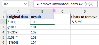
Custom function with hardcoded characters
If you do not want to bother about supplying special characters for each formula, you can specify them directly in the code:
+-» For index = 1 To Len(chars) str = Replace(str, Mid(chars, index, 1), «» ) Next RemoveSpecialChars = str End Function
Please keep in mind that the above code is for demonstration purposes. For practical use, be sure to include all the characters you want to delete in the following line:
This custom function is named RemoveSpecialChars and it requires just one argument — the original string:
To strip off special characters from our dataset, the formula is:
=RemoveSpecialChars(A2) 
Remove non-printable characters in Excel
Microsoft Excel has a special function to delete nonprinting characters — the CLEAN function. Technically, it strips off the first 32 characters in the 7-bit ASCII set (codes 0 through 31).
For example, to delete nonprintable characters from A2, here’s the formula to use:
This will eliminate non-printing characters, but spaces before/after text and between words will remain. 
To get rid of extra spaces, wrap the CLEAN formula in the TRIM function:
Now, all leading and trailing spaces are removed, while in-between spaces are reduced to a single space character: 
If you’d like to delete absolutely all spaces inside a string, then additionally substitute the space character (code number 32) with an empty string:
=TRIM(CLEAN((SUBSTITUTE(A2, CHAR(32), «»)))) 
Some spaces or other invisible characters still remain in your worksheet? That means those characters have different values in the Unicode character set.
For instance, the character code of a non-breaking space ( ) is 160 and you can purge it using this formula:
To erase a specific non-printing character, you need to find its code value first. The detailed instructions and formula examples are here: How to remove a specific non-printing character.
Delete special characters with Ultimate Suite
Supports Excel for Microsoft 365, Excel 2019 — 2010
In this last example, let me show you the easiest way to remove special characters in Excel. With the Ultimate Suite installed, this is what you need to do:
- On the Ablebits Data tab, in the Text group, click Remove >Remove Characters.

- On the add-in’s pane, pick the source range, select Remove character sets and choose the desired option from the dropdown list (Symbols & punctuation marks in this example).
- Hit the Remove button.

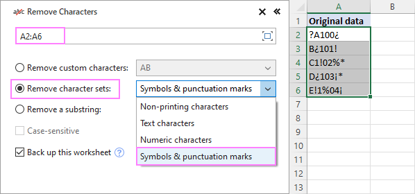
In a moment, you will get a perfect result: 
If something goes wrong, don’t worry — a backup copy of your worksheet will be created automatically as the Back up this worksheet box is selected by default.
Curious to try our Remove tool? A link to the evaluation version is right below. I thank you for reading and hope to see you on our blog next week!
Источник
Cleaning text data is often the most time-consuming task for many Excel users.
Unless you’re among the few lucky ones, you’ll most likely get your data in a format that would need some cleaning.
One common use case of this would be when you get a dataset and you have to remove some characters from the left for this dataset.
These could be a fixed number of characters that you need to remove from the left, or could be before a specific character or string.
In this tutorial, I will show you some simple examples of removing the required number of characters from the left of a text string.
Removing Fixed Number of Characters from the Left
If you get a dataset that is consistent and follow the same pattern, then you can use the technique shown here to remove a fixed number of characters from the left of the string in each cell.
Below I have a dataset where I have the product ids, which consist of a two-letter code followed by a number, and I want to extract only the number in each cell (which means that I want to remove the first three characters from each cell).

Below is the formula to do this:
=RIGHT(A2,LEN(A2)-3)

The above formula uses the LEN function to get the total number of characters in the cell in column A.
From the value that we get from the LEN function, we subtract 3, as we only want to extract the numbers and want to remove the first three characters from the left of the string in each cell.
This value is then used within the RIGHT function to extract everything except the first three characters from the left.
Since we have hardcoded the number of characters we want to remove from the left, this method would only work when you always want to remove the fixed number of characters from the left. If, in the above example, we have inconsistent data where there are varying numbers of characters before the number, we would not be able to use the above formula (use the formula next section in such a scenario).
Removing Characters from the Left based on Delimiter (Space, Comma, Dash)
In most cases, you’re unlikely to get consistent data where the number of characters you want to remove from the left would be of fixed length.
For example, below I have the names dataset where I want to remove the first name and only get the last name.

And as you can see, the length of the first name varies, so I can not use the formula covered in the previous section.
In this case, I still need to rely on a consistent pattern – which would be a space character that separates the first and the last name.
If I can remove everything till the space character, I would get the desired result.
And thanks to awesome functionalities in Excel, there are multiple ways to do this.
Using the RIGHT Formula
Let’s first have a look at a formula that will remove everything before the space character and you will be left with the last name only.
=RIGHT(TRIM(A2),LEN(TRIM(A2))-FIND(" ",TRIM(A2)))

The above formula will remove everything to the left of the space character (including the space character), and you will get the rest of the text (last name in this example).
Let me quickly explain how this formula works.
First, I have used the FIND function to get the position of the space character in the cell.
In the above formula, FIND(” “,TRIM(A2))) would return 6 as the space character occurs at the sixth position in the name in cell A2.
I then used the LEN function and subtracted the value that the FIND function gave me to get the total number of characters after the space character in the cell.
And now that I know how many characters to extract from the right of the text string, I’ve used the RIGHT function to extract it.
Note: In the above formula, I have used the TRIM function to make sure that any leading, trailing, or double spaces are taken care of.
One big benefit of using a formula is that the results automatically update in case you make any changes in the data in Column A.
Using Flash Fill
Another really fast way to quickly remove text from the left of the delimiter is by using Flash Fill.
Flash Fill works by identifying patterns from a couple of inputs from the user. In our example, I would have to manually enter the expected result for one or two cells, and then I can use Flash Fill to follow the same pattern for all the other remaining cells.
Suppose I have a dataset as shown below where I want to remove all the characters before the space character.
Below are the steps to use flash fill to remove characters from the left of a delimiter:
- In cell B2, enter the expected result (Baker in this case)

- Select cells B2 to B12 (the range where you want the result)

- Hold the Control key and press the E key (or Command + E if using Mac)

The above steps would remove everything from the left of the space character and you will be left only with the last name.
Note that Control + E (or Command + E in Mac) is the keyboard shortcut for Flash Fill in Excel.
Now let me quickly explain what’s happening here.
When I manually enter the expected result in cell B2, and then select all the cells and use Flash Fill, it tries to identify the pattern using the result I’ve already entered in cell B2.
In this example, it was able to identify that I am trying to extract the last name, which means that I’m trying to remove everything which is there on the left of the last name.
Once it was able to identify this pattern, it applied it to all the cells in the column.
In some cases, it is possible that Excel will not be able to identify the correct pattern when using Flash Fill. In such situations, you can try entering the results in more than one cell so that excel has more data to understand the pattern.
For example, you can enter the expected result in cells B2 and B3 and then select the entire column and use Flash Fill.
You can also find the Flash Fill option in the Home tab –> Editing –> Fill –> Flash Fill.
Note that in case your original data in column A changes, you will have to repeat the steps again to remove the characters before the delimiter. Unlike the formula method, this method gives a static result that doesn’t auto-update
Using Text to Columns
Another quick way to remove all the characters before a delimiter would be by using the Text to Columns feature.
Suppose I have the dataset as shown below and I want to remove everything before the dash.

Below are the steps to do this:
- Select the range that has the data (A2:A10 in this example)
- Click the ‘Data’ tab

- In the Data Tools group, click on ‘Text to Columns’

- In the Text to Columns Wizard Step 1 of 3: Make sure Delimited is selected

- Step 2 of 3: Select Other as the Delimiter, and enter – in the box next to it

- Step 3 of 3: Select the ‘Do Not Import Column (Skip)’ option. Also make sure that in the Data Preview, the column selected (in black) is the one that you want to remove.

- Step 3 of 3: In Data Preview, select the second column (the one that you want), and then select the destination cell (I will go with the already selected B2)

- Click on Finish

The above steps would split into separate columns based on the specified delimiter.
Note that in this example, I have used a delimiter to split the data into separate columns. You can also use Text to Columns to remove a specific number of characters from the left of a text string as well. For that, you should choose Fixed Length instead of the Delimiter option in Step 1 of 3 in the Text to Columns wizard.
Note that in case your original data in column A changes, you will have to repeat the steps again to remove the characters before the delimiter. Unlike the formula method, this method gives a static result that doesn’t auto-updates
Also read: How to Remove Dashes (-) in Excel?
Remove All Text On the Left of a Specific String
Sometimes, you may have a dataset where you need to get rid of all the text before a specific text string.
For example, below I have a data set where I have employees’ names followed by their telephone numbers.

I want to extract only the telephone number from each cell, which means that I want to remove everything which is before the telephone number.
As with most data cleaning methods in Excel, I need to look for a pattern that I can use to get rid of everything before the phone number.
In this case, it’s the text string ‘Tel:’.
So all I need to do is find the location of the string ‘Tel:’ in each cell, and remove everything before it (including it).
While you can build an advanced formula in Excel for this, let me show you a really cool way using Find and Replace method.
Below are the steps to remove all the text before a specific text string:
- Copy the data from column A to Column B. I am doing this so that I will get the result in column B, while still keeping the original data in column A
- Select all the cells in column B

- Hold the Control key and press the H key (Command + H if using Mac). This will open the Find and Replace dialog box.

- In the ‘Find what’ field, enter *Tel:

- Leave the ‘Replace with’ field empty

- Click on Replace All
The above steps would remove everything before the string ‘Tel:’, and you will be left with the phone number only.

How does this work?
In the above example, I have used a wild card character – asterisk (*).
Since I wanted to remove everything to the left of the string ‘Tel:’, I added an asterisk before it and used it in the ‘Find what’ field.
An asterisk (*) is a wild card character that can represent any number of characters in Excel.
This means that when I ask Excel to find ‘*Tel:’, It is going to look for the string ‘Tel:’ in each cell, and if it finds this string in any cell, no matter its position, everything up to that point would be considered while replacing the text.
And since I replaced this with nothing (by leaving the ‘Replace with’ field empty), it simply removes everything up to that string in the cell.
This means that I’m only left with the characters after that text string and everything before that text string including that string itself is removed.
Remove All Text from the Left (and keep the numbers)
Sometimes you may get a data set where you have the text and numbers together in one single cell, as shown below, and you want to remove all the text but keep the numbers only.

This can easily be done using a simple formula.
Below is the formula that would remove all the text from the left of the numbers, so that you’re only left with the number part of the string.
=RIGHT(A2,LEN(A2)-MIN(IFERROR(FIND({0,1,2,3,4,5,6,7,8,9},A2),LEN(A2)))+1)

The above formula would remove all the text portions from the left part of the cell so that you’re only left with the numbers.
Now let me quickly explain how this formula works.
The FIND({0,1,2,3,4,5,6,7,8,9},A2) part of the formula would look for these 10 digits in the cell and would return the position of these digits as an array.
For example, for sale A2 the result returned by this formula would be {8,#VALUE!,#VALUE!,#VALUE!,6,#VALUE!,#VALUE!,#VALUE!,#VALUE!,7}
As you can see, it returns 10 values where each value would represent the position of that number in the cell.
Since the digit 0 occurs at the eighth position, the first value returned is 8, and since the cell does not contain the digit 1, it returns a Value error.
Similarly, all the digits are analyzed and a number is returned if the digit is present in the cell, and the value error is returned if that digit is not in the cell.
Now, this FIND formula is wrapped within the IFERROR formula, so that instead of the value error we get something more meaningful.
In this case, the IFERROR formula would return a number when it finds the digit in the cell, and in case it does not find the digit, it would return the maximum length of the characters in the cell (which is done using the LEN formula)
This is done to make sure that in case there are cells where there are no numbers, the IFERROR formula would still return a digit that can be used in the formula (else it would have returned an error).
Now with these arrays of numbers, I have used the MIN function to find out the minimum value in that array. this would tell me the starting position where the numbers start in the cell.
For example in cell A2, it would give me 6 which means that the text part in the cell ends at the 5th character and the numbers begin from the 6th character onwards.
Now that I know at what position the numbers start in the cell, I need to know how many characters from the left I need to remove.
To do this, I have again used the LEN function to find the total length of characters in a cell, and from this, I have subtracted the result of the main function so that I would know how many text characters are there in the left.
Note that I have also subtracted 1 as I want to exclude the first number in the cell (if I don’t subtract 1 in this formula, it would also remove the first number along with the text).
And finally, I have used the RIGHT function to extract all the numbers from the right, which essentially means that all the text characters on the left are removed.
Remove All Numbers From the Left
In the previous section, I showed you how to remove all the text characters from the left so that we are only left with the numbers in the cell.
But what if the situation is reversed.
What if I have a data set as shown below where I want to remove all the numbers from the left and keep all the text characters.

We can use a similar formula with some tweaks.
Below is the formula that would remove all the numbers on the left so that you only get the text part of the cell.
=MID(A2,MIN(IFERROR(FIND({"a","b","c","d","e","f","g","h","i","j","k","l","m","n","o","p","q","r","s","t","u","v","w","x","y","z"},LOWER(A2)),LEN(A2))),1000)

While this formula may look bigger and a little scarier than the previous one, the logic is exactly the same.
In this formula, we have used the FIND function to find out the position of all the 26 alphabets in the English language.
The FIND portion of the formula checks the cell and gives us the position of each of the 26 alphabets.
Note that I have also used LOWER(A2) instead of A2, because the alphabet that I’m using in the FIND formula is in lower case.
I have then wrapped the fine formula within IFERROR, so that in case the formula is not able to find the position of a specific alphabet, instead of returning the value error, it would return the length of the content in the cell (which is given by the LEN formula).
This is to make sure that in case I have a cell where there there is no text portion there are only numbers, I would still get a numeric value.
I then used the MIN function to find out the minimum position where the text starts.
This would tell me where the numbers would end and where the text starts so that I can split the content of the cell to remove all the numbers from the left and keep the text portion.
Now that I know where the text characters start in the cell, I have used the MID function to extract everything starting from that position till the end.
Note that I have used 1000 characters to be extracted within the mid function, but in case your cell has less number of characters, only that much would be extracted.
So these are some of the examples where we have removed characters from the left in a cell in Excel.
I have shown you formulas to remove a fixed number of characters from the left or remove the characters on the left based on a delimiter.
I also showed you how to use a simple find and replace technique to remove all the characters on the left before a specific string.
And then finally I showed you two formulas that you can use to remove only the numbers or only the text from the left.
I hope you found this Excel tutorial useful.
Other Excel tutorials you may also like:
- How To Remove Text Before Or After a Specific Character In Excel
- How to Remove the First Character from a String in Excel (Quick & Easy)
- How to Combine First and Last Name in Excel (4 Easy Ways)
- How to Extract the First Word from a Text String in Excel
- Separate First and Last Name in Excel (Split Names Using Formulas)
- How to Capitalize First Letter of a Text String in Excel (using Formula & VBA)
- How to Extract a Substring in Excel (Using TEXT Formulas)