Remove cells from excel

AutoFill yes AutoFill Custom and Alphabetic Lists AutoFill Dates or Months AutoFill Numbers AutoFill Numbers Without Dragging Auto-Number Rows in a Column Fill Column With Same Value Fill Down or Fill Right Make a List of Numbers Turn Off AutoFill Turn On AutoFill Use Fill Handle Use Flash Fill to Fill a Range AutoSave yes Recover a Deleted File Recover a File That Was Not Saved Set Up AutoSave Location and Time Turn On or Off AutoSave and AutoRecover Calculation yes Add Values to Cells and Columns Anchor a Cell Change the Signs of Values Divide Cells and Columns Keep Variable Cell Constant Lock Cell in Formula Multiply Cells and Columns Stop Auto Calculation Subtract Cells and Columns Comments yes Copy Comments Delete All Comments Edit Comments Insert a Comment or Note to a Cell Show or Hide All Comments Compare yes Compare Two Columns and Highlight Differences Compare Two Columns for Matches Compare Two Files for Differences Compare Two Rows Compare Two Sheets for Differences Conditional Formatting yes Apply Conditional Formatting Based on Adjacent Cell Apply Conditional Formatting Multiple Sheets Apply Conditional Formatting to Dates Apply Conditional Formatting to Entire Column Apply Conditional Formatting to Multiple Rows Conditional Format Greater Than Or Less Than Conditional Formatting Based on Another Cell Conditional Formatting Based on Cell Value Conditional Formatting Based on Date Conditional Formatting Based on Formula Conditional Formatting Dates Overdue Conditional Formatting Formulas Not Working Conditional Formatting Grayed Out Conditional Formatting If Between Two Numbers Conditional Formatting If Cell Contains Any Text Conditional Formatting Not Equal Conditional Formatting Tips for 2023 Conditional Formatting With Multiple Conditions Copy Conditional Formatting Edit Conditional Formatting Formatting If Cell Contains Specific Text Highlight a Cell if Specific Value Exists in Another Column Highlight Blank Cells Highlight Cells If Highlight Cells That Begin or End With Highlight Duplicate Rows Highlight Duplicate Values Highlight Entire Row Highlight Every Other Line In Excel Highlight Rows If Highlight Rows That Contain Highlight the Highest Value If Formula to Set Cell Color Insert Harvey Balls Remove Conditional Formatting Use Comparison Icon Sets Use Conditional Formatting With Checkbox Use Custom Icon Sets Copy & Paste yes Copy a Cell From Another Sheet Copy a Page Copy and Paste a Range or Object as a Picture Copy and Paste an Exact Formula Copy and Paste as Text or Value Copy and Paste Cells Copy and Paste Columns Copy and Paste Formulas Between Excel and Google Sheets Copy and Paste Hyperlinks Copy and Paste Merged Cells Copy and Paste With Skip Blanks Copy and Paste Without Borders Copy and Paste Without Changing the Format Copy Cell Formatting Copy Data From One Cell to Another Automatically Copy Every Other Row Copy Formula Down to Entire Column Copy Number Not Formula Copy Value to Another Cell With Formula Drag and Drop Duplicate Rows Freeze Random Numbers Paste and Match Destination Formatting Paste Horizontal Data Vertically Paste Into Filtered Cells Rearrange Columns Replace Formula With Value Swap Cells Swap or Move Columns Transpose Rows to Columns Data Validation yes 10 Data Validation Rules and Techniques Add a ToolTip Change Data Validation Clear Data Validation Copy Data Validation Create an Input Message Data Validation Based on Another Cell Date and Time Data Validation Formats Enable Error Alert Find Restricted Values Ignore Blanks in Data Validation Restrict Cell Values Set a Character Limit Validate Phone Number Format Database yes Clean Up Data Create a Searchable Database Drop-Down List yes Add Drop-Down List With Color Formatting Alphabetize a Drop-Down List AutoComplete With Data Validation Change a Drop-Down List Create a Cascading Drop-Down List Create a Default Value for a Drop-Down List Create a Drop-Down List Create a Drop-Down List Filter Create a Yes or No Drop Down Create Drop Down Data Entry Form Create Dynamic Drop Down From Table Data Validation Unique Values Drop Down Populates Another Cell Drop-Down List With If Statement Make Drop-Down Categories and Subcategories Remove a Drop-Down List Update a Drop-Down List Duplicates yes Clear Duplicate Cells Combine Duplicate Rows Count Duplicate Values Only Once Distinct (Unique) Values Duplicates Find Duplicate Values Merge Lists Without Duplicates Paste Unique Values Prevent Duplicate Entries Remove Both Duplicates Remove Duplicate Rows Remove Unique Values Show Only Duplicates Email yes Copy Email Addresses to Outlook Email a Spreadsheet Email Address Format Validation Embed a File Send Email With Formula Send Mass Email From a List Filters yes Advanced Filter Apply Multiple Filters Clear All Filters Copy Filtered Data Delete Filtered Rows Filter by Color Filter by Date Filter Duplicate Values Filter Merged Cells Filter Rows Filter Unique Values Hide Blank Rows Hide Rows Based on Cell Value Horizontal Filter Remove Filters Save Filtered Data Show or Hide AutoFilter Arrows Show Rows With Specific Text Use Custom AutoFilters Find & Select yes Deselect Cells Fill Blank Cells With Value Above Find and Delete Words Find and Highlight Find and Replace Multiple Values Find and Replace With Wildcards Find and Select Specific Cells Find Blank Cells Find Errors Find Merged Cells Find Unique Values Highlight Blank Cells Highlight Multiple Rows Jump to a Row With Go To Remove Asterisks Replace Blank Cells With Zeros Replace Space With Underscore Search All Sheets Select All Cells With Values Select Every Other Row Select Multiple Cells Select Non-Adjacent Cells or Columns Use Go To Special Use the Go To Command to Jump to a Cell Forecast yes Add Goal Seek to Google Sheets Automatically Vary the Contents of a Cell Calculate the Break-Even Analysis Point Calculate Total Revenue Do a Sensitivity Analysis Enable Solver Add-In Insert Line and Column Sparklines Install the Data Analysis Toolpak for PC and Mac Quick Analysis Tool Remove Solver Solve for a Variable Format Cells yes Add Border Lines Alternate Row Color Apply and Change Themes Apply Cell Styles AutoFit Columns Automatic Formatting Cell Margins Change Gridline or Cell Border Color Change the Cell Background Color Clear All Formatting Copy Cell Color Copy Column Widths Copy Row Height Make All Rows and Columns the Same Height and Width Merge and Center Cells Merge Multiple Cells Outline Cells Remove Filll Color Resize Cells to Default Row Height Resize Multiple Rows or Columns at Once Split a Cell Diagonally Unmerge Cells Use Format Painter for Multiple Cells Format Text yes Add and Remove Strikethrough Bold Lines Center Across Selection Change Alignment Create a Bulleted List Create Barcodes Go Down to the Next Line Hide Overflow Text in a Cell Increase Indent Line Spacing Make Cells Bigger to Fit Text Make Subscripts and Superscripts Rotate Text in a Cell Shrink to Make Text Fit Two Lines in One Cell Underline Text Word Wrap Write Paragraphs Write Text Vertically X Out a Cell Formula Auditing yes Allow Circular References Camera Tool Find a Circular Reference Error Formula View Mode Hide All Dependency Tracer Arrows at Once Hide Precedent Tracer Arrows Ignore All Errors Insert Functions With Dialog Box Show Dependent Tracer Arrows Show Precedent Tracer Arrows Use Formula AutoComplete Use the Error Checking Command Watch Window Insert & Delete yes Clear Cell Contents Delete Blank Columns Delete Blank Rows Delete Cells and Shift Cells Left Delete Cells and Shift Cells Up Delete Every Other Column Delete Every Other Row Delete Hidden Rows and Columns Delete Highlighted Cells Delete Infinite Rows or Columns Delete Multiple Cells Delete Multiple Rows or Columns Delete Rows if Cell Contains Specific Text Delete Rows With Blank Cells Insert Blank Row Insert Blank Row After Every Other Row Insert Cells and Shift Cells Down Insert Cells and Shift Cells Right Insert Multiple Rows and Columns Reset the Last Cell Links yes Break All Links Create a Hyperlink Cross-Reference Find External Links Hyperlink to Another Sheet or Workbook Link Files Mirror Cells by Linking Update Links Automatically Miscellaneous yes 32-Bit Versus 64-Bit Office Change Author Property Change Cell Size in Pixels or Inches Change Document Properties Clear the Cache Customize the Ribbon Delete a File Find the Last Saved Date Find What Version of Excel You Have Generate All Permutations Insert Timestamp Make a File Smaller Open Files in New Windows Show the Formula Bar Show the Toolbar Take a Screenshot What is the Formula Bar? Name Manager yes Create Range Names From Selection Delete Named Range Dynamic Named Range Based on Cell Edit Named Ranges Find the Location of a Named Range Paste Range Names Resolve a Name Conflict for a Named Range Use the Name Box What are Name Manager and Name Box? Number Formats yes Add a Plus Sign for Positive Add More Decimal Places Add Percentage Style to a Number Add Units to Numbers Apply Accounting Number Format Convert Date to Month and Year Convert Decimal to Fraction Display Fraction Without Reducing Format Phone Numbers With Dashes Format Time to Milliseconds Get Rid of the Dollar Sign Hide Zeros Limit Decimal Places Make Negative Numbers Red Mask Data Input Move Decimal Places Number Format in Millions Number Format in Thousands Pad Numbers With Leading Zeros Prevent Rounding Remove Decimals Remove Scientific Notation Round Numbers Without a Formula Stop Changing Numbers to Dates Use Scientific Notation Objects yes Add and Group Radio Buttons Add Gradient Fill to Shapes or Cells Change the Color of an ActiveX Control Button Circle Something Create a Shape With Drawing Tools Create a Slider Bar Delete a Checkbox Draw Lines Insert a Digital Signature Insert a Drop-Down Calendar With Date Picker Control Insert a Logo Insert a Shape Insert a SmartArt Graphic Insert a Text Box Insert an Arrow Insert Multiple Checkboxes Insert Multiple Hyperlinks in One Cell Insert Toggle Button Link a Text Box Make a Combo Box Make a Number Line Select Objects Organize Sheets yes Add Multiple Worksheets Copy a Spreadsheet Copy Multiple Sheets to a New Workbook Count Number of Worksheets Delete Multiple Tabs Delete Worksheets Group and Ungroup Worksheets Hide and Unhide Worksheets Insert a New Tab Merge Multiple Workbooks Into One Merge Two Spreadsheets Into One Pull Data From Multiple Sheets and Consolidate Rename a Worksheet Select Multiple Sheets Separate Sheets View a List of Worksheet Tabs View Two Sheets at Once Outline yes Collapse an Outline to Show Just the Subtotals Create an Outline Create Auto Outline Expand or Collapse Rows or Columns Group Cells Page Layout yes Add Element to Display Current Date in the Header Change Orientation to Landscape Create Cover Page Define Print Titles on Every Page Format the Header and Footer Insert or Remove Headers and Footers Make a Header Only on the First Page Make a Sheet Fit on One Page Scale to Fit Page Size Set Custom Page Size What is the Page Setup Function? Pictures yes Drag and Drop Pictures Insert a Background Image Insert a Picture Into a Cell Insert a Picture Into a Cell Automatically Insert a Picture Into the Header Insert Pictures Make a Picture Transparent Remove All Pictures From a Workbook Show a MouseOver Picture Pivot Table yes Add Calculated Field to Pivot Table Advanced Pivot Table Techniques Change Pivot Table Data Source Count Unique Values With Pivot Table Create Pivot Table Delete Pivot Table Filter Pivot Table Values Get a Count in Pivot Table Group Pivot Table by Date Keep Pivot Table Formatting Make a Pivot Table Chart Pivot Table Slicers Pivot Table Sorting Guide Refresh a Pivot Table Remove Field From Pivot Table Power Query yes Export Folder and Subfolder Structure Import an HTML Table Import XML Files Set Up Automatic Currency Conversion Print yes Add a Page Border Add a Watermark Center Worksheets Horizontally and Vertically Change Print Area Clear Print Area Delete Unwanted or Blank Pages Display and Print Formulas Excel Borders Not Printing Hide Page Breaks Insert a Page Number Insert and Remove Page Breaks Make Graph Paper Print Print a Background Image Print a Chart or Graph Print All Tabs in a Workbook Print Comments Print Gridlines on a Blank Sheet Print Multiple Sheets Print Only Selected Cells Print Preview Print Row Numbers and Column Headings Print Selected Worksheets on One Page Print Selected Worksheets Without Print Preview Print Two Sheets on One Page Remove Watermarks Set the Print Area Show Print Area Proofing yes Check Spelling Disable Automatic Hyperlinks Remove Hyperlinks Stop AutoCorrect Turn On or Change AutoCorrect Protect yes Change a Read Only File Hide Formulas Lock a Sheet for Viewing Lock Cells Lock Column Width and Row Height Lock Formatting Mark a Workbook as Final Password Protect a File Protect Workbook Structure Protected View: Turn Off and Enable Editing Remove a Password From a File Unlock Cells Unprotect a Workbook Save As yes Change the Default Directory Convert a CSV File to XLSX Convert a Spreadsheet to a Delimited Text File Convert an Excel File to Google Sheets Convert to a Pipe Delimited Text File Copy Entire Workbook Create a Word Document Embed Tables Into HTML Export a File to PDF Import a Word Document Open a Text File Open Old XLS Files Recover Deleted Sheet Rename a File Save a File as CSV Save a File as CSV With UTF-8 Encoding Save a File to the Old Format Save a Macro-Enabled Workbook Save a Table as an Image Save File as Read-Only Save Just One Sheet Save Multiple Sheets as a PDF Save Workbook as PDF What is the Difference Between CSV Files and Excel Files? Share Files yes Make a Shared Spreadsheet for Multiple Users Track Changes Unshare a Workbook Use Document Inspector Sort Data yes Advanced Sorting Keep Rows Together During Sort Put Things in Alphabetical Order Random Sort Reverse the Order of Data Sort a Column Alphabetically Sort and Ignore Blanks Sort by Last Name Sort By Month Sort By Number Sort Data Sort Dates in Chronological Order Sort Highlighted Cells by Color Sort IP Addresses Sort Multiple Columns Sort Multiple Rows Horizontally Sort Subtotals Sort With a Custom List Sort Without Duplicates Undo a Sort Symbols yes Add Bullet Points Division Sign Find and Replace Question Marks and Asterisks Insert a Check Mark Insert Bitcoin Symbol Insert Cent Symbol Insert Cross Text Symbol Insert Delta Symbol Insert Euro Symbol Insert Plus or Minus Symbol Insert Pound Symbol Insert Rupee Symbol Insert Signs and Symbols Insert Sum Symbol Insert Yen Symbol Star Symbol What Do the Symbols Mean in Formulas? Tables yes Add a Column and Extend a Table Add a Total or Subtotal Row to a Table Add Rows to Table Center Table Change Table Style Compare Two Tables Convert a Table to a Normal Range Convert Data to Table Copy and Paste Table Copy Table From Word Copy to Word and Fit Page Create Floating Table Create Lookup Table Create Table Display Data With Banded Rows Flip a Table Link Tables Make Columns Sortable Move Table Paste Excel Table Into Gmail Remove a Table or Table Formatting Rename a Table Rotate Data Tables Table Tools Types of Tables Text to Columns yes Convert String to Date Paste CSV Data Into Columns Separate Numbers Split a Cell Into Two or More Columns Split a Text Cell to Two or More Rows Use a Line Break in Text to Columns Use Text to Columns to Parse Data Troubleshooting yes #REF Error Advance Filter Not Working Command Cannot be Used on Multiple Selections Data Validation Not Working Excel Cannot Open or Save Any More Documents Excel Cannot Paste the Data Error Excel Not Sorting Numbers Correctly Fill Series Not Working Find Broken Links Fix Excel Find Not Working Fix the #NAME? Error Get Rid of Green Triangle Get Rid of the Red Triangle in Google Sheets Loading Solver Not Working Printing Problems Printing Too Small Solver Encountered Error Value The Pivot Table Field Name Is Not Valid There Isn’t Enough Memory to Complete This Action Waiting for OLE Action Error What to Do When Excel Keeps Crashing or Freezing Why is AutoSave Not Working or Grayed Out? View yes Close Header and Footer Dark Mode Enable and Disable Smart Tags Freeze and Unfreeze Panes Get Rid of Dashed Print Area Lines Hide and Unhide Rows and Columns Hide and Unhide Workbooks Hide Column and Row Headings Hide Unused Cells Hide Vertical and Horizontal Scroll Bars Lock Columns Lock the Top Row When Scrolling Remove Page Number in Preview Mode Return to Normal View Show and Hide Gridlines Show or Hide ScreenTips Show the Ruler Use Split Screen View Full Screen View Header Zoom In or Out Excel Built-in Charts yes Column Charts: Stacked, Clustered Bar Charts: Stacked, Clustered Area Charts Line Charts Candlestick Charts Pareto Chart Waterfall Chart Sales Funnel Chart Advanced Custom Charts yes Gauge / Dial Chart Tornado Chart Burndown Chart Step Chart Thermometer Chart Quadrant Chart Bullet Chart Ogive Chart Bell Curve / Normal Distribution Plot Stem & Leaf Chart Mekko Chart Venn Diagram Polar Plot Venn Diagram Panel Chart Timeline Chart Progress Charts Sales Funnel Chart Floating Bar Chart Forest Plot Frequency Polygon Arrow Chart Percentage Graph Time Series Graph Percentage Change Chart Show Percentage in Pie Chart Dot Plot Q-Q Plot Log-Log Plot Normal Probability Plot Charts Tips & Tricks yes Add or Move Data Labels Add Data Series Add Average Line Add Data Points Add Error Bars Add Gridlines Add Line of Best Fit Add Title Break Chart Axis Calculate Area Under Curve Plot Residuals Change Bar Chart Width Change Chart Colors Chart Axis Text Instead of Numbers Copy Chart Format Create Chart with Date or Time Curve Fitting Export Chart as PDF Add Axis Labels Add Secondary Axis Change Chart Series Name Change Horizontal Axis Values Create Chart in a Cell Graph an Equation or Function Overlay Two Graphs Plot Multiple Lines Rotate Pie Chart Switch X and Y Axis Insert Textbox Move Chart to New Sheet Move Horizontal Axis to Bottom Move Vertical Axis to Left Remove Gridlines Reverse a Chart Rotate a Chart Rounded Corners or Shadows Create, Save, & Use Excel Chart Templates Dynamic Chart Titles Chart Conditional Formatting Dynamic Chart Range Animated Charts Interactive / Dynamic Charts

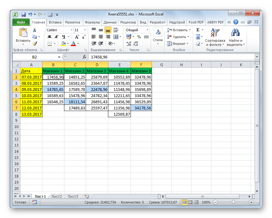
При работе с таблицами Excel довольно часто нужно не только вставить ячейки, но и удалить их. Процедура удаления, в общем, интуитивно понятна, но существует несколько вариантов проведения данной операции, о которых не все пользователи слышали. Давайте подробнее узнаем обо всех способах убрать определенные ячейки из таблицы Excel.

Читайте также: Как удалить строку в Excel

Процедура удаления ячеек

Собственно, процедура удаления ячеек в Excel обратна операции их добавления. Её можно подразделить на две большие группы: удаление заполненных и пустых ячеек. Последний вид, к тому же, можно автоматизировать.

Важно знать, что при удалении ячеек или их групп, а не цельных строк и столбцов, происходит смещение данных в таблице. Поэтому выполнение данной процедуры должно быть осознанным.

Способ 1: контекстное меню

Прежде всего, давайте рассмотрим выполнение указанной процедуры через контекстное меню. Это один и самых популярных видов выполнения данной операции. Его можно применять, как к заполненным элементам, так и к пустым.

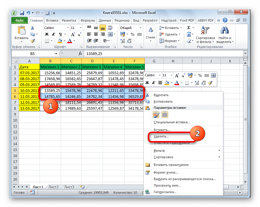
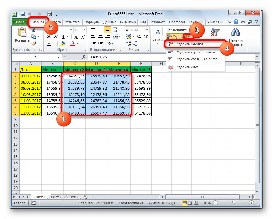
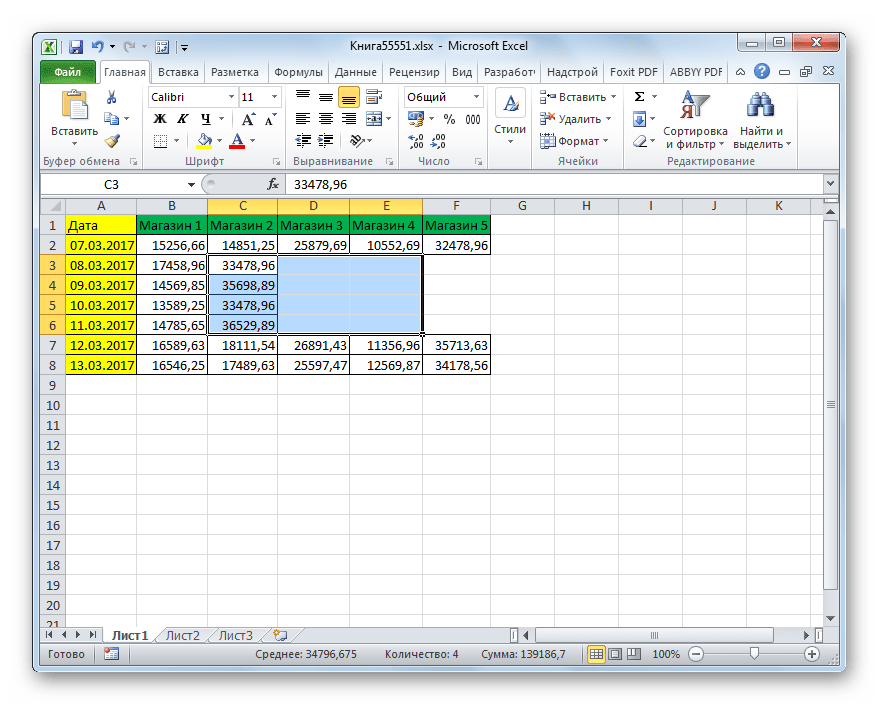
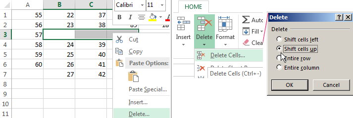
1. Выделяем один элемент или группу, которую желаем удалить. Выполняем щелчок по выделению правой кнопкой мыши. Производится запуск контекстного меню. В нем выбираем позицию «Удалить…».



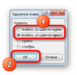
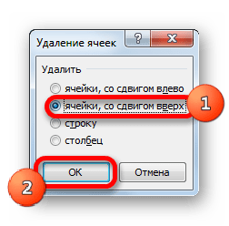
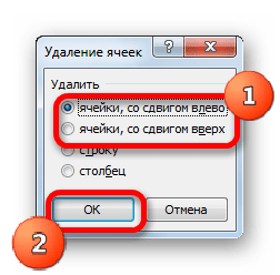
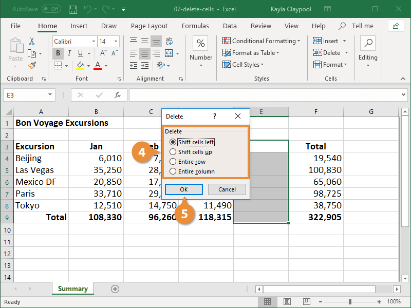
2. Запускается небольшое окошко удаления ячеек. В нем нужно выбрать, что именно мы хотим удалить. Существуют следующие варианты выбора:
   • Ячейки, со сдвигом влево;
   • Ячейки со сдвигом вверх;
   • Строку;
   • Столбец.

   Так как нам нужно удалить именно ячейки, а не целые строки или столбцы, то на два последних варианта внимания не обращаем. Выбираем действие, которое вам подойдет из первых двух вариантов, и выставляем переключатель в соответствующее положение. Затем щелкаем по кнопке «OK».



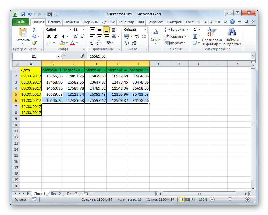
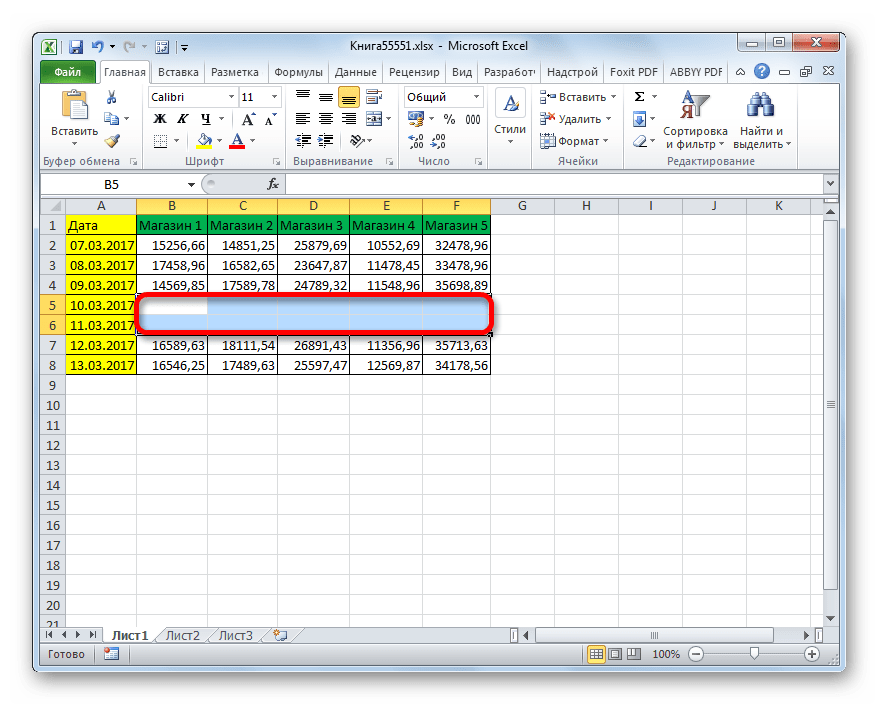
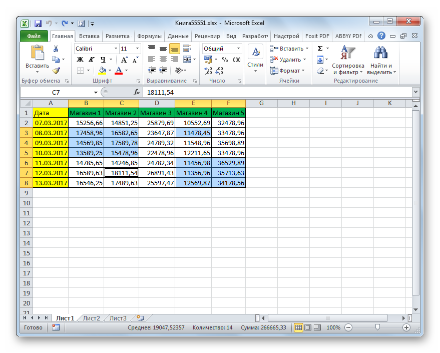
3. Как видим, после данного действия все выделенные элементы будут удалены, если был выбран первый пункт из списка, о котором шла речь выше, то со сдвигом вверх.

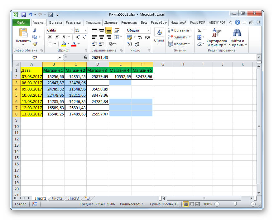
А, если был выбран второй пункт, то со сдвигом влево.

Способ 2: инструменты на ленте

Удаление ячеек в Экселе можно также произвести, воспользовавшись теми инструментами, которые представлены на ленте.

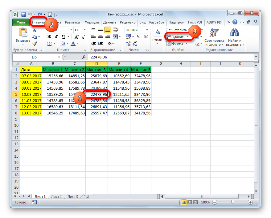
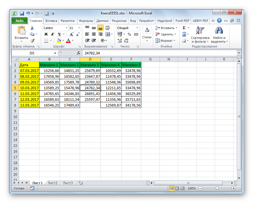
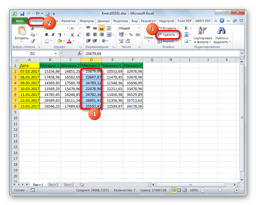
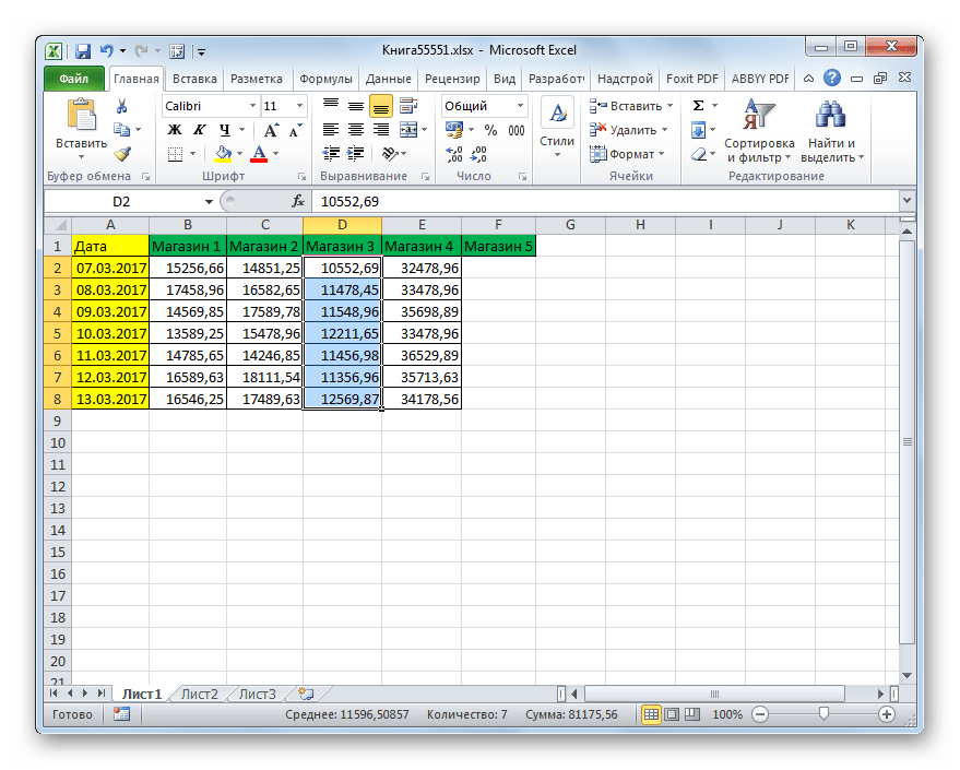
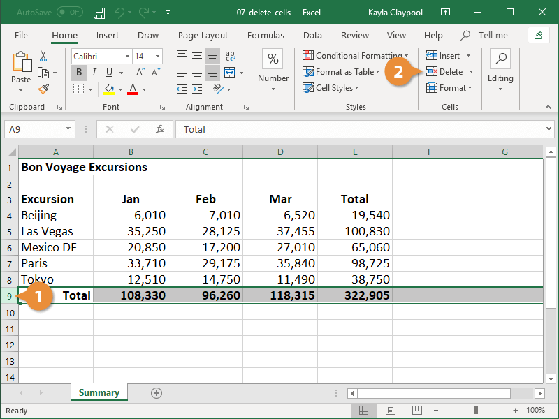
1. Выделяем элемент, который следует удалить. Перемещаемся во вкладку «Главная» и жмем на кнопку «Удалить», которая располагается на ленте в блоке инструментов «Ячейки».



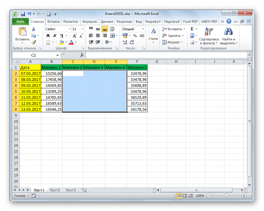
2. После этого выбранный элемент будет удален со сдвигом вверх. Таким образом, данный вариант этого способа не предусматривает выбора пользователем направления сдвига.

Если вы захотите удалить горизонтальную группу ячеек указанным способом, то для этого будут действовать следующие правила.

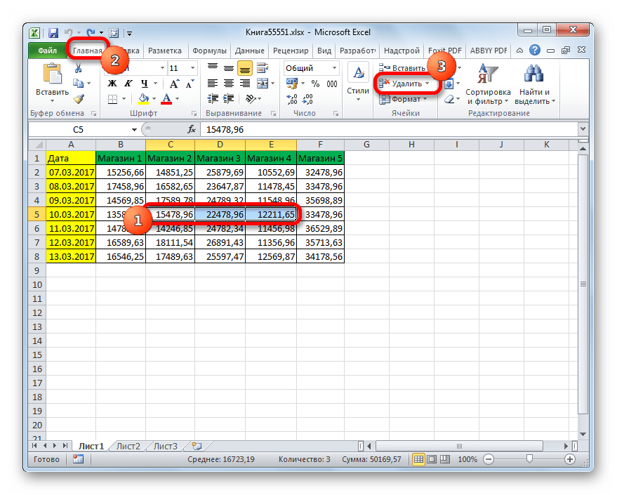
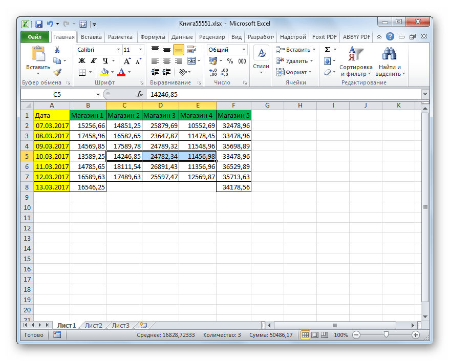
1. Выделяем эту группу элементов горизонтальной направленности. Кликаем по кнопке «Удалить», размещенной во вкладке «Главная».



2. Как и в предыдущем варианте, происходит удаление выделенных элементов со сдвигом вверх.

Если же мы попробуем удалить вертикальную группу элементов, то сдвиг произойдет в другом направлении.

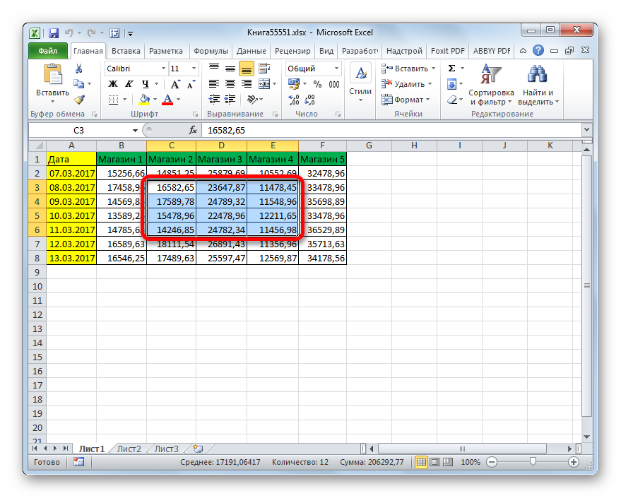
1. Выделяем группу элементов вертикальной направленности. Производим щелчок по кнопке «Удалить» на ленте.



2. Как видим, по завершении данной процедуры выбранные элементы подверглись удалению со сдвигом влево.

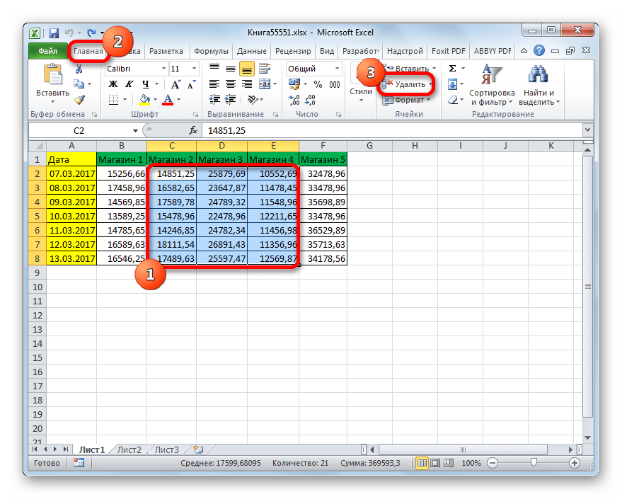
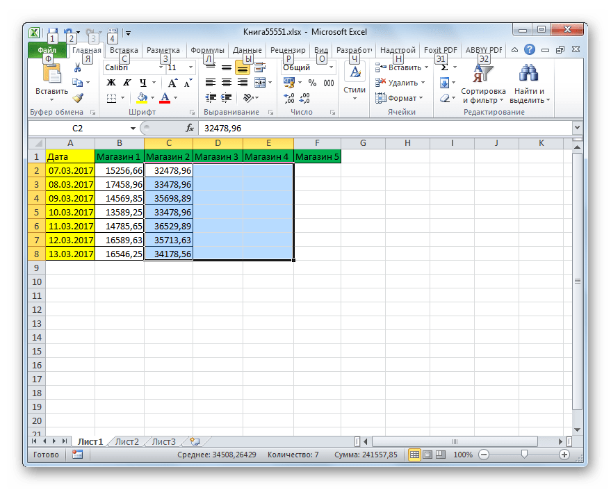
А теперь попытаемся произвести удаление данным способом многомерного массива, содержащего элементы, как горизонтальной, так и вертикальной направленности.

1. Выделяем этот массив и жмем на кнопку «Удалить» на ленте.



2. Как видим, в этом случае все выбранные элементы были удалены со сдвигом влево.

Считается, что использование инструментов на ленте менее функционально, чем удаление через контекстное меню, так как данный вариант не предоставляет пользователю выбора направления сдвига. Но это не так. С помощью инструментов на ленте также можно удалить ячейки, самостоятельно выбрав направление сдвига. Посмотрим, как это будет выглядеть на примере того же массива в таблице.

1. Выделяем многомерный массив, который следует удалить. После этого жмем не на саму кнопку «Удалить», а на треугольник, который размещается сразу справа от неё. Активируется список доступных действий. В нем следует выбрать вариант «Удалить ячейки…».



2. Вслед за этим происходит запуск окошка удаления, которое нам уже знакомо по первому варианту. Если нам нужно удалить многомерный массив со сдвигом, отличным от того, который происходит при простом нажатии на кнопку «Удалить» на ленте, то следует переставить переключатель в позицию «Ячейки, со сдвигом вверх». Затем производим щелчок по кнопке «OK».



3. Как видим, после этого массив был удален так, как были заданы настройки в окне удаления, то есть, со сдвигом вверх.

Способ 3: использование горячих клавиш

Но быстрее всего выполнить изучаемую процедуру можно при помощи набора сочетания горячих клавиш.

1. Выделяем на листе диапазон, который желаем убрать. После этого жмем комбинацию клавиш «Ctrl»+»-« на клавиатуре.



2. Запускается уже привычное для нас окно удаления элементов. Выбираем желаемое направление сдвига и щелкаем по кнопке «OK».



3. Как видим, после этого выбранные элементы были удалены с направлением сдвига, которое было указано в предыдущем пункте.

Урок: Горячие клавиши в Экселе

Способ 4: удаление разрозненных элементов

Существуют случаи, когда нужно удалить несколько диапазонов, которые не являются смежными, то есть, находятся в разных областях таблицы. Конечно, их можно удалить любым из вышеописанных способов, произведя процедуру отдельно с каждым элементом. Но это может отнять слишком много времени. Существует возможность убрать разрозненные элементы с листа гораздо быстрее. Но для этого их следует, прежде всего, выделить.

1. Первый элемент выделяем обычным способом, зажимая левую кнопку мыши и обведя его курсором. Затем следует зажать на кнопку Ctrl и кликать по остальным разрозненным ячейкам или обводить диапазоны курсором с зажатой левой кнопкой мыши.



2. После того, когда выделение выполнено, можно произвести удаление любым из трех способов, которые мы описывали выше. Удалены будут все выбранные элементы.

Способ 5: удаление пустых ячеек

Если вам нужно удалить пустые элементы в таблице, то данную процедуру можно автоматизировать и не выделять отдельно каждую из них. Существует несколько вариантов решения данной задачи, но проще всего это выполнить с помощью инструмента выделения групп ячеек.

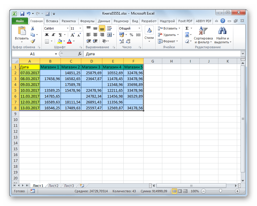
1. Выделяем таблицу или любой другой диапазон на листе, где предстоит произвести удаление. Затем щелкаем на клавиатуре по функциональной клавише F5.



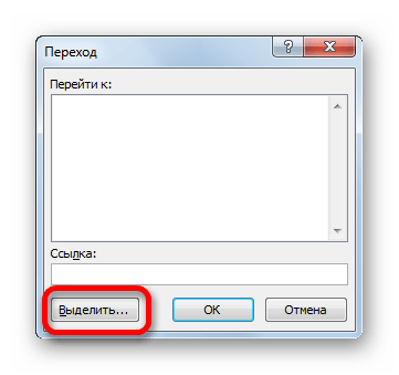
2. Запускается окно перехода. В нем следует щелкнуть по кнопке «Выделить…», размещенной в его нижнем левом углу.



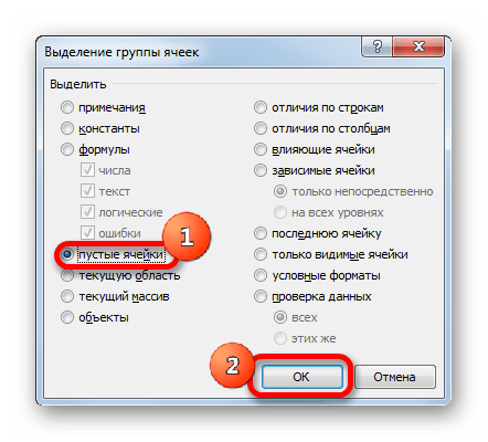
3. После этого открывается окно выделения групп ячеек. В нем следует установить переключатель в позицию «Пустые ячейки», а затем щелкнуть по кнопке «OK» в нижнем правом углу данного окна.



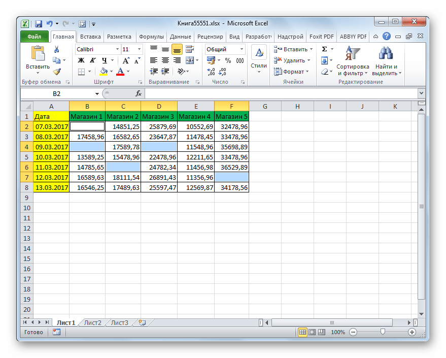
4. Как видим, после выполнения последнего действия все пустые элементы в указанном диапазоне были выделены.



5. Теперь нам остается только произвести удаление этих элементов любым из вариантов, которые указаны в первых трех способах данного урока.

Существуют и другие варианты удаления пустых элементов, более подробно о которых говорится в отдельной статье.

Урок: Как удалить пустые ячейки в Экселе

Как видим, существует несколько способов удаления ячеек в Excel. Механизм большинства из них идентичен, поэтому при выборе конкретного варианта действий пользователь ориентируется на свои личные предпочтения. Но стоит все-таки заметить, что быстрее всего выполнять данную процедуру можно при помощи комбинации горячих клавиш. Особняком стоит удаление пустых элементов. Данную задачу можно автоматизировать при помощи инструмента выделения ячеек, но потом для непосредственного удаления все равно придется воспользоваться одним из стандартных вариантов.

Insert or delete rows and columns

Insert and delete rows and columns to organize your worksheet better.

Note: Microsoft Excel has the following column and row limits: 16,384 columns wide by 1,048,576 rows tall.

Insert or delete a column

1. Select any cell within the column, then go to Home > Insert > Insert Sheet Columns or Delete Sheet Columns.

2. Alternatively, right-click the top of the column, and then select Insert or Delete. 

Insert or delete a row

1. Select any cell within the row, then go to Home > Insert > Insert Sheet Rows or Delete Sheet Rows.

2. Alternatively, right-click the row number, and then select Insert or Delete.

Formatting options

When you select a row or column that has formatting applied, that formatting will be transferred to a new row or column that you insert. If you don’t want the formatting to be applied, you can select the Insert Options button after you insert, and choose from one of the options as follows:

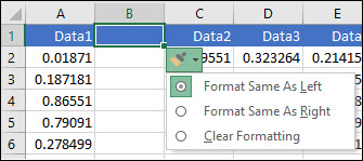
If the Insert Options button isn’t visible, then go to File > Options > Advanced > in the Cut, copy and paste group, check the Show Insert Options buttons option.

Insert rows

To insert a single row: Right-click the whole row above which you want to insert the new row, and then select Insert Rows.

To insert multiple rows: Select the same number of rows above which you want to add new ones. Right-click the selection, and then select Insert Rows.

Insert columns

To insert a single column: Right-click the whole column to the right of where you want to add the new column, and then select Insert Columns.

To insert multiple columns: Select the same number of columns to the right of where you want to add new ones. Right-click the selection, and then select Insert Columns.

Delete cells, rows, or columns

If you don’t need any of the existing cells, rows or columns, here’s how to delete them:

1. Select the cells, rows, or columns that you want to delete.

2. Right-click, and then select the appropriate delete option, for example, Delete Cells & Shift Up, Delete Cells & Shift Left, Delete Rows, or Delete Columns. 

When you delete rows or columns, other rows or columns automatically shift up or to the left.

Tip: If you change your mind right after you deleted a cell, row, or column, just press Ctrl+Z to restore it.

Insert cells

To insert a single cell:

1. Right-click the cell above which you want to insert a new cell.

2. Select Insert, and then select Cells & Shift Down.

To insert multiple cells:

1. Select the same number of cells above which you want to add the new ones.

2. Right-click the selection, and then select Insert > Cells & Shift Down.

Need more help?

You can always ask an expert in the Excel Tech Community or get support in the Answers community.

See Also

Basic tasks in Excel

Overview of formulas in Excel

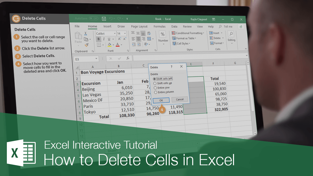
If you later decide you no longer need a group of cells, columns, or rows, you can delete them. Deleting a cell differs from clearing a cell’s content, as a “hole” is created by the deleted cell(s) and adjacent cells will move to fill that hole.

Delete Cells

1. Select the cell or cell range where you want to delete.

Pressing the Delete key only clears a cell’s contents; it doesn’t delete the actual cell.

2. Click the Delete list arrow.
3. Select Delete Cells.

   

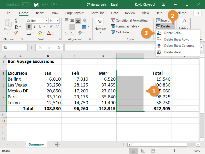
   The Delete dialog box appears.

4. Select how you want to move cells to fill in the deleted area:
   • Shift cells right: Shift existing cells to the right.
   • Shift cells down: Shift existing cells down.
   • Entire row: Delete an entire row.
   • Entire column: Delete an entire column.
5. Click OK.

   

   You can also delete cells by right-clicking the selected cell(s) and selecting Delete from the contextual menu.

The cell(s) are deleted and the remaining cells are shifted.

Delete Rows or Columns

1. Select the column or row you want to delete.
2. Click the Delete button.

   

   You can also delete cells by right-clicking the selected cell(s) and selecting Delete from the contextual menu.

The rows or columns are deleted. Remaining rows are shifted up, while remaining columns are shifted to the left.

FREE Quick Reference

Click to Download

Free to distribute with our compliments; we hope you will consider our paid training.

---

Delete Cells

Cells can be deleted by selecting them, and pressing the delete button.

Note: The delete function will not delete the formatting of the cell, just the value inside of it.

Let’s have a look at three examples.

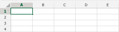
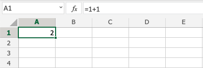
Example 1

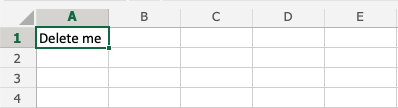
Pressing the delete button:

---

Example 2

Pressing the delete button:

---

---

Example 3

With formatting:

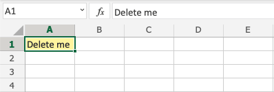
Pressing the delete button:

Note that it only deletes the value in the cells, and not the formatting (the color).

Note: You will learn more about formatting, and how to style cells in a later chapter.

---

Inserting rows and columns in Excel is very convenient when formatting tables and sheets. But function of inserting cells and entire adjacent and non-adjacent ranges enhances program features to new level.

Consider the practical examples how to add (or remove) cells and their ranges in the spreadsheet in Excel. In fact the cells are not added as the value moves on other. This fact should be taken into account when the sheet is filled with more than 50%. Then the remaining amount of cells for rows or columns may not be enough and this operation will delete the data. In such cases you should divide content of one sheet into 2 or 3 sheets. This is one of the main reasons why the new Excel version has more numbers of columns and rows (65,000 lines in the older versions and 1 000 000 in new one).



Inserting a range of empty cells

How to insert a cell in an Excel spreadsheet? Let’s say we have a table of values to which you want to insert two empty cells in between.

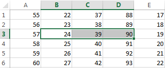
Perform the following procedure:

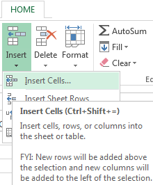
1. Select the range in the place where you need to add new empty blocks. Go to the tab «HOME» — «Insert» — «Insert Cells». Or simply right click on the highlighted area and select the paste option. Or you may press the hotkey combination CTRL + SHIFT + «+».



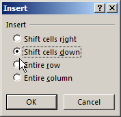
2. A «Insert» dialog box appears where it is necessary to set the required parameters. In this case select «Shift down».



3. Click OK. After that in the table with values new cells will be added. And the old will retain values and move down giving its place.

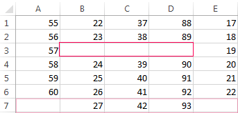
In this situation you can simply press the tool «HOME» — «Insert» (without choosing other options). Then the new cells will be inserted and the old ones will shift down (by default) without calling the dialog box options.

Use hotkeys combination CTRL + SHIFT + «plus» to add cells in Excel after selecting them.

Note. Pay attention to the settings dialog box. The last two parameters allow us to insert rows and columns in the same manner.



Removing cells

Now let’s remove the same range from our table with values. Just select the desired range. Right-click on the selected range and choose «Delete». Or go to the tab «HOME» — «Delete», «Shift up». The result is inversely proportional to the previous result.

Select the range and use shortcut keys CTRL + «negative» if you want to remove cells in Excel.

Note. Likewise you can delete rows and columns.

Attention! In practice using tools «Insert» or «Delete» while inserting or deleting ranges without window with settings should be avoided so as not to get lost in the large and complex tables. Use the hotkeys if you want to save time. They cause a dialog box with removing the paste options and it also allows you to cope with the task much quickly.

Updated: 07/31/2022 by

Below is information about how to add and remove a cell, column, or row in a Microsoft Excel spreadsheet.

Adding a cell

Note

When adding a new cell, data around the cell is moved down or to the right depending on how it’s shifted. If there is data in adjacent cells that line up with the selected cell, it becomes unaligned. In some situations, it may be better to add a new column or add a new row instead of a new cell.

To add a new individual cell to an Excel spreadsheet, follow the steps below.

1. Select the cell of where you want to insert a new cell by clicking the cell once with the mouse.
2. Right-click the cell of where you want to insert a new cell.
3. In the right-click menu that appears, select Insert.
4. Choose either Shift cells right or Shift cells down depending on how you want to affect the data around the cells.

Removing a cell

Note

When removing a cell, data around the cell is moved up or to the left depending on how it’s shifted. If there’s data in adjacent cells that line up with the selected cell, it becomes unaligned.

To remove a cell from an Excel spreadsheet, follow the steps below.

1. Right-click the cell you want to remove.
2. In the pop-up menu that appears, select Delete.
3. Choose Shift cells left or Shift cells up, depending on how you want to affect the data around the cells.

Adding a row

Excel 2007 and later

1. Select the cell where you want to add a row. For example, to add a row on the ‘3’ row, select the A3 cell or any other cell in row 3.
2. On the Home tab in the Ribbon menu, click Insert and select Insert Sheet Rows. You can also right-click the selected cell, select Insert, then select the Entire row option.

Tip

If you want to add multiple rows at once, highlight more than one row, then click Insert and select Insert Sheet Rows. For example, if you wanted to add four rows beginning at row 3, highlight row 3 and the three rows following it. Do this by clicking and dragging your mouse on the number 3, 4, 5, and 6. Then click Insert, and select Insert Sheet Rows.

Excel 2003 and earlier

1. Select the cell where you want to add a row. For example, to add a row on the ‘3’ row, select the A3 cell or any other cell in row 3.
2. In the menu bar, click Insert and select Rows. This option won’t be available if you’re highlighting columns and not rows.

Tip

If you want to add multiple rows at once, highlight more than one row and then click Insert and select Rows. For example, to add four rows beginning at row 3, highlight row 3 and the three rows following it. Do this by clicking and dragging your mouse on the number 3, 4, 5, and 6. Then, click Insert, and select Rows.

Removing a row

Excel 2007 and later

1. Highlight the row you want to delete.
2. On the Home tab in the Ribbon menu, click Delete and select Delete Sheet Rows. You can also right-click the highlighted row and select Delete.

Using the steps above, delete the row and move the rows under the deleted row up. If you want to delete the contents of the row, press Delete on the keyboard.

Excel 2003 and earlier

1. Highlight the row you want to delete.
2. In the menu bar, click Edit and select Delete. You can also right-click with your mouse on the highlighted row and select Delete.

Using the above steps, delete the row and move the rows under the deleted row up. If you want to delete the contents of the row, press Delete on the keyboard.

Adding a column

Excel 2007 and later

1. Select the cell where you want to add a column. For example, to add a column on the ‘C’ column, select the C1 cell or any other cell in column C.
2. On the Home tab in the Ribbon menu, click Insert and select Insert Sheet Columns. You can also right-click the selected cell, select Insert, then select the Entire column option.

Tip

If you want to add multiple columns at once, highlight more than one column, click Insert and select Insert Sheet Columns. For example, if you want to add four rows on column C, highlight the C column. Then, additionally highlight the three columns to the right, by clicking and dragging on the C, D, E, and F letters. Alternatively, with column C highlighted, hold Shift and click the F column header. Then click Insert and select Insert Sheet Column.

Excel 2003 and earlier

1. Select the cell where you want to add a column. For example, to add a column on the ‘C’ column, select the C1 cell or any other cell in column C.
2. In the menu bar, click Insert and select Columns. This option is not available if you’re highlighting rows and not columns.

Tip

If you want to add multiple columns at once, highlight more than one column, click Insert and select Columns. For example, if you want to add four rows on column C, highlight the C column. Then, additionally highlight the three columns to the right, by clicking and dragging on the C, D, E, and F letters. Alternatively, with column C highlighted, hold Shift and click the F column header. Then click Insert and select Column.

Removing a column

Excel 2007 and later

1. Highlight the column or columns you want to delete.
2. On the Home tab in the Ribbon menu, click Delete and select Delete Sheet Columns. You can also right-click the highlighted column and select Delete.

Using the steps above, delete the column and move the columns to the right over to the left. If you want to delete the contents of the column, press Delete on the keyboard.

Excel 2003 and earlier

1. Highlight the column or columns you want to delete.
2. In the menu bar, click Edit and select Delete. You can also right-click with your mouse on the highlighted column and select Delete.

Using the steps above, delete the column and move the columns to the right over to the left. If you want to delete the contents of the column, press Delete on the keyboard.

If there are some blank cells, rows, or columns that make your excel data seems not so easy to read or edit, you can try to delete or move them manually and accurately. But if the excel file is large, and there are several excel spreadsheets in it, probably manual deletion would waste you lots of time. So let’s learn to delete or remove blank or empty cells/rows/columns easily, even though it would probably damage your excel data.

Step 1: Select the data range you want to delete blank cells.

Step 2: In Home tab, press Ctrl + F to open Find and Replace dialog.

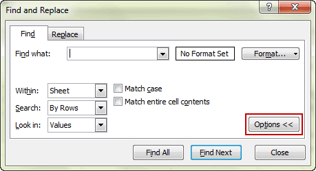
Under Find tab in Find and Replace dialog, click the Options to expand all the options you can set when you want to find something in selected excel file.

For example, if you want to find out all the blank cells in selected data range, choose to Look in “Values” and let Find what be blank. Click Find All and all the blank cells are found.

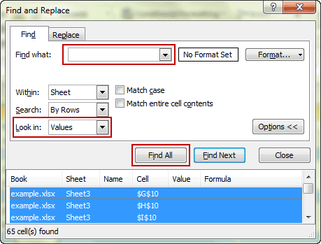
Step 3: In results you find, press Ctrl + A to select all of them and click “Delete > Delete Sheet Rows” in Home tab and Cells group.

Instantly, all of the found cells would be removed or deleted from data range.

How to delete blank rows/columns in Excel?

Two methods will be listed here for you to delete blank rows or columns that you want to remove from excel data.

Method 1: Delete blank rows/columns with Excel command

Step 1: Select the data range that you want to delete or remove blank or empty rows or columns in Excel.

Step 2: Open Go To Special dialog.

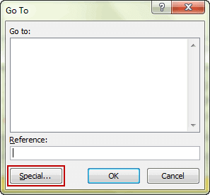
1. Press F5 and Go To dialog pops up. Click Special in dialog to open Go To Special dialog.

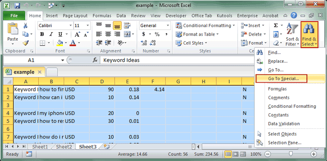
2. Click Home tab and Find & Select > Go To Special option in Editing group. Then Go To Special dialog appears.

Step 3: Select or check Blanks option in Go To Special dialog. And click OK.

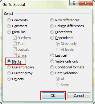
Then you would find in the data range you specify, all of blank cells are selected.

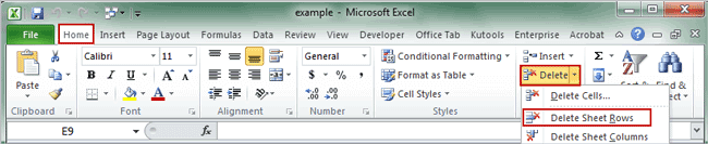
Step 4: Click Delete > Delete Sheet Rows/Delete Sheet Columns in Home tab and Cells group.

Then all the blank rows or columns will be deleted or removed in Excel.

Method 2: Eliminate blank rows by Excel filter functionality

Step 1: Select the range from which you need to remove the blank rows.

Step 2: Click Home > Sort & Filter > Filter in Editing group.

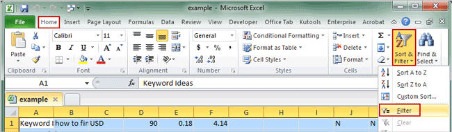
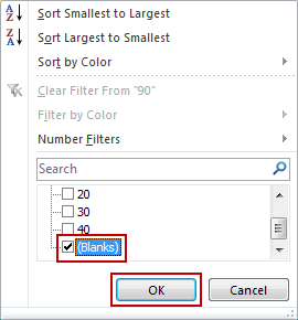
Step 3: Select a column and click the filter dropdown, uncheck the values excepting Blanks and click OK.

Step 4: With all the blank rows you select, click “Home > Delete > Delete Sheet Rows” to delete or remove all empty rows.

Related Articles:

• Remove and Bypass Excel Sheet Protection Password on Workbook
• How to Remove Restrict Editing in Excel 2007-2016 without Password
• How to Remove or Change Comment Author Name in Excel 2016/2013/2010
• 2 Options to Prevent Excel Sheets from Deletion

– How to Insert Cells and Shift Cells Down
– How to Delete Cells and Shift Cells Left
– How to Insert Cells and Shift Cells Right

When working with Excel, you may often need to delete cells. Please follow the steps below to delete cells and shift other cells up:

Step 1: Click the cell or cells where you want to delete;

Step 2: Right-click, and select «Delete» from the list in the dialog box.

Alternatively, please use the commands from the ribbonl

Step 1: Click the «Home» tab from the ribbon;

Step 2: Click «Delete» from the Cells area, and select «Delete Cells» from the drop-down list;

Step 3: In the «Delete» dialog box, click «Shift cells up«;

Step 4: Click «OK» at the bottom.