Relative path in excel

A path is a unique location for a file or a folder. There are broadly two types of paths, absolute path, and relative path. An absolute path gives the location of a file from its root folder, while a relative path gives the location of a file from its current folder. Power Query, by default, provides an absolute path, which could cause problems while sharing the files, so we have to reduce the absolute path to a relative path. In this article, we will learn how to convert an absolute path to a relative path, using a power query editor, and make our source files sharable.

Problem with Absolute Path

By default, our excel sheets have the location for absolute paths and not the relative paths. Due, to this file sharing, is a big and significant issue. For example, an analyst is analyzing data in its intelligence tools source via power query from your PC, the tools work well until the files are in your PC, but stop working as soon as they are imported into the third person PC, this happens because the absolute path in the third person computer might be different, and our power query files are still searching for the old absolute path provided in my computer. To resolve this issue, one needs to convert this absolute path to the relative path, so that the files can access irrespective of one’s PC.

Excel Functions Used in Converting Absolute Path to Relative Path

Before moving forward, we need to have a crisp knowledge of all the excel functions, that will be used to convert an Absolute path to a Relative path. There are broadly three functions used: =CELL(), =LEFT(), =FIND(), for creating the required formula:

Cell Function

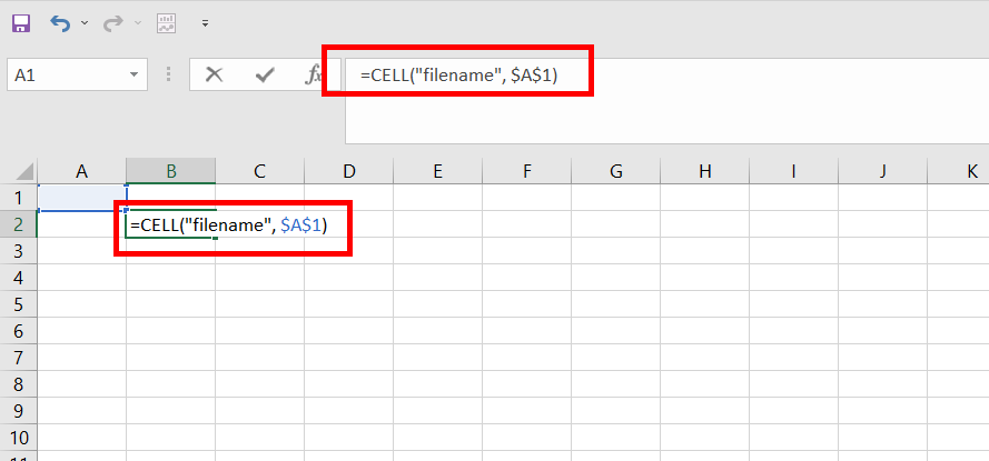
Syntax: =CELL(info_type, reference)

The cell function provides every information, you require, for a cell. One can get the value of a cell, its row number, address, filepath, etc. This topic could be quite big itself, but for converting absolute path to relative path, we only need to know about how to get the file path of a cell. There are two arguments in cell functions:

Argument 1: Info_type is the first argument of cell function. The type of information you want to find for the specified cell. For example, “filepath”, provides the absolute path for the current cell.
Argument 2: For which cell, do you want to extract the information. The cell reference can be absolute or relative.

Note: The excel file should be saved in some folder, then only the absolute path would appear, otherwise it will show an empty string returned. This is one of the common errors that users face while working with the =CELL(info_type, reference) function.

For example, find the absolute path of the current opened excel file. Following are the steps:

Step 1: Type =CELL(“filename”, $A$1), in cell B2, where “filename” provides the absolute reference of the file, and $A$1 is the reference to cell A1.

Step 2: Press Enter. The absolute Path of the current excel file appears in cell B2 i.e. D:geeksforgeeksfolder1folder2[geeksample.xlsx]Sheet1.

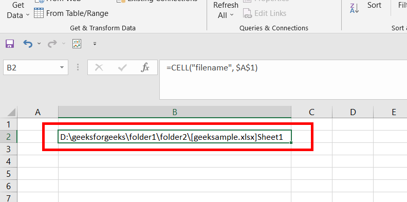
Step 3: The path before the bracket is the absolute path for that excel file. The text inside the square brackets is the name of the workbook, and at last, is the name of the worksheet.

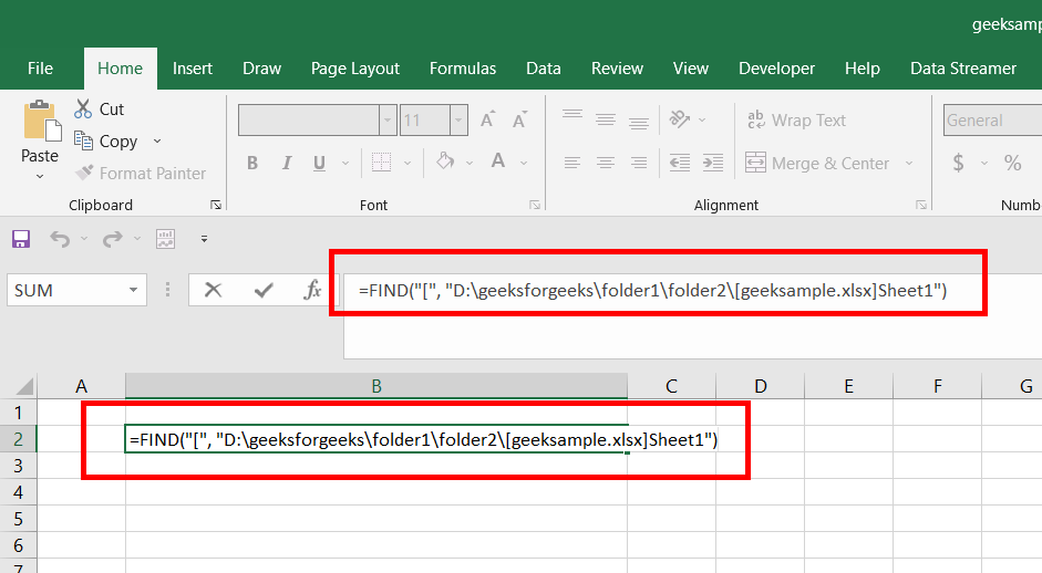
Find Function

Syntax: =FIND(find_text, within_text, [start_num])

The function finds the first starting index of the location of a finding text in the given string. The indexing is 1-based. For example, if you are given a string “geeksforgeeks”, and you want to find the position of “ks” in your given string, then the answer returned by the =FIND() function will be 4. There are three arguments in the find function, but for converting the absolute path to a relative path, we will require only the first two arguments.

Argument 1: Find_text is the first argument of the find function. The find_text is the string that needs to be found in the given string. The first occurrence of the find_text is printed using the =FIND() function.
Argument 2: Within_text is the second argument of the find function. The within_text is the original string in which find_text is searched.
Argument 3: This is an optional argument. It tells from which index you should start the search in the within_text.

For example, you recently found the absolute path for the current excel file, our task is to find the index of “[” (square bracket) in the given string i.e. “D:geeksforgeeksfolder1folder2[geeksample.xlsx]Sheet1”. Following are the steps:

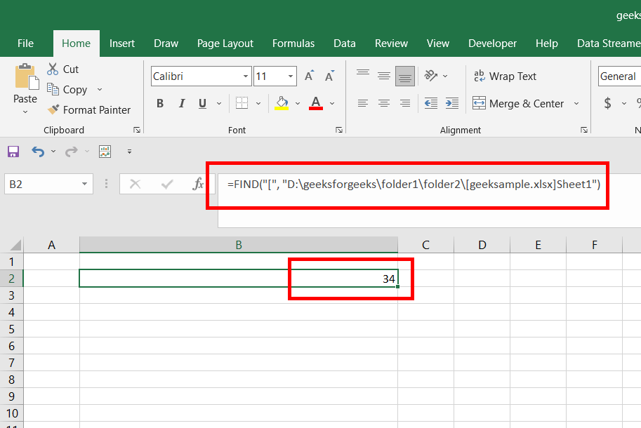
Step 1: Type =FIND(“[“, “D:geeksforgeeksfolder1folder2[geeksample.xlsx]Sheet1”), in the cell B2, where Argument1 is “[“ and Argument2 is “D:geeksforgeeksfolder1folder2[geeksample.xlsx]Sheet1”. Press Enter.

Step 2: We can see 34 appear in cell B2. This is because the “[“ appears at the 34th (1-based indexing) index in the original string.

Left Function

Syntax: =LEFT(text, [num_chars])

The function returns the prefix substring of a string, according to the user-specified number of characters. The indexing is 1-based. For example, if you are given a string “geeksforgeeks”, and you want to find the first four(4) characters in the given string, then we can use the =LEFT() function, to achieve this, the function will return a prefix substring “geek”. There are two arguments in the left function.

Argument 1: The first argument is the text string. The text string is the string for which the prefix substring has to be returned.
Argument 2: The second argument is num_chars. The num_chars is the number of characters you want from the starting of the text string.

For example, you recently found the absolute path of the current worksheet, and you also found the index of the square bracket “[” i.e. 34, our task is to find the prefix substring before the “[” (square bracket) which means the number of character to be 33. Following are the steps:

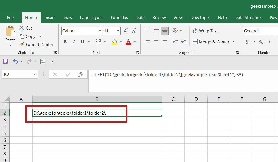
Step 1: Type =LEFT(“D:geeksforgeeksfolder1folder2[geeksample.xlsx]Sheet1”, 33), in the cell B2, where argument1 is the original string, for which prefix substring has to be returned, and the second argument is the number of characters for which this given string has to be returned.

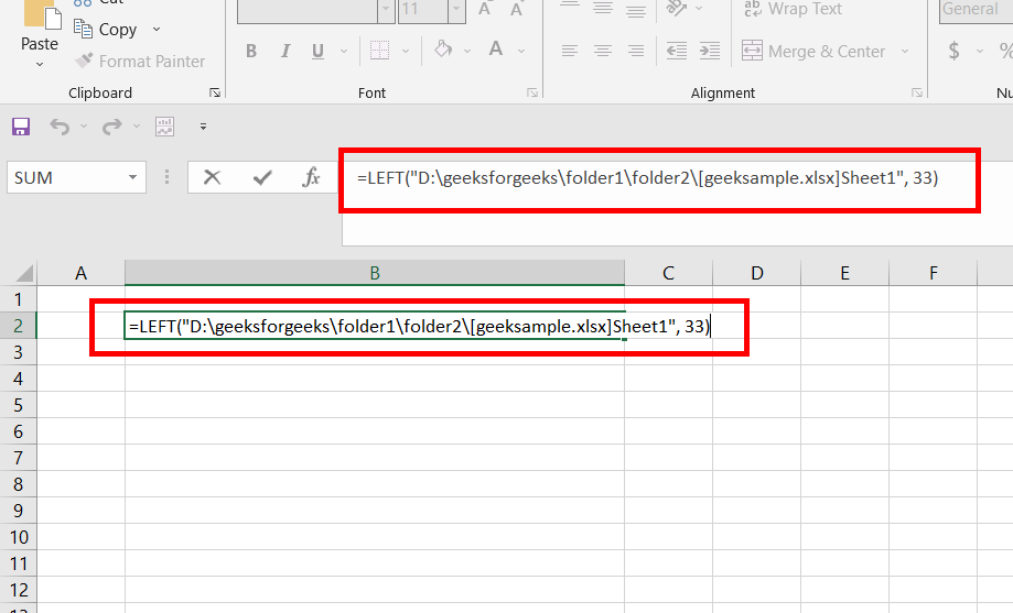
Step 2: Press Enter. All first 33 characters will appear in cell B2 i.e. “D:geeksforgeeksfolder1folder2”.

Converting Absolute Path to Relative Path in Power Query

Now, you know everything to convert an absolute path to a relative path, in a power query. We will take the same example and file location which we did, for understanding the functions. The absolute path for the current file is “D:geeksforgeeksfolder1folder2housing.csv”.This needs to be converted into the relative path. Following are the steps:

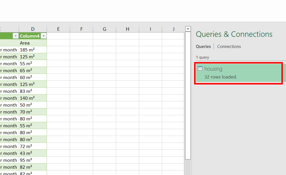
Step 1: As you are understanding an advanced topic of power query, so we will assume that you know how to get data from a CSV or xlsx file in power query. Imported a table, in the current sheet name “housing”, using Get Data.

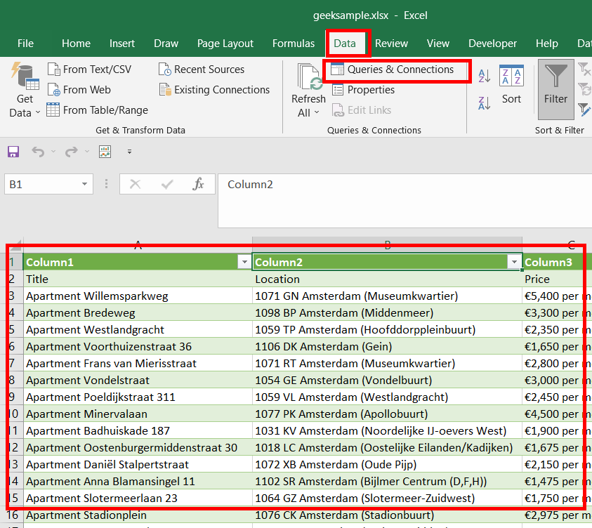
Step 2: Now, on the right side of your screen, you will have the housing data set, that you imported. Double-click on it and the power query editor will be launched. The main aim for step1 and step2 is to open our power query editor.

Step 3: The power Query editor is opened. In the Home tab, under the Query section, click on Advanced Editor.

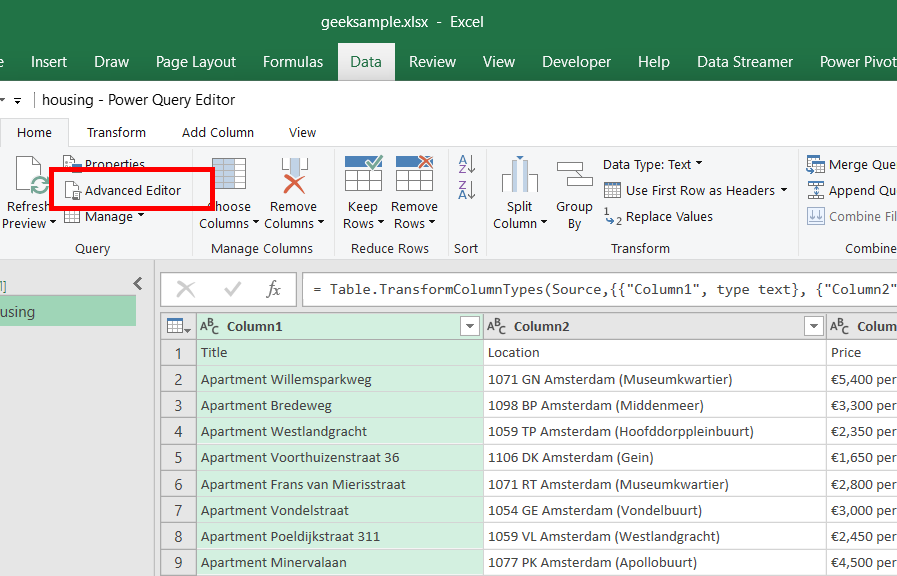
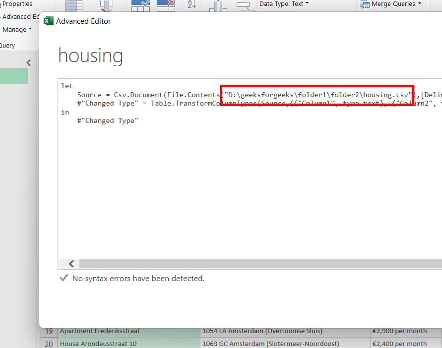
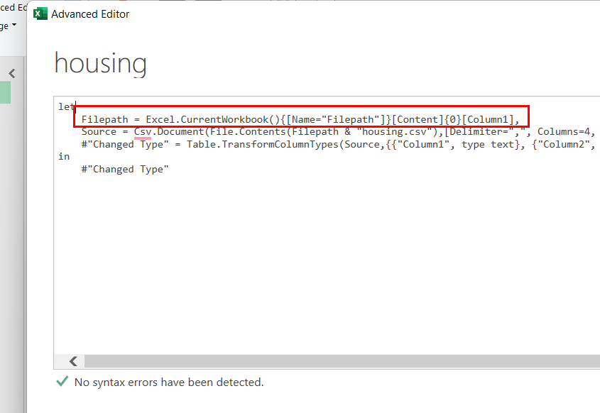
Step 4: The Advanced Editor is opened. You can observe that the M-code is written in the picture shown below, and the absolute path for the current CSV file is “D:geeksforgeeksfolder1folder2housing.csv”. Our task is to convert this absolute path into a relative path.

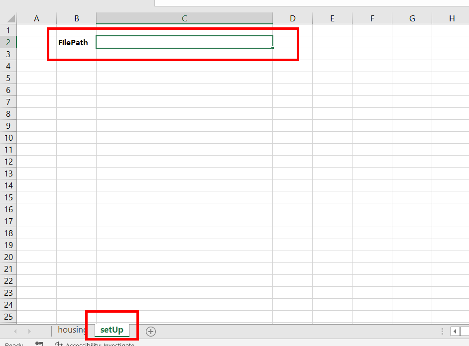
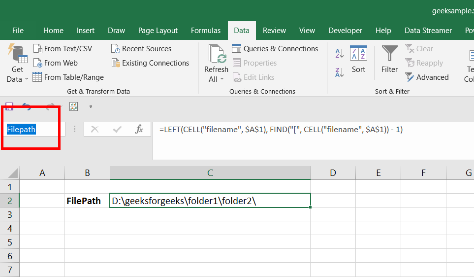
Step 5: Close all the windows, and return back to the “housing” worksheet. Now, create a new worksheet, named “setUp”. Cell B2 has the value FilePath.

Step 6: Now, comes the most important step. Now, if you have understood the examples provided while explaining the different functions like =CELL(), =FIND(), =LEFT(), then this will be a very easy step for you. The formula written is: =LEFT(CELL(“filename”, $A$1), FIND(“[“, CELL(“filename”, $A$1)) – 1). The formula simply extracts the text written before the square bracket “[“, in the absolute path, i.e. from “D:geeksforgeeksfolder1folder2[geeksample.xlsx]setUp” to “D:geeksforgeeksfolder1folder2” .

Step 7: Press Enter. “D:geeksforgeeksfolder1folder2” appears in the cell C2.

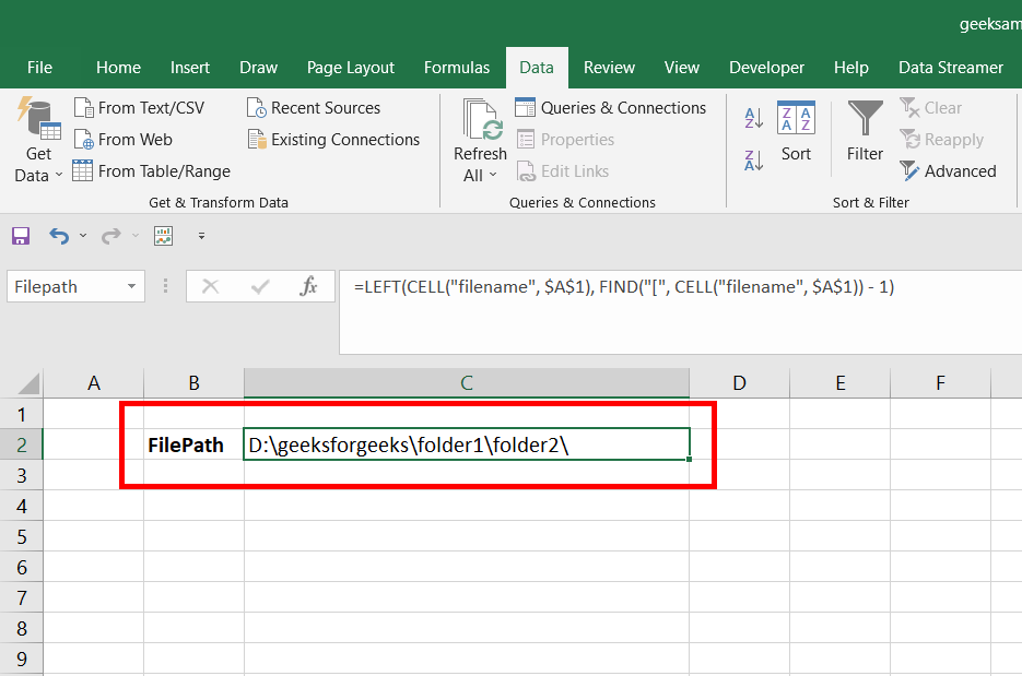
Step 8: Change the name of the cell, C3 to Filepath.

Step 9: Now, repeat steps 1, 2, and 3. This will open our advance editor again. Now, add this single line of M-code in your advanced editor, “Filepath = Excel.CurrentWorkbook(){[Name=”Filepath”]}[Content]{0}[Column1],”. This code simply stores the reference of the cell C3(Filepath) in the variable “Filepath”.

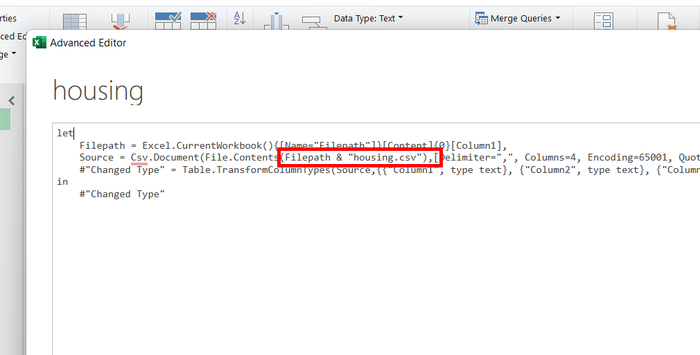
Step 10: Now, come to the second line of M-code, where some File content is stored in the variable “Source”. Inside the File.Contents function, change “D:geeksforgeeksfolder1folder2housing.csv” to ” Filepath & “housing.csv” “. Close all the windows, and return back to the “housing” worksheet, this converts your absolute path to the relative path of the current added data in your worksheet.

Источник

Содержание

Description of workbook link management and storage in Excel
Quak Quaks of the Ugly Duckling
How i learned to stop worrying and love the blog
Relative Paths in Excel Power Query instead of Absolute Paths
Explanation and usage:
Final remarks:
Work with links in Excel

Description of workbook link management and storage in Excel

In Microsoft Excel, you can link a cell in a workbook to another workbook using a formula that references the external workbook. This is called a workbook link. When this workbook link is created, it may use a relative path, which can enable you to move the workbooks without breaking the link. This article discusses how workbook links are stored by Excel under different circumstances and can help when you are trying to fix a broken link.

When Excel opens a destination workbook that contains workbook links, it dynamically combines the portions of the workbook links stored in the workbook with the necessary portions of the current path of the source workbook to create an absolute path.

It is also important to note that what appears in the formula bar is not necessarily what is stored. For example, if the source workbook is closed, you see a full path to the file, although only the file name may be stored.

Workbooks links to source workbooks are created in a relative manner whenever possible. This means that the full path to the source workbook is not recorded, but rather the portion of the path as it relates to the destination workbook. With this method, you can move the workbooks without breaking the links between them. The workbook links remain intact, however, only if the workbooks remain in the same location relative to each other. For example, if the destination workbook is C:MydirDestination.xlsx and the source workbook is C:MydirFilesSource.xlsx, you can move the files to the D drive as long as the source workbook is still located in a subfolder called «Files».

Relative links may cause problems if you move the destination workbook to different computers and the source workbook is in a central location.

The way workbook links are storied varies in the following ways:

Storage type 1: Same drive with the same folder or child folder

The source workbook is either in the same folder or a child folder as the destination workbook. In this case, we store the relative file path, for example, subfolder/source.xlsx and destination.xlsx.

This type works best for cloud-based workbooks and when both workbooks are moved.

Storage type 2: Same drive but with different sibling folders

The source and destination workbooks are on the same drive, but in different sibling folders. In this case, we store a server-relative path, for example, /root/parent/sibling1/source.xlsx and /root/parent/sibling2/destination.xlsx.

This type works best if the destination workbook is moved within the same drive, but the source workbook stays in the same location.

Storage type 3: Different drives

The source workbook is on a different drive from the destination workbook. For example, the destination workbook folder is on the C drive and the source workbook folder is on the H drive. In this case, we store the absolute path, for example, H:foldersource.xlsx or https://tenant.sharepoint.com/teams/site/folder/source.xlsx.

This type works best if the destination workbook is moved, but the source workbook stays in the same location. This assumes that the destination workbook can still access the source workbook.

If the source workbook is located in the XLStart, Alternate Startup File Location, or Library folder, a property is written to indicate one of these folders, and only the file name is stored.

Excel recognizes two default XLStart folders from which to automatically open files on startup. The two folders are as follows:

The XLStart folder that is in the user’s profile is the XLStart folder that is stored as a property for the workbook link. If you use the XLStart folder that is in the Office installation folder, that XLStart folder is treated like any other folder on the hard disk.

The Office folder name changes between versions of Office. For example, the Office folder name can be, Office14, Office15 or Office16, depending on the version of Office that you are running. This folder name change causes workbook links to be broken if you move to a computer that is running a different version of Excel than the version in which the link was established.

The XLStart folder that is in the Office installation folder, such as C:Program FilesMicrosoft Office XLStart

The XLStart folder that is in the user’s profile, such as C:Documents and Settings Application DataMicrosoftExcelXLStart

When a source workbook is linked, the workbook link is established based on the way that the source workbook was opened. If the workbook was opened over a mapped drive, the workbook link is created by using a mapped drive. The workbook link remains that way regardless of how the source workbook is opened in the future. If the source workbook is opened by a UNC path, the workbook link does not revert to a mapped drive, even if a matching drive is available. If you have both UNC and mapped drive workbook links in the same file, and the source workbooks are open at the same time as the destination workbook, only those links that match the way the source workbook was opened will react as hyperlink. Specifically, if you open the source workbook through a mapped drive and change the values in the source workbook, only those links created to the mapped drive will update immediately.

Also, the workbook link displayed in Excel may appear differently depending on how the workbook was opened. The workbook link may appear to match either the root UNC share or the root drive letter that was used to open the file.

There are several circumstances in which workbook links between workbooks can be inadvertently made to point to erroneous locations. The following are two of the most common scenarios.

You map a drive under the root of a share. For example, you map drive Z to \MyServerMyShareMyFolder1.

You create workbook links to a source workbook that is stored at the mapped location after you open the destination workbook through that mapped drive.

You open the destination workbook by a UNC path.

As a consequence, the workbook link will be broken.

If you close the destination workbook without saving it, the workbook links will not be changed. However, if you save the destination workbook before you close it, you will save the workbook links with the current broken path. The folders between the root of the share and the mapped folder will be left out of the path. In the example above, the link would change to \MyServerMyFolder1. In other words, the Share name is eliminated from the file path.

You map a drive under the root of a share. For example, you map drive Z to \MyServerMyShareMyFolder1.

You open the file by a UNC path, or a mapped drive mapped to a different folder on the share, such as \MyServerMyShareMyFolder2.

As a consequence, the workbook link will be broken.

Источник

Quak Quaks of the Ugly Duckling

How i learned to stop worrying and love the blog

Relative Paths in Excel Power Query instead of Absolute Paths

For the last few months, I have been spending a considerable amount of my time and attention in Power Query Editor in MS Excel.

I had 27 pre-formatted Excel workbooks containing a large amount of data. I needed to pull all data from 27 workbooks and aggregate them in another workbook, and calculate something based on the aggregated value. It worked fine.

I kept all the files in the same folder, zipped it, and extracted somewhere else to test. However some error occurred. After some hair-pulling and nail-biting, I realized the error is due to the absolute path being stored in the power query editor.

Hence, I came across the following solution to tell MS Power Query editor that please use relative paths instead of absolute paths.

Explanation and usage:

The following code returns the current path of the file.

So, paste it in any cell and click Formulas>Define Name, and name it as FilePath

The default version of the query looks like:

If we look carefully we would notice that the Source variable has the absolute file path in it. That is why if you move the files to a new location, the query will not work, because the absolute file path has been changed.

We are interested to change the value of the Source variable, so that it automatically gets the relative file path, instead absolute path.

To do th at, add the FilePath variable and modify the Source variable query as follows:

For my case, all the files were in a C:UsersBasaDesktopOBE Test v.0.3 folder. One aggregator file and 27 other source files.

I named the aggregator file as POC.xlsx, located in C:UsersBasaDesktopOBE Test v.0.3

I opened the POC.xlsx file and in a random cell Data!C6 pasted the following code.

C:UsersBasaDesktopOBE Test v.03

I named it as FilePath from the Formulas>Define Name

Therefore, the FilePath name will return the location of the aggregator file (POC.xlsx). I opened the POC.xlsx file, and clicked on Data>Get Data>From File>From Folder and browsed to the current location of the file, and clicked OK.

The list of all the files was shown, I clicked on Combine and Transform Data…

If you do not need to combine data from all the files, then click on Transform instead.

I needed to combine the data, so excel wanted me to select the sample file, following which it will combine the data. I selected the first file, since all the files were in the same structure.

After that the list of files will be shown in the Power Query Editor. Then click on Advanced Editor in the Home menu. Now is the time to use our FilePath name in the FilePath variable and modify the Source variable in the Power Query’s Advanced Editor.

Remember: there should not be any comma at the last line before in .

I modified the query as follows.

After you are done, click Done, and the data will be previewed. Design your query, and click close and load, or do what you need to do.

After writing this article, I think that there might be a confusion related to the FilePath variable/name. In the following query, the first FilePath is a variable, and the second FilePath is a name that we defined earlier from Data!C6 (i.e., the cell C6 of the sheet named Data).

To make it clearer, let me show an example. Say, you have defined the name of cell Data!C6 as Location ,

Then the query should look like as follows:

Источник

Work with links in Excel

For quick access to related information in another file or on a web page, you can insert a hyperlink in a worksheet cell. You can also insert links in specific chart elements.

Note: Most of the screen shots in this article were taken in Excel 2016. If you have a different version your view might be slightly different, but unless otherwise noted, the functionality is the same.

On a worksheet, click the cell where you want to create a link.

You can also select an object, such as a picture or an element in a chart, that you want to use to represent the link.

On the Insert tab, in the Links group, click Link .

You can also right-click the cell or graphic and then click Link on the shortcut menu, or you can press Ctrl+K.

Under Link to, click Create New Document.

In the Name of new document box, type a name for the new file.

Tip: To specify a location other than the one shown under Full path, you can type the new location preceding the name in the Name of new document box, or you can click Change to select the location that you want and then click OK.

Under When to edit, click Edit the new document later or Edit the new document now to specify when you want to open the new file for editing.

In the Text to display box, type the text that you want to use to represent the link.

To display helpful information when you rest the pointer on the link, click ScreenTip, type the text that you want in the ScreenTip text box, and then click OK.

On a worksheet, click the cell where you want to create a link.

You can also select an object, such as a picture or an element in a chart, that you want to use to represent the link.

On the Insert tab, in the Links group, click Link .

You can also right-click the cell or object and then click Link on the shortcut menu, or you can press Ctrl+K.

Under Link to, click Existing File or Web Page.

Do one of the following:

To select a file, click Current Folder, and then click the file that you want to link to.

You can change the current folder by selecting a different folder in the Look in list.

To select a web page, click Browsed Pages and then click the web page that you want to link to.

To select a file that you recently used, click Recent Files, and then click the file that you want to link to.

To enter the name and location of a known file or web page that you want to link to, type that information in the Address box.

To locate a web page, click Browse the Web , open the web page that you want to link to, and then switch back to Excel without closing your browser.

If you want to create a link to a specific location in the file or on the web page, click Bookmark, and then double-click the bookmark that you want.

Note: The file or web page that you are linking to must have a bookmark.

In the Text to display box, type the text that you want to use to represent the link.

To display helpful information when you rest the pointer on the link, click ScreenTip, type the text that you want in the ScreenTip text box, and then click OK.

To link to a location in the current workbook or another workbook, you can either define a name for the destination cells or use a cell reference.

To use a name, you must name the destination cells in the destination workbook.

How to name a cell or a range of cells

Select the cell, range of cells, or nonadjacent selections that you want to name.

Click the Name box at the left end of the formula bar .

Name box

In the Name box, type the name for the cells, and then press Enter.

Note: Names can’t contain spaces and must begin with a letter.

On a worksheet of the source workbook, click the cell where you want to create a link.

You can also select an object, such as a picture or an element in a chart, that you want to use to represent the link.

On the Insert tab, in the Links group, click Link .

You can also right-click the cell or object and then click Link on the shortcut menu, or you can press Ctrl+K.

Under Link to, do one of the following:

To link to a location in your current workbook, click Place in This Document.

To link to a location in another workbook, click Existing File or Web Page, locate and select the workbook that you want to link to, and then click Bookmark.

Do one of the following:

In the Or select a place in this document box, under Cell Reference, click the worksheet that you want to link to, type the cell reference in the Type in the cell reference box, and then click OK.

In the list under Defined Names, click the name that represents the cells that you want to link to, and then click OK.

In the Text to display box, type the text that you want to use to represent the link.

To display helpful information when you rest the pointer on the link, click ScreenTip, type the text that you want in the ScreenTip text box, and then click OK.

You can use the HYPERLINK function to create a link that opens a document that is stored on a network server, an intranet, or the Internet. When you click the cell that contains the HYPERLINK function, Excel opens the file that is stored at the location of the link.

Link_location is the path and file name to the document to be opened as text. Link_location can refer to a place in a document — such as a specific cell or named range in an Excel worksheet or workbook, or to a bookmark in a Microsoft Word document. The path can be to a file stored on a hard disk drive, or the path can be a universal naming convention (UNC) path on a server (in Microsoft Excel for Windows) or a Uniform Resource Locator (URL) path on the Internet or an intranet.

Link_location can be a text string enclosed in quotation marks or a cell that contains the link as a text string.

If the jump specified in link_location does not exist or can’t be navigated, an error appears when you click the cell.

Friendly_name is the jump text or numeric value that is displayed in the cell. Friendly_name is displayed in blue and is underlined. If friendly_name is omitted, the cell displays the link_location as the jump text.

Friendly_name can be a value, a text string, a name, or a cell that contains the jump text or value.

If friendly_name returns an error value (for example, #VALUE!), the cell displays the error instead of the jump text.

The following example opens a worksheet named Budget Report.xls that is stored on the Internet at the location named example.microsoft.com/report and displays the text «Click for report»:

=HYPERLINK(«http://example.microsoft.com/report/budget report.xls», «Click for report»)

The following example creates a link to cell F10 on the worksheet named Annual in the workbook Budget Report.xls, which is stored on the Internet at the location named example.microsoft.com/report . The cell on the worksheet that contains the link displays the contents of cell D1 as the jump text:

=HYPERLINK(«[http://example.microsoft.com/report/budget report.xls]Annual!F10», D1)

The following example creates a link to the range named DeptTotal on the worksheet named First Quarter in the workbook Budget Report.xls, which is stored on the Internet at the location named example.microsoft.com/report . The cell on the worksheet that contains the link displays the text «Click to see First Quarter Department Total»:

=HYPERLINK(«[http://example.microsoft.com/report/budget report.xls]First Quarter!DeptTotal», «Click to see First Quarter Department Total»)

To create a link to a specific location in a Microsoft Word document, you must use a bookmark to define the location you want to jump to in the document. The following example creates a link to the bookmark named QrtlyProfits in the document named Annual Report.doc located at example.microsoft.com :

=HYPERLINK(«[http://example.microsoft.com/Annual Report.doc]QrtlyProfits», «Quarterly Profit Report»)

In Excel for Windows, the following example displays the contents of cell D5 as the jump text in the cell and opens the file named 1stqtr.xls, which is stored on the server named FINANCE in the Statements share. This example uses a UNC path:

The following example opens the file 1stqtr.xls in Excel for Windows that is stored in a directory named Finance on drive D, and displays the numeric value stored in cell H10:

In Excel for Windows, the following example creates a link to the area named Totals in another (external) workbook, Mybook.xls:

In Microsoft Excel for the Macintosh, the following example displays «Click here» in the cell and opens the file named First Quarter that is stored in a folder named Budget Reports on the hard drive named Macintosh HD:

=HYPERLINK(«Macintosh HD:Budget Reports:First Quarter», «Click here»)

You can create links within a worksheet to jump from one cell to another cell. For example, if the active worksheet is the sheet named June in the workbook named Budget, the following formula creates a link to cell E56. The link text itself is the value in cell E56.

To jump to a different sheet in the same workbook, change the name of the sheet in the link. In the previous example, to create a link to cell E56 on the September sheet, change the word «June» to «September.»

When you click a link to an email address, your email program automatically starts and creates an email message with the correct address in the To box, provided that you have an email program installed.

On a worksheet, click the cell where you want to create a link.

You can also select an object, such as a picture or an element in a chart, that you want to use to represent the link.

On the Insert tab, in the Links group, click Link .

You can also right-click the cell or object and then click Link on the shortcut menu, or you can press Ctrl+K.

Under Link to, click E-mail Address.

In the E-mail address box, type the email address that you want.

In the Subject box, type the subject of the email message.

Note: Some web browsers and email programs may not recognize the subject line.

In the Text to display box, type the text that you want to use to represent the link.

To display helpful information when you rest the pointer on the link, click ScreenTip, type the text that you want in the ScreenTip text box, and then click OK.

You can also create a link to an email address in a cell by typing the address directly in the cell. For example, a link is created automatically when you type an email address, such as someone@example.com.

You can insert one or more external reference (also called links) from a workbook to another workbook that is located on your intranet or on the Internet. The workbook must not be saved as an HTML file.

Open the source workbook and select the cell or cell range that you want to copy.

On the Home tab, in the Clipboard group, click Copy.

Switch to the worksheet that you want to place the information in, and then click the cell where you want the information to appear.

On the Home tab, in the Clipboard group, click Paste Special.

Click Paste Link.

Excel creates an external reference link for the cell or each cell in the cell range.

Note: You may find it more convenient to create an external reference link without opening the workbook on the web. For each cell in the destination workbook where you want the external reference link, click the cell, and then type an equal sign (=), the URL address, and the location in the workbook. For example:

To select a hyperlink without activating the link to its destination, do one of the following:

Click the cell that contains the link, hold the mouse button until the pointer becomes a cross , and then release the mouse button.

Use the arrow keys to select the cell that contains the link.

If the link is represented by a graphic, hold down Ctrl, and then click the graphic.

You can change an existing link in your workbook by changing its destination, its appearance, or the text or graphic that is used to represent it.

Change the destination of a link

Select the cell or graphic that contains the link that you want to change.

Tip: To select a cell that contains a link without going to the link destination, click the cell and hold the mouse button until the pointer becomes a cross , and then release the mouse button. You can also use the arrow keys to select the cell. To select a graphic, hold down Ctrl and click the graphic.

On the Insert tab, in the Links group, click Link.

You can also right-click the cell or graphic and then click Edit Link on the shortcut menu, or you can press Ctrl+K.

In the Edit Hyperlink dialog box, make the changes that you want.

Note: If the link was created by using the HYPERLINK worksheet function, you must edit the formula to change the destination. Select the cell that contains the link, and then click the formula bar to edit the formula.

You can change the appearance of all link text in the current workbook by changing the cell style for links.

On the Home tab, in the Styles group, click Cell Styles.

Under Data and Model, do the following:

To change the appearance of links that have not been clicked to go to their destinations, right-click Link, and then click Modify.

To change the appearance of links that have been clicked to go to their destinations, right-click Followed Link, and then click Modify.

Note: The Link cell style is available only when the workbook contains a link. The Followed Link cell style is available only when the workbook contains a link that has been clicked.

In the Style dialog box, click Format.

On the Font tab and Fill tab, select the formatting options that you want, and then click OK.

The options that you select in the Format Cells dialog box appear as selected under Style includes in the Style dialog box. You can clear the check boxes for any options that you don’t want to apply.

Changes that you make to the Link and Followed Link cell styles apply to all links in the current workbook. You can’t change the appearance of individual links.

Select the cell or graphic that contains the link that you want to change.

Do one or more of the following:

To change the link text, click in the formula bar, and then edit the text.

To change the format of a graphic, right-click it, and then click the option that you need to change its format.

To change text in a graphic, double-click the selected graphic, and then make the changes that you want.

To change the graphic that represents the link, insert a new graphic, make it a link with the same destination, and then delete the old graphic and link.

Right-click the hyperlink that you want to copy or move, and then click Copy or Cut on the shortcut menu.

Right-click the cell that you want to copy or move the link to, and then click Paste on the shortcut menu.

By default, unspecified paths to hyperlink destination files are relative to the location of the active workbook. Use this procedure when you want to set a different default path. Each time that you create a link to a file in that location, you only have to specify the file name, not the path, in the Insert Hyperlink dialog box.

Follow one of the steps depending on the Excel version you are using:

In Excel 2016, Excel 2013, and Excel 2010:

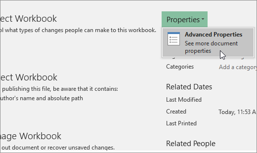
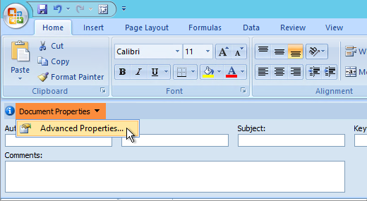
Click the File tab.

Click Properties, and then select Advanced Properties.

In the Summary tab, in the Hyperlink base text box, type the path that you want to use.

Note: You can override the link base address by using the full, or absolute, address for the link in the Insert Hyperlink dialog box.

Click the Microsoft Office Button , click Prepare, and then click Properties.

In the Document Information Panel, click Properties, and then click Advanced Properties.

Click the Summary tab.

In the Hyperlink base box, type the path that you want to use.

Note: You can override the link base address by using the full, or absolute, address for the link in the Insert Hyperlink dialog box.

To delete a link, do one of the following:

To delete a link and the text that represents it, right-click the cell that contains the link, and then click Clear Contents on the shortcut menu.

To delete a link and the graphic that represents it, hold down Ctrl and click the graphic, and then press Delete.

To turn off a single link, right-click the link, and then click Remove Link on the shortcut menu.

To turn off several links at once, do the following:

In a blank cell, type the number 1.

Right-click the cell, and then click Copy on the shortcut menu.

Hold down Ctrl and select each link that you want to turn off.

Tip: To select a cell that has a link in it without going to the link destination, click the cell and hold the mouse button until the pointer becomes a cross , and then release the mouse button.

On the Home tab, in the Clipboard group, click the arrow below Paste, and then click Paste Special.

Under Operation, click Multiply, and then click OK.

On the Home tab, in the Styles group, click Cell Styles.

Under Good, Bad, and Neutral, select Normal.

A link opens another page or file when you click it. The destination is frequently another web page, but it can also be a picture, or an email address, or a program. The link itself can be text or a picture.

When a site user clicks the link, the destination is shown in a Web browser, opened, or run, depending on the type of destination. For example, a link to a page shows the page in the web browser, and a link to an AVI file opens the file in a media player.

How links are used

You can use links to do the following:

Navigate to a file or web page on a network, intranet, or Internet

Navigate to a file or web page that you plan to create in the future

Send an email message

Start a file transfer, such as downloading or an FTP process

When you point to text or a picture that contains a link, the pointer becomes a hand , indicating that the text or picture is something that you can click.

What a URL is and how it works

When you create a link, its destination is encoded as a Uniform Resource Locator (URL), such as:

A URL contains a protocol, such as HTTP, FTP, or FILE, a Web server or network location, and a path and file name. The following illustration defines the parts of the URL:

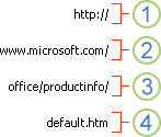
1. Protocol used (http, ftp, file)

2. Web server or network location

Absolute and relative links

An absolute URL contains a full address, including the protocol, the Web server, and the path and file name.

A relative URL has one or more missing parts. The missing information is taken from the page that contains the URL. For example, if the protocol and web server are missing, the web browser uses the protocol and domain, such as .com, .org, or .edu, of the current page.

It is common for pages on the web to use relative URLs that contain only a partial path and file name. If the files are moved to another server, any links will continue to work as long as the relative positions of the pages remain unchanged. For example, a link on Products.htm points to a page named apple.htm in a folder named Food; if both pages are moved to a folder named Food on a different server, the URL in the link will still be correct.

In an Excel workbook, unspecified paths to link destination files are by default relative to the location of the active workbook. You can set a different base address to use by default so that each time that you create a link to a file in that location, you only have to specify the file name, not the path, in the Insert Hyperlink dialog box.

Источник

Office Products Excel for Microsoft 365 Excel 2019 Excel 2016 Excel 2013 Excel 2010 More…Less

Relative links may cause problems if you move the destination workbook to different computers and the source workbook is in a central location.

The way workbook links are storied varies in the following ways:

Storage type 1: Same drive with the same folder or child folder

The source workbook is either in the same folder or a child folder as the destination workbook. In this case, we store the relative file path, for example, subfolder/source.xlsx and destination.xlsx.

This type works best for cloud-based workbooks and when both workbooks are moved.

Storage type 2: Same drive but with different sibling folders

This type works best if the destination workbook is moved within the same drive, but the source workbook stays in the same location.

Storage type 3: Different drives

This type works best if the destination workbook is moved, but the source workbook stays in the same location. This assumes that the destination workbook can still access the source workbook.

If the source workbook is located in the XLStart, Alternate Startup File Location, or Library folder, a property is written to indicate one of these folders, and only the file name is stored.

Excel recognizes two default XLStart folders from which to automatically open files on startup. The two folders are as follows:

The XLStart folder that is in the user’s profile is the XLStart folder that is stored as a property for the workbook link. If you use the XLStart folder that is in the Office installation folder, that XLStart folder is treated like any other folder on the hard disk.

The Office folder name changes between versions of Office. For example, the Office folder name can be, Office14, Office15 or Office16, depending on the version of Office that you are running. This folder name change causes workbook links to be broken if you move to a computer that is running a different version of Excel than the version in which the link was established.

The XLStart folder that is in the Office installation folder, such as C:Program FilesMicrosoft Office<Office folder>XLStart
The XLStart folder that is in the user’s profile, such as C:Documents and Settings<username>Application DataMicrosoftExcelXLStart

There are several circumstances in which workbook links between workbooks can be inadvertently made to point to erroneous locations. The following are two of the most common scenarios.

Scenario 1

You map a drive under the root of a share. For example, you map drive Z to \MyServerMyShareMyFolder1.
You create workbook links to a source workbook that is stored at the mapped location after you open the destination workbook through that mapped drive.
You open the destination workbook by a UNC path.
As a consequence, the workbook link will be broken.

Scenario 2

You map a drive under the root of a share. For example, you map drive Z to \MyServerMyShareMyFolder1.
You open the file by a UNC path, or a mapped drive mapped to a different folder on the share, such as \MyServerMyShareMyFolder2.
As a consequence, the workbook link will be broken.

How do you reference a relative path in Excel?

@James ='[ComponentsC. xlsx]Sheet1′! A1 used to work fine, but now Excel automatically changes the link to full path :-(.

How do you create a relative link in Excel?

Figure 1.

Choose Properties from the File menu. Excel displays the Properties dialog box.
Make sure the Summary tab is selected. (See Figure 2.)
In the Hyperlink Base box, indicate the first part of any URL specified using relative references.
Click on OK when finished.

How do I link to a folder path in Excel?

Below are the steps to create a hyperlink to a folder:

Copy the folder address for which you want to create the hyperlink.
Select the cell in which you want the hyperlink.
Click the Insert tab.
Click the links button.
In the Insert Hyperlink dialog box, paste folder address.
Click OK.

What is a relative path in Excel?

In Microsoft Excel, you can link a cell in a workbook to another workbook using a formula that references the external workbook. When this link is created, it may use a relative path. With a relative link, you can move the workbooks without breaking the link.

How do I import file names into Excel?

How to import multiple file names into cells in Excel?

Launch a new worksheet that you want to import the file names.
Hold down the ALT + F11 keys to open the Microsoft Visual Basic for Applications window.
Click Insert > Module, and paste the following code in the Module Window.

Which is the best way to import data from a text file into Excel?

Steps to convert content from a TXT or CSV file into Excel

Open the Excel spreadsheet where you want to save the data and click the Data tab.
In the Get External Data group, click From Text.
Select the TXT or CSV file you want to convert and click Import.
Select “Delimited”.
Click Next.

How do I create URLs in Excel based on data in another cell?

Insert a Hyperlink

Select the cell where you want the hyperlink.
On the Excel Ribbon, click the Insert tab, and click the Hyperlink command. OR, right-click the cell, and click Link. OR, use the keyboard shortcut – Ctrl + K.

Can I hyperlink to a specific cell in Excel?

Answer: To create a hyperlink to another cell in your spreadsheet, right click on the cell where the hyperlink should go. Select Hyperlink from the popup menu. When the Insert Hyperlink window appears, click on the “Place In This Document” on the left. Enter the text to display.

What is an absolute path in Excel?

An absolute path defines the absolute location of the file within the file system. It is commonly used for resources that serve as data sources for the model (for example, text or Excel files) and are stored outside of the model folder (for example, on a file server or in a shared folder).

What is the fastest way to copy file names into Excel?

Let’s jump right into it.

Step 1: Open Excel. Open up excel and then navigate to the folder that contains the files.
Step 2: Navigate to Folder and Select All the Files.
Step 3: Hold Shift Key and Right Click.
Step 4: Click Copy as Path.
Step 5: Paste Filepaths in Excel.
Step 6: Use Replace Function in Excel.

Источник

So it is possible to have a relative path instead of an absolute path, so your data sources continue to work as long as you keep the data source files in the same location as the worksheet that uses them.

The Excel user interface does not seem to have any way for changing the path though.

But you can edit the XLSX in a different way than with the UI. If you rename your XLSX file to .zip, you can extract it «as-if» it is a zip file (actually the excel workbook is a compressed file). Then in the extracted zip file, open the xl directory, and therein the file «connections.xml»

There you’ll find the «sourceFile», you can change this and have it refer to the file name only.

Then, move the «connections.xml» back into the «zipped» excel file, and rename it back to XLSX.

Note just zipping the directory back and renaming it to XLSX won’t do, because any zip command may use a variation of compression algorithms and options that won’t always be compatible with microsoft excel…

So best is to move the «connections.xml» back into the already existing zip file (or even better, edit the file directly in the zip file, if your zip file handler allows it).

The ExcelFile.xlsxxlconnections.xml file will look something like this:

<?xml version="1.0" encoding="UTF-8" standalone="yes"?>
<connections xmlns="http://schemas.openxmlformats.org/spreadsheetml/2006/main" xmlns:mc="http://schemas.openxmlformats.org/markup-compatibility/2006" mc:Ignorable="xr16" xmlns:xr16="http://schemas.microsoft.com/office/spreadsheetml/2017/revision16"><connection id="1" xr16:uid="{F9606253-9C57-4B65-839A-8DEF5AAEA9F7}" keepAlive="1" name="ThisWorkbookDataModel" description="Data Model" type="5" refreshedVersion="6" minRefreshableVersion="5" background="1"><dbPr connection="Data Model Connection" command="Model" commandType="1"/><olapPr sendLocale="1" rowDrillCount="1000"/><extLst><ext uri="{DE250136-89BD-433C-8126-D09CA5730AF9}" xmlns:x15="http://schemas.microsoft.com/office/spreadsheetml/2010/11/main"><x15:connection id="" model="1"/></ext></extLst></connection><connection id="2" xr16:uid="{7FE915B8-2095-40EC-B6DC-A589A5A2D08D}" name="TimeTrackingUserEntryLog" type="103" refreshedVersion="6" minRefreshableVersion="5" refreshOnLoad="1" saveData="1"><extLst><ext uri="{DE250136-89BD-433C-8126-D09CA5730AF9}" xmlns:x15="http://schemas.microsoft.com/office/spreadsheetml/2010/11/main"><x15:connection id="TimeTrackingUserEntryLog" autoDelete="1"><x15:textPr prompt="0" sourceFile="C:DropboxWonderfulLifeorLiveTimeTrackingUserEntryLog.csv" tab="0" comma="1"><textFields count="5"><textField type="YMD"/><textField/><textField type="text"/><textField type="text"/><textField type="text"/></textFields></x15:textPr><x15:modelTextPr headers="1"/></x15:connection></ext></extLst></connection></connections>

where the C:Dropbox etc is the path to my datasource which happens to be a csv file.

You can remove the entire path and just leave «datasourcefilename.csv» there.

Hope that helps! ^^

Источник

For the last few months, I have been spending a considerable amount of my time and attention in Power Query Editor in MS Excel.

Hence, I came across the following solution to tell MS Power Query editor that please use relative paths instead of absolute paths.

https://techcommunity.microsoft.com/t5/excel/power-query-source-from-relative-paths/m-p/206150

Credit goes to Sergei Baklan

Explanation and usage:

The following code returns the current path of the file.

=LEFT(CELL("filename",$A$1),FIND("[",CELL("filename",$A$1),1)-1)

So, paste it in any cell and click Formulas>Define Name, and name it as FilePath

The default version of the query looks like:

let
Source = Folder.Files("C:UsersBasaDesktopOBE Test v.03"),
....some more code...
in
#"Changed Type"

We are interested to change the value of the Source variable, so that it automatically gets the relative file path, instead absolute path.

To do that, add the FilePath variable and modify the Source variable query as follows:

let
FilePath = Excel.CurrentWorkbook(){[Name="FilePath"]}[Content]{0}[Column1],
Source = Folder.Files(FilePath),
....some more code...
in
#"Changed Type"

For my case, all the files were in a C:UsersBasaDesktopOBE Test v.0.3 folder. One aggregator file and 27 other source files.

I named the aggregator file as POC.xlsx, located in C:UsersBasaDesktopOBE Test v.0.3

I opened the POC.xlsx file and in a random cell Data!C6 pasted the following code.

=LEFT(CELL("filename",$A$1),FIND("[",CELL("filename",$A$1),1)-1)

At it returned

C:UsersBasaDesktopOBE Test v.03

I named it as FilePath from the Formulas>Define Name

The list of all the files was shown, I clicked on Combine and Transform Data…

If you do not need to combine data from all the files, then click on Transform instead.

I needed to combine the data, so excel wanted me to select the sample file, following which it will combine the data. I selected the first file, since all the files were in the same structure.

Remember: there should not be any comma at the last line before in.

I modified the query as follows.

After you are done, click Done, and the data will be previewed. Design your query, and click close and load, or do what you need to do.

End.

Final remarks:

 FilePath = Excel.CurrentWorkbook(){[Name="FilePath"]}[Content]{0}[Column1],
 Source = Folder.Files(FilePath),

To make it clearer, let me show an example. Say, you have defined the name of cell Data!C6 as Location,

Then the query should look like as follows:

FilePath = Excel.CurrentWorkbook(){[Name="Location"]}[Content]{0}[Column1],
Source = Folder.Files(FilePath),

Источник

Date yes Add (Subtract) Days to a Date Concatenate Dates Convert Date to Number Convert Date to Text Month Name to Number Create Date Range from Dates Day Number of Year Month Name from Date First Day of Month Add (Subtract) Weeks to a Date If Functions with Dates Max Date Number of Days Between Dates Number of Days in a Month Number of Weeks Between Dates Number of Years Between Dates Split Date & Time into Separate Cells Countdown Remaining Days Insert Dates Random Date Generator Using Dynamic Ranges — Year to Date Values Add (Subtract) Years to a Date Date Formula Examples Extract Day from Date Get Day Name from Date Count Days Left in Month / Year Count Workdays Left in Month / Year Get Last Day of Month Last Business Day of Month / Year Number of Work / Business Days in Month Weekday Abbreviations Auto Populate Dates Number of Months Between Dates Quarter from a Date Years of Service Change Date Format Compare Dates Time yes Add (Subtract) Hours to Time Add (Subtract) Minutes to Time Add (Subtract) Seconds to Time Add Up time (Total Time) Time Differences Change Time Format Convert Minutes to Hours Convert Time to Decimal Convert Time to Hours Convert Time to Minutes Convert Time to Seconds Military Time Round Time to Nearest 15 Minutes Overtime Calculator Number of Hours Between Times Convert Seconds to Minutes, Hours, or Time Count Hours Worked Time Differences Time Format — Show Minutes Seconds Text yes Add Commas to Cells Get First Word from Text Capitalize First Letter Clean & Format Phone #s Remove Extra Trailing / Leading Spaces Add Spaces to Cell Assign Number Value to Text Combine Cells with Comma Combine First and Last Names Convert Text String to Date Convert Text to Number Extract Text From Cell Get Last Word Remove Unwated Characters Extract Text Before or After Character How to Split Text String by Space, Comma, & More Remove Special Characters Remove First Characters from Left Substitute Multiple Values Switch First & Last Names w/ Commas Remove Specific Text from a Cell Extract Text Between Characters (Ex. Parenthesis) Add Leading Zeros to a Number Remove Line Breaks from Text Remove all Numbers from Text Reverse Text Remove Non-Numeric Characters Remove Last Character(s) From Right Separate First and Last Names Separate Text & Numbers Round yes Round Formulas Round Price to Nearest Dollar or Cent Round to Nearest 10, 100, or 1000 Round to Nearest 5 or .5 Round Percentages Round to Significant Figures Count yes Count Blank and Non-blank Cells Count Cells Between Two Numbers Count Cells not Equal to Count if Cells are in Range Count Times Word Appears in Cell Count Words in Cell Count Specific Characters in Column Count Total Number of Characters in Column Count Cells that Equal one of two Results Count Cells that do not Contain Count Cells that Contain Specific Text Count Unique Values in Range Countif — Multiple Criteria Count Total Number of Cells in Range Count Cells with Any Text Count Total Cells in a Table Lookup yes Two Dimensional VLOOKUP VLOOKUP Simple Example Vlookup — Multiple Matches Case Sensitive Lookup Case Sensitive VLOOKUP Sum if — VLOOKUP Case Sensitive Lookup Case Sensitive VLOOKUP Find Duplicates w/ VLOOKUP or MATCH INDEX MATCH MATCH Lookup — Return Cell Address (Not Value) Lookup Last Value in Column or Row Reverse VLOOKUP (Right to Left) Risk Score Bucket with VLOOKUP Sum with a VLOOKUP Function VLOOKUP & INDIRECT VLOOKUP Concatenate VLOOKUP Contains (Partial Match) 17 Reasons Why Your XLOOKUP is Not Working Double (Nested) XLOOKUP — Dynamic Columns IFERROR (& IFNA) XLOOKUP Lookup Min / Max Value Nested VLOOKUP Top 11 Alternatives to VLOOKUP (Updated 2022!) VLOOKUP – Dynamic Column Reference VLOOKUP – Fix #N/A Error VLOOKUP – Multiple Sheets at Once VLOOKUP & HLOOKUP Combined VLOOKUP & MATCH Combined VLOOKUP Between Worksheets or Spreadsheets VLOOKUP Duplicate Values VLOOKUP Letter Grades VLOOKUP Return Multiple Columns VLOOKUP Returns 0? Return Blank Instead VLOOKUP w/o #N/A Error XLOOKUP Multiple Sheets at Once XLOOKUP Between Worksheets or Spreadsheets XLOOKUP by Date XLOOKUP Duplicate Values XLOOKUP Multiple Criteria XLOOKUP Return Multiple Columns XLOOKUP Returns 0? Return Blank Instead XLOOKUP Text XLOOKUP with IF XLOOKUP With If Statement Misc. yes Sort Multiple Columns Use Cell Value in Formula Percentage Change Between Numbers Percentage Breakdown Rank Values Add Spaces to Cell CAGR Formula Average Time Decimal Part of Number Integer Part of a Number Compare Items in a List Dealing with NA() Errors Get Worksheet Name Wildcard Characters Hyperlink to Current Folder Compound Interest Formula Percentage Increase Create Random Groups Sort with the Small and Large Functions Non-volatile Function Alternatives Decrease a Number by a Percentage Calculate Percent Variance Profit Margin Calculator Convert Column Number to Letter Get Full Address of Named Range Insert File Name Insert Path Latitute / Longitude Functions Replace Negative Values Reverse List Range Convert State Name to Abbreviation Create Dynamic Hyperlinks Custom Sort List with Formula Data Validation — Custom Formulas Dynamic Sheet Reference (INDIRECT) Reference Cell in Another Sheet or Workbook Get Cell Value by Address Get Worksheet Name Increment Cell Reference List Sheet Names List Skipped Numbers in Sequence Return Address of Max Value in Range Search by Keywords Select Every Other (or Every nth) Row Basics yes Cell Reference Basics — A1, R1C1, 3d, etc. Add Up (Sum) Entire Column or Row Into to Dynamic Array Formulas Conversions yes Convert Time Zones Convert Celsius to Fahrenheit Convert Pounds to Kilograms Convert Time to Unix Time Convert Feet to Meters Convert Centimeters to Inches Convert Kilometers to Miles Convert Inches to Feet Convert Date to Julian Format Convert Column Letter to Number Tests yes Test if a Range Contains any Text Test if any Cell in Range is Number Test if a Cell Contains a Specific Value Test if Cell Contains Any Number Test if Cell Contains Specific Number Test if Cell is Number or Text If yes Percentile If Subtotal If Sumproduct If Large If and Small If Median If Concatentate If Max If Rank If TEXTJOIN If Sum yes Sum if — Begins With / Ends With Sum if — Month or Year to Date Sum if — By Year Sum if — Blank / Non-Blank Sum if — Horizontal Sum Count / Sum If — Cell Color INDIRECT Sum Sum If — Across Multiple Sheets Sum If — By Month Sum If — Cells Not Equal To Sum If — Not Blank Sum if — Between Values Sum If — Week Number Sum Text Sum if — By Category or Group Sum if — Cell Contains Specific Text (Wildcards) Sum if — Date Rnage Sum if — Dates Equal Sum if — Day of Week Sum if — Greater Than Sum if — Less Than Average yes Average Non-Zero Values Average If — Not Blank Average — Ignore 0 Average — Ignore Errors Math yes Multiplication Table Cube Roots nth Roots Square Numbers Square Roots Calculations yes Calculate a Ratio Calculate Age KILLLLLLL Calculate Loan Payments GPA Formula Calculate VAT Tax How to Grade Formulas Find yes Find a Number in a Column / Workbook Find Most Frequent Numbers Find Smallest n Values Find nth Occurance of Character in Text Find and Extract Number from String Find Earliest or Latest Date Based on Criteria Find First Cell with Any Value Find Last Row Find Last Row with Data Find Missing Values Find Largest n Values Most Frequent Number Conditional Formatting yes Conditional Format — Dates & Times Conditional Format — Highlight Blank Cells New Functions XLOOKUP Replaces VLOOKUP, HLOOKUP, and INDEX / MATCH Logical yes AND Checks whether all conditions are met. TRUE/FALSE IF If condition is met, do something, if not, do something else. IFERROR If result is an error then do something else. NOT Changes TRUE to FALSE and FALSE to TRUE. OR Checks whether any conditions are met. TRUE/FALSE XOR Checks whether one and only one condition is met. TRUE/FALSE Lookup & Reference yes FALSE The logical value: FALSE. TRUE The logical value: TRUE. ADDRESS Returns a cell address as text. AREAS Returns the number of areas in a reference. CHOOSE Chooses a value from a list based on it’s position number. COLUMN Returns the column number of a cell reference. COLUMNS Returns the number of columns in an array. HLOOKUP Lookup a value in the first row and return a value. HYPERLINK Creates a clickable link. INDEX Returns a value based on it’s column and row numbers. INDIRECT Creates a cell reference from text. LOOKUP Looks up values either horizontally or vertically. MATCH Searches for a value in a list and returns its position. OFFSET Creates a reference offset from a starting point. ROW Returns the row number of a cell reference. ROWS Returns the number of rows in an array. TRANSPOSE Flips the oriention of a range of cells. VLOOKUP Lookup a value in the first column and return a value. Date & Time yes DATE Returns a date from year, month, and day. DATEDIF Number of days, months or years between two dates. DATEVALUE Converts a date stored as text into a valid date DAY Returns the day as a number (1-31). DAYS Returns the number of days between two dates. DAYS360 Returns days between 2 dates in a 360 day year. EDATE Returns a date, n months away from a start date. EOMONTH Returns the last day of the month, n months away date. HOUR Returns the hour as a number (0-23). MINUTE Returns the minute as a number (0-59). MONTH Returns the month as a number (1-12). NETWORKDAYS Number of working days between 2 dates. NETWORKDAYS.INTL Working days between 2 dates, custom weekends. NOW Returns the current date and time. SECOND Returns the second as a number (0-59) TIME Returns the time from a hour, minute, and second. TIMEVALUE Converts a time stored as text into a valid time. TODAY Returns the current date. WEEKDAY Returns the day of the week as a number (1-7). WEEKNUM Returns the week number in a year (1-52). WORKDAY The date n working days from a date. WORKDAY.INTL The date n working days from a date, custom weekends. YEAR Returns the year. YEARFRAC Returns the fraction of a year between 2 dates. Engineering yes CONVERT Convert number from one unit to another. Financial yes FV Calculates the future value. PV Calculates the present value. NPER Calculates the total number of payment periods. PMT Calculates the payment amount. RATE Calculates the interest Rate. NPV Calculates the net present value. IRR The internal rate of return for a set of periodic CFs. XIRR The internal rate of return for a set of non-periodic CFs. PRICE Calculates the price of a bond. YIELD Calculates the bond yield. INTRATE The interest rate of a fully invested security. Information yes CELL Returns information about a cell. ERROR.TYPE Returns a value representing the cell error. ISBLANK Test if cell is blank. TRUE/FALSE ISERR Test if cell value is an error, ignores #N/A. TRUE/FALSE ISERROR Test if cell value is an error. TRUE/FALSE ISEVEN Test if cell value is even. TRUE/FALSE ISFORMULA Test if cell is a formula. TRUE/FALSE ISLOGICAL Test if cell is logical (TRUE or FALSE). TRUE/FALSE ISNA Test if cell value is #N/A. TRUE/FALSE ISNONTEXT Test if cell is not text (blank cells are not text). TRUE/FALSE ISNUMBER Test if cell is a number. TRUE/FALSE ISODD Test if cell value is odd. TRUE/FALSE ISREF Test if cell value is a reference. TRUE/FALSE ISTEXT Test if cell is text. TRUE/FALSE N Converts a value to a number. NA Returns the error: #N/A. TYPE Returns the type of value in a cell. Math yes ABS Calculates the absolute value of a number. AGGREGATE Define and perform calculations for a database or a list. CEILING Rounds a number up, to the nearest specified multiple. COS Returns the cosine of an angle. DEGREES Converts radians to degrees. DSUM Sums database records that meet certain criteria. EVEN Rounds to the nearest even integer. EXP Calculates the exponential value for a given number. FACT Returns the factorial. FLOOR Rounds a number down, to the nearest specified multiple. GCD Returns the greatest common divisor. INT Rounds a number down to the nearest integer. LCM Returns the least common multiple. LN Returns the natural logarithm of a number. LOG Returns the logarithm of a number to a specified base. LOG10 Returns the base-10 logarithm of a number. MOD Returns the remainder after dividing. MROUND Rounds a number to a specified multiple. ODD Rounds to the nearest odd integer. PI The value of PI. POWER Calculates a number raised to a power. PRODUCT Multiplies an array of numbers. QUOTIENT Returns the integer result of division. RADIANS Converts an angle into radians. RAND Calculates a random number between 0 and 1. RANDBETWEEN Calculates a random number between two numbers. ROUND Rounds a number to a specified number of digits. ROUNDDOWN Rounds a number down (towards zero). ROUNDUP Rounds a number up (away from zero). SIGN Returns the sign of a number. SIN Returns the sine of an angle. SQRT Calculates the square root of a number. SUBTOTAL Returns a summary statistic for a series of data. SUM Adds numbers together. SUMIF Sums numbers that meet a criteria. SUMIFS Sums numbers that meet multiple criteria. SUMPRODUCT Multiplies arrays of numbers and sums the resultant array. TAN Returns the tangent of an angle. TRUNC Truncates a number to a specific number of digits. Stats yes AVERAGE Averages numbers. AVERAGEA Averages numbers. Includes text & FALSE =0, TRUE =1. AVERAGEIF Averages numbers that meet a criteria. AVERAGEIFS Averages numbers that meet multiple criteria. CORREL Calculates the correlation of two series. COUNT Counts cells that contain a number. COUNTA Count cells that are non-blank. COUNTBLANK Counts cells that are blank. COUNTIF Counts cells that meet a criteria. COUNTIFS Counts cells that meet multiple criteria. FORECAST Predict future y-values from linear trend line. FREQUENCY Counts values that fall within specified ranges. GROWTH Calculates Y values based on exponential growth. INTERCEPT Calculates the Y intercept for a best-fit line. LARGE Returns the kth largest value. LINEST Returns statistics about a trendline. MAX Returns the largest number. MEDIAN Returns the median number. MIN Returns the smallest number. MODE Returns the most common number. PERCENTILE Returns the kth percentile. PERCENTILE.INC Returns the kth percentile. Where k is inclusive. PERCENTILE.EXC Returns the kth percentile. Where k is exclusive. QUARTILE Returns the specified quartile value. QUARTILE.INC Returns the specified quartile value. Inclusive. QUARTILE.EXC Returns the specified quartile value. Exclusive. RANK Rank of a number within a series. RANK.AVG Rank of a number within a series. Averages. RANK.EQ Rank of a number within a series. Top Rank. SLOPE Calculates the slope from linear regression. SMALL Returns the kth smallest value. STDEV Calculates the standard deviation. STDEV.P Calculates the SD of an entire population. STDEV.S Calculates the SD of a sample. STDEVP Calculates the SD of an entire population TREND Calculates Y values based on a trendline. Text yes CHAR Returns a character specified by a code. CLEAN Removes all non-printable characters. CODE Returns the numeric code for a character. CONCATENATE Combines text together. DOLLAR Converts a number to text in currency format. EXACT Test if cells are exactly equal. Case-sensitive. TRUE/FALSE FIND Locates position of text within a cell.Case-sensitive. LEFT Truncates text a number of characters from the left. LEN Counts number of characters in text. LOWER Converts text to lower case. MID Extracts text from the middle of a cell. PROPER Converts text to proper case. REPLACE Replaces text based on it’s location. REPT Repeats text a number of times. RIGHT Truncates text a number of characters from the right. SEARCH Locates position of text within a cell.Not Case-sensitive. SUBSTITUTE Finds and replaces text. Case-sensitive. TEXT Converts a value into text with a specific number format. TRIM Removes all extra spaces from text. UPPER Converts text to upper case. VALUE Converts a number stored as text into a number.

Источник

Problem with Absolute Path

Excel Functions Used in Converting Absolute Path to Relative Path

Cell Function

Find Function

Left Function

Converting Absolute Path to Relative Path in Power Query

Description of workbook link management and storage in Excel

Quak Quaks of the Ugly Duckling

How i learned to stop worrying and love the blog

Relative Paths in Excel Power Query instead of Absolute Paths

Explanation and usage:

Work with links in Excel

See Also

Need more help?

Want more options?

How do you reference a relative path in Excel?

How do you create a relative link in Excel?

How do I link to a folder path in Excel?

What is a relative path in Excel?

How do I import file names into Excel?

Which is the best way to import data from a text file into Excel?

How do I create URLs in Excel based on data in another cell?

Can I hyperlink to a specific cell in Excel?

What is an absolute path in Excel?

What is the fastest way to copy file names into Excel?

Explanation and usage:

Final remarks: