
Excel for Microsoft 365 Excel for the web Excel 2021 Excel 2019 Excel 2016 Excel 2013 Excel Web App Excel 2010 Excel 2007 More…Less
By default, a cell reference is a relative reference, which means that the reference is relative to the location of the cell. If, for example, you refer to cell A2 from cell C2, you are actually referring to a cell that is two columns to the left (C minus A)—in the same row (2). When you copy a formula that contains a relative cell reference, that reference in the formula will change.
As an example, if you copy the formula =B4*C4 from cell D4 to D5, the formula in D5 adjusts to the right by one column and becomes =B5*C5. If you want to maintain the original cell reference in this example when you copy it, you make the cell reference absolute by preceding the columns (B and C) and row (2) with a dollar sign ($). Then, when you copy the formula =$B$4*$C$4 from D4 to D5, the formula stays exactly the same.
Less often, you may want to mixed absolute and relative cell references by preceding either the column or the row value with a dollar sign—which fixes either the column or the row (for example, $B4 or C$4).
To change the type of cell reference:
-
Select the cell that contains the formula.
-
In the formula bar
 , select the reference that you want to change.
 -
Press F4 to switch between the reference types.
The table below summarizes how a reference type updates if a formula containing the reference is copied two cells down and two cells to the right.
|
For a formula being copied: |
If the reference is: |
It changes to: |
|
|
$A$1 (absolute column and absolute row) |
$A$1 (the reference is absolute) |
|
A$1 (relative column and absolute row) |
C$1 (the reference is mixed) |
|
|
$A1 (absolute column and relative row) |
$A3 (the reference is mixed) |
|
|
A1 (relative column and relative row) |
C3 (the reference is relative) |
Need more help?
Want more options?
Explore subscription benefits, browse training courses, learn how to secure your device, and more.
Communities help you ask and answer questions, give feedback, and hear from experts with rich knowledge.
Cell reference is the address or name of a cell or a range of cells. It is the combination of column name and row number. It helps the software to identify the cell from where the data/value is to be used in the formula. We can reference the cell of other worksheets and also of other programs.
- Referencing the cell of other worksheets is known as External referencing.
- Referencing the cell of other programs is known as Remote referencing.
There are two types of cell references in Excel:
- Relative reference
- Absolute reference
Relative Reference
Relative reference is the default cell reference in Excel. It is simply the combination of column name and row number without any dollar ($) sign. When you copy the formula from one cell to another the relative cell address changes depending on the relative position of column and row. C1, D2, E4, etc are examples of relative cell references. Relative references are used when we want to perform a similar operation on multiple cells and the formula must change according to the relative address of column and row.
For example, We want to add the marks of two subjects entered in column A and column B and display the result in column C. Here, we will use relative reference so that the same rows of column’s A and B are added.
Steps to Use Relative Reference:
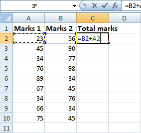
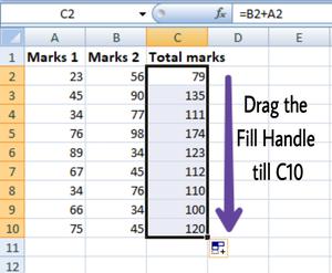
Step 1: We write the formula in any cell and press enter so that it is calculated. In this example, we write the formula(= B2 + A2) in cell C2 and press enter to calculate the formula.
Step 2: Now click on the Fill handle at the corner of cell which contains the formula(C2).

Step 3: Drag the Fill handle up to the cells you want to fill. In our example, we will drag it till cell C10.
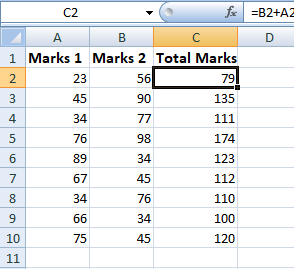
Step 4: Now we can see that the addition operation is performed between the cell A2 and B2, A3 and B3 and so on.
Step 5: You can double-click on any cell to check that the operation is performed in between which cells.
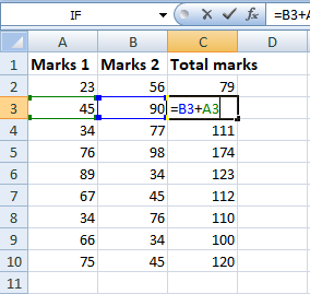
Thus, in the above example, we see that the relative address of cell A2 changes to A3, A4, and so on, similarly the relative address changes for column B, depending on the relative position of the row.
Absolute Reference
Absolute reference is the cell reference in which the row and column are made constant by adding the dollar ($) sign before the column name and row number. The absolute reference does not change as you copy the formula from one cell to other. If either the row or the column is made constant then it is known as a mixed reference. You can also press the F4 key to make any cell reference constant. $A$1, $B$3 are examples of absolute cell reference.
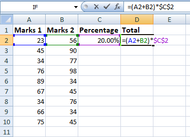
For example, We want to multiply the sum of marks of two subjects, entered in column A and column B, with the percentage entered in cell C2 and display the result in column D. Here, we will use absolute reference so that the address of cell C2 remains constant and does not change with the relative position of column and rows.
Steps to Use Absolute Reference:
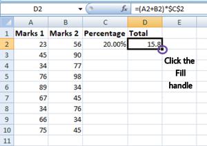
Step 1: We write the formula in any cell and press enter so that it is calculated. In this example, we write the formula(=(A2+B2)*$C$2) in cell D2 and press enter to calculate the formula.
Step 2: Now click on the Fill handle at the corner of cell which contains the formula(D2).
Step 3: Drag the Fill handle up to the cells you want to fill. In our example, we will drag it till cell D10.
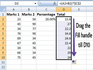
Step 4: Now we can see that the percentage is calculated in column D.
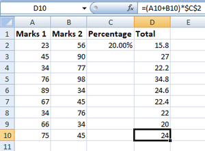
Step 5: You can double-click on any cell to check that the operation is performed in between which cells, and we see that the address of cell C2 does not change.
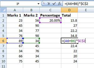
Thus, in the above example we see that the address of cell C2 is not changed whereas the address of column A and B changes with the relative position of the row and column, this happened because we used the absolute address of the cell C2.
Excel Relative References
Relative and Absolute References
Cells in Excel have unique references, which is its location.
References are used in formulas to do calculations, and the fill function can be used to continue formulas sidewards, downwards and upwards.
Excel has two types of references:
- Relative references
- Absolute references
Absolute reference is a choice we make. It is a command which tells Excel to lock a reference.
The dollar sign ($) is used to make references absolute.
Example of relative reference: A1
Example of absolute reference: $A$1
Relative reference
References are relative by default, and are without dollar sign ($).
The relative reference makes the cells reference free. It gives the fill function freedom to continue the order without restrictions.
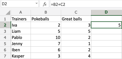
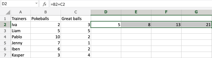
Let’s have a look at a relative reference example, helping the Pokemon trainers to count their Pokeballs (B2:B7) and Great balls (C2:C7).
The result is: D2(5):
Next, fill the range D2:D7:
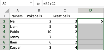
The references being relative allows the fill function to continue the formula for rows downwards.
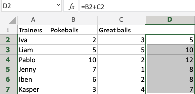
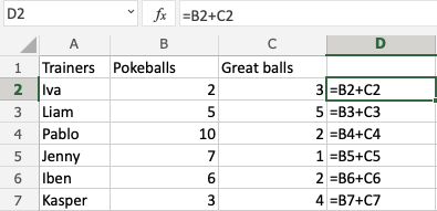
Have a look at the formulas in D2:D7. Notice that it calculates the next row as you fill.
A Non-Working Example
Let’s try an example that will not work.
Fill D2:G2, filling to the right instead of downwards. Resulting in strange numbers:
Have a look at the formulas.
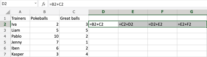
It assumes that we are calculating sidewards and not downwards.
The numbers that we want to calculate need to be in the same direction as we fill.
Test Yourself With Exercises
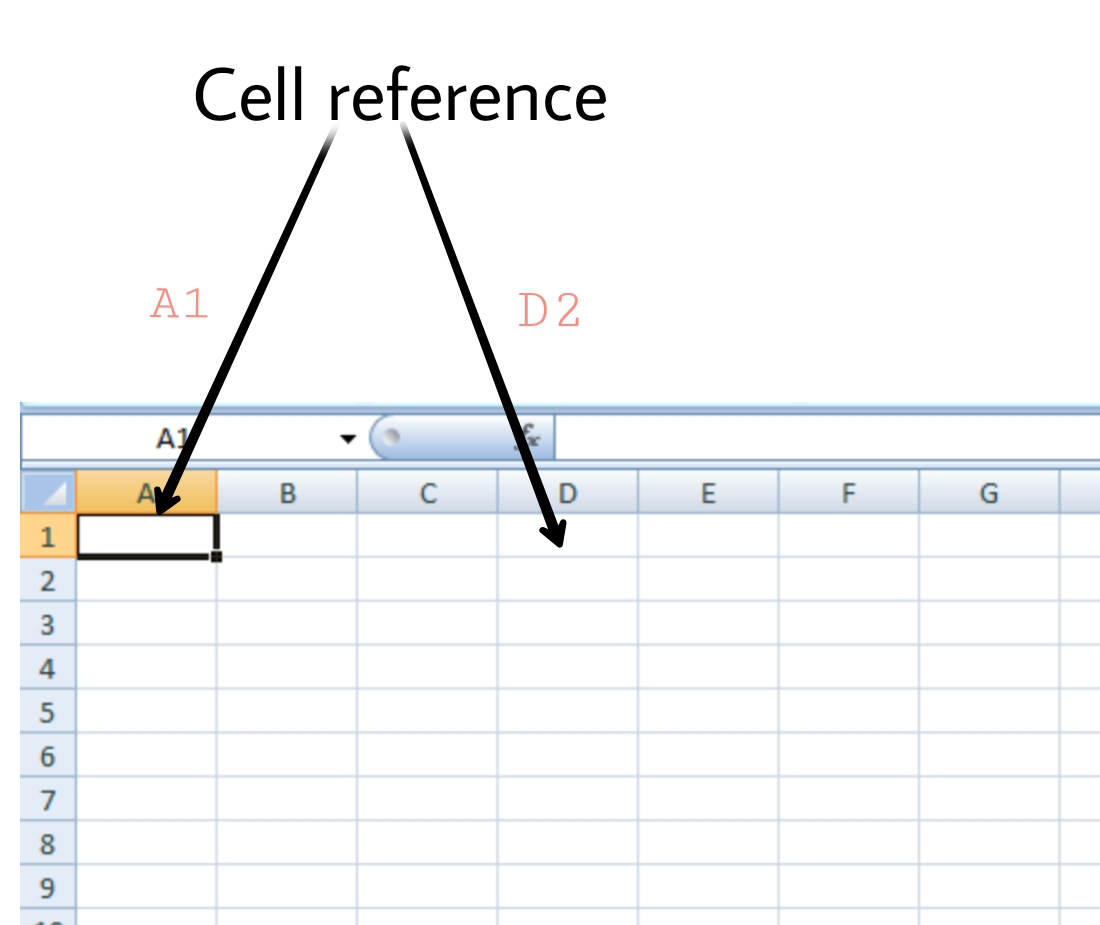
A worksheet in Excel is made up of cells. These cells can be referenced by specifying the row value and the column value.
For example, A1 would refer to the first row (specified as 1) and the first column (specified as A). Similarly, B3 would be the third row and second column.
The power of Excel lies in the fact that you can use these cell references in other cells when creating formulas.
Now there are three kinds of cell references that you can use in Excel:
- Relative Cell References
- Absolute Cell References
- Mixed Cell References
Understanding these different types of cell references will help you work with formulas and save time (especially when copy-pasting formulas).
What are Relative Cell References in Excel?
Let me take a simple example to explain the concept of relative cell references in Excel.
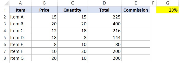
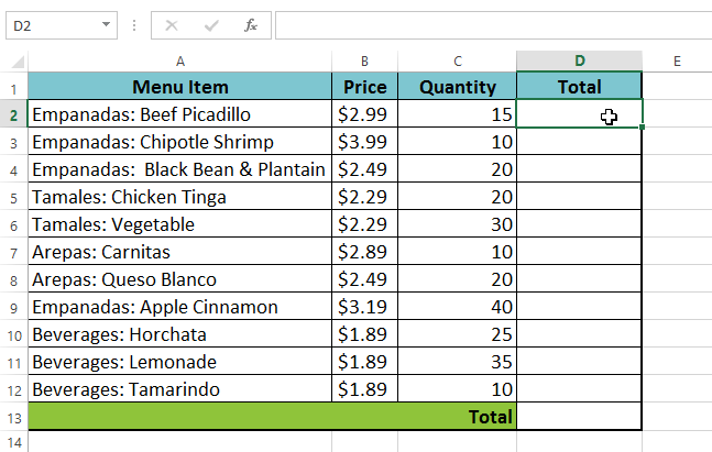
Suppose I have a data set shown below:
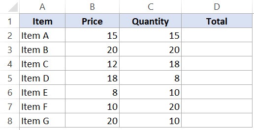
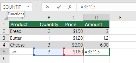
To calculate the total for each item, we need to multiply the price of each item with the quantity of that item.
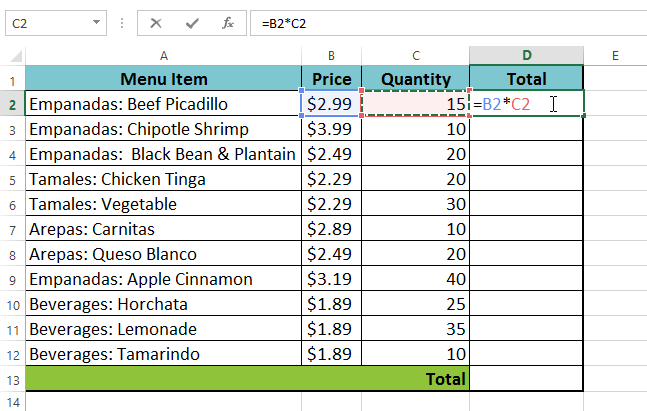
For the first item, the formula in cell D2 would be B2* C2 (as shown below):
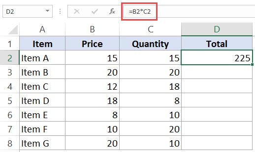
Now, instead of entering the formula for all the cells one by one, you can simply copy cell D2 and paste it into all the other cells (D3:D8). When you do it, you will notice that the cell reference automatically adjusts to refer to the corresponding row. For example, the formula in cell D3 becomes B3*C3 and the formula in D4 becomes B4*C4.
These cell references that adjust itself when the cell is copied are called relative cell references in Excel.
When to Use Relative Cell References in Excel?
Relative cell references are useful when you have to create a formula for a range of cells and the formula needs to refer to a relative cell reference.
In such cases, you can create the formula for one cell and copy-paste it into all cells.
What are Absolute Cell References in Excel?
Unlike relative cell references, absolute cell references don’t change when you copy the formula to other cells.
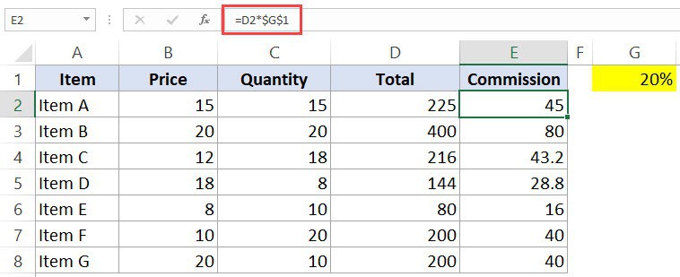
For example, suppose you have the data set as shown below where you have to calculate the commission for each item’s total sales.
The commission is 20% and is listed in cell G1.
To get the commission amount for each item sale, use the following formula in cell E2 and copy for all cells:
=D2*$G$1
Note that there are two dollar signs ($) in the cell reference that has the commission – $G$2.
What does the Dollar ($) sign do?
A dollar symbol, when added in front of the row and column number, makes it absolute (i.e., stops the row and column number from changing when copied to other cells).
For example, in the above case, when I copy the formula from cell E2 to E3, it changes from =D2*$G$1 to =D3*$G$1.
Note that while D2 changes to D3, $G$1 doesn’t change.
Since we have added a dollar symbol in front of ‘G’ and ‘1’ in G1, it wouldn’t let the cell reference change when it’s copied.
Hence this makes the cell reference absolute.
When to Use Absolute Cell References in Excel?
Absolute cell references are useful when you don’t want the cell reference to change as you copy formulas. This could be the case when you have a fixed value that you need to use in the formula (such as tax rate, commission rate, number of months, etc.)
While you can also hard code this value in the formula (i.e., use 20% instead of $G$2), having it in a cell and then using the cell reference allows you to change it at a future date.
For example, if your commission structure changes and you’re now paying out 25% instead of 20%, you can simply change the value in cell G2, and all the formulas would automatically update.
What are Mixed Cell References in Excel?
Mixed cell references are a bit more tricky than the absolute and relative cell references.
There can be two types of mixed cell references:
- The row is locked while the column changes when the formula is copied.
- The column is locked while the row changes when the formula is copied.
Let’s see how it works using an example.
Below is a data set where you need to calculate the three tiers of commission based on the percentage value in cell E2, F2, and G2.
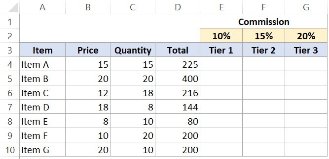
Now you can use the power of mixed reference to calculate all these commissions with just one formula.
Enter the below formula in cell E4 and copy for all cells.
=$B4*$C4*E$2
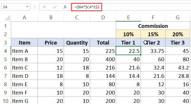
The above formula uses both kinds of mixed cell references (one where the row is locked and one where the column is locked).
Let’s analyze each cell reference and understand how it works:
- $B4 (and $C4) – In this reference, the dollar sign is right before the Column notation but not before the Row number. This means that when you copy the formula to the cells on the right, the reference will remain the same as the column is fixed. For example, if you copy the formula from E4 to F4, this reference would not change. However, when you copy it down, the row number would change as it is not locked.
- E$2 – In this reference, the dollar sign is right before the row number, and the Column notation has no dollar sign. This means that when you copy the formula down the cells, the reference will not change as the row number is locked. However, if you copy the formula to the right, the column alphabet would change as it’s not locked.
How to Change the Reference from Relative to Absolute (or Mixed)?
To change the reference from relative to absolute, you need to add the dollar sign before the column notation and the row number.
For example, A1 is a relative cell reference, and it would become absolute when you make it $A$1.
If you only have a couple of references to change, you may find it easy to change these references manually. So you can go to the formula bar and edit the formula (or select the cell, press F2, and then change it).
However, a faster way to do this is by using the keyboard shortcut – F4.
When you select a cell reference (in the formula bar or in the cell in edit mode) and press F4, it changes the reference.
Suppose you have the reference =A1 in a cell.
Here is what happens when you select the reference and press the F4 key.
- Press F4 key once: The cell reference changes from A1 to $A$1 (becomes ‘absolute’ from ‘relative’).
- Press F4 key two times: The cell reference changes from A1 to A$1 (changes to mixed reference where the row is locked).
- Press F4 key three times: The cell reference changes from A1 to $A1 (changes to mixed reference where the column is locked).
- Press F4 key four times: The cell reference becomes A1 again.
You May Also Like the Following Excel Tutorials:
- How to Copy and Paste Formulas in Excel without Changing Cell References
- How to Lock Cells in Excel.
- Excel Freeze Panes: Use it to Lock Row/Column Headers.
- How to Lock Formulas in Excel.
- How to Reference Another Sheet or Workbook in Excel
- How to Find Circular Reference in Excel
- Using A1 or R1C1 Reference Notation in Excel (& How to Change These)
Содержание
- Определение абсолютных и относительных ссылок
- Пример относительной ссылки
- Ошибка в относительной ссылке
- Создание абсолютной ссылки
- Смешанные ссылки
- Вопросы и ответы

При работе с формулами в программе Microsoft Excel пользователям приходится оперировать ссылками на другие ячейки, расположенные в документе. Но, не каждый пользователь знает, что эти ссылки бывают двух видов: абсолютные и относительные. Давайте выясним, чем они отличаются между собой, и как создать ссылку нужного вида.
Определение абсолютных и относительных ссылок
Что же представляют собой абсолютные и относительные ссылки в Экселе?
Абсолютные ссылки – это ссылки, при копировании которых координаты ячеек не изменяются, находятся в зафиксированном состоянии. В относительных ссылках координаты ячеек изменяются при копировании, относительно других ячеек листа.
Пример относительной ссылки
Покажем, как это работает на примере. Возьмем таблицу, которая содержит количество и цену различных наименований продуктов. Нам нужно посчитать стоимость.
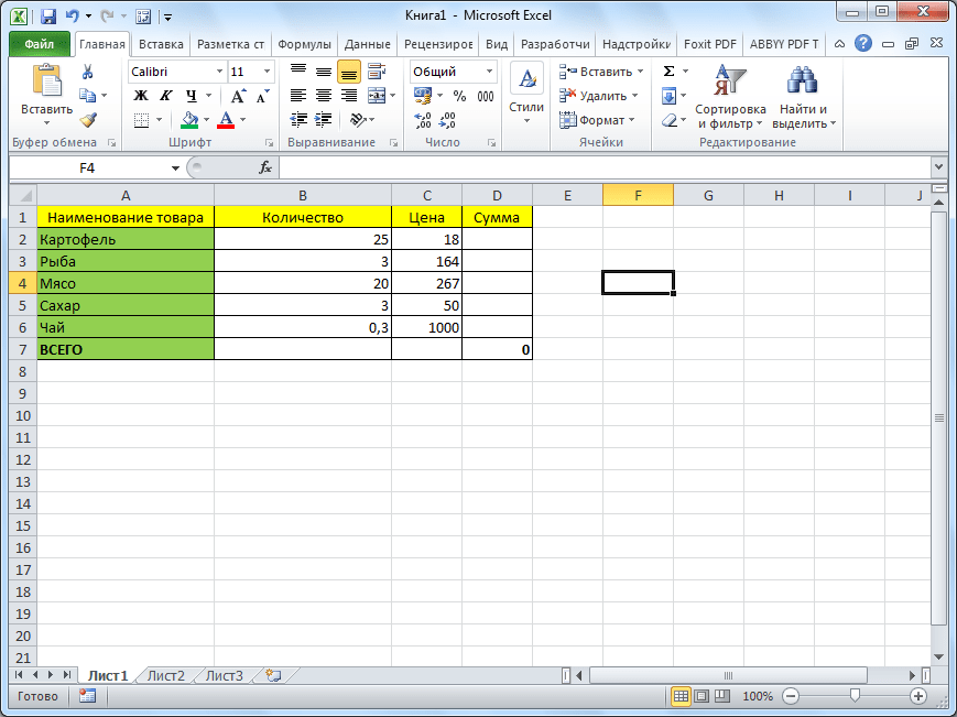
Делается это простым умножением количества (столбец B) на цену (столбец C). Например, для первого наименования товара формула будет выглядеть так «=B2*C2». Вписываем её в соответствующую ячейку таблицы.

Теперь, чтобы вручную не вбивать формулы для ячеек, которые расположены ниже, просто копируем данную формулу на весь столбец. Становимся на нижний правый край ячейки с формулой, кликаем левой кнопкой мыши, и при зажатой кнопке тянем мышку вниз. Таким образом, формула скопируется и в другие ячейки таблицы.

Но, как видим, формула в нижней ячейке уже выглядит не «=B2*C2», а «=B3*C3». Соответственно, изменились и те формулы, которые расположены ниже. Вот таким свойством изменения при копировании и обладают относительные ссылки.

Ошибка в относительной ссылке
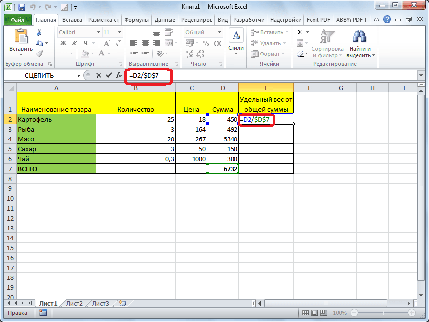
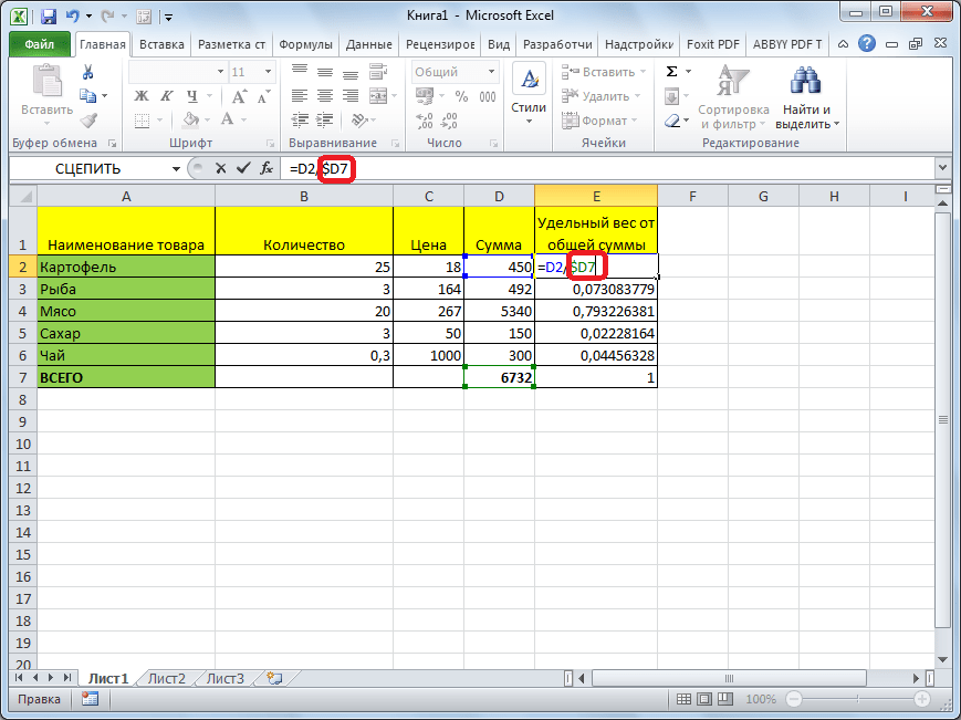
Но, далеко не во всех случаях нам нужны именно относительные ссылки. Например, нам нужно в той же таблице рассчитать удельный вес стоимости каждого наименования товара от общей суммы. Это делается путем деления стоимости на общую сумму. Например, чтобы рассчитать удельный вес картофеля, мы его стоимость (D2) делим на общую сумму (D7). Получаем следующую формулу: «=D2/D7».
В случае, если мы попытаемся скопировать формулу в другие строки тем же способом, что и предыдущий раз, то получим совершенно неудовлетворяющий нас результат. Как видим, уже во второй строке таблицы формула имеет вид «=D3/D8», то есть сдвинулась не только ссылка на ячейку с суммой по строке, но и ссылка на ячейку, отвечающую за общий итог.


D8 – это совершенно пустая ячейка, поэтому формула и выдаёт ошибку. Соответственно, формула в строке ниже будет ссылаться на ячейку D9, и т.д. Нам же нужно, чтобы при копировании постоянно сохранялась ссылка на ячейку D7, где расположен итог общей суммы, а такое свойство имеют как раз абсолютные ссылки.
Создание абсолютной ссылки
Таким образом, для нашего примера делитель должен быть относительной ссылкой, и изменяться в каждой строке таблицы, а делимое должно быть абсолютной ссылкой, которая постоянно ссылается на одну ячейку.
С созданием относительных ссылок у пользователей проблем не будет, так как все ссылки в Microsoft Excel по умолчанию являются относительными. А вот, если нужно сделать абсолютную ссылку, придется применить один приём.
После того, как формула введена, просто ставим в ячейке, или в строке формул, перед координатами столбца и строки ячейки, на которую нужно сделать абсолютную ссылку, знак доллара. Можно также, сразу после ввода адреса нажать функциональную клавишу F7, и знаки доллара перед координатами строки и столбца отобразятся автоматически. Формула в самой верхней ячейке примет такой вид: «=D2/$D$7».
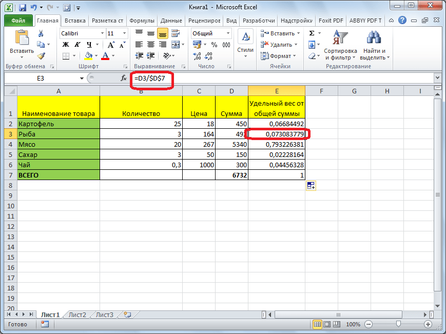
Копируем формулу вниз по столбцу. Как видим, на этот раз все получилось. В ячейках находятся корректные значения. Например, во второй строке таблицы формула выглядит, как «=D3/$D$7», то есть делитель поменялся, а делимое осталось неизменным.
Смешанные ссылки
Кроме типичных абсолютных и относительных ссылок, существуют так называемые смешанные ссылки. В них одна из составляющих изменяется, а вторая фиксированная. Например, у смешанной ссылки $D7 строчка изменяется, а столбец фиксированный. У ссылки D$7, наоборот, изменяется столбец, но строчка имеет абсолютное значение.
Как видим, при работе с формулами в программе Microsoft Excel для выполнения различных задач приходится работать как с относительными, так и с абсолютными ссылками. В некоторых случаях используются также смешанные ссылки. Поэтому, пользователь даже среднего уровня должен четко понимать разницу между ними, и уметь пользоваться этими инструментами.
Lesson 4: Relative and Absolute Cell References
/en/excelformulas/complex-formulas/content/
Introduction
There are two types of cell references: relative and absolute. Relative and absolute references behave differently when copied and filled to other cells. Relative references change when a formula is copied to another cell. Absolute references, on the other hand, remain constant no matter where they are copied.
Optional: Download our example file for this lesson.
Watch the video below to learn more about cell references.
Relative references
By default, all cell references are relative references. When copied across multiple cells, they change based on the relative position of rows and columns. For example, if you copy the formula =A1+B1 from row 1 to row 2, the formula will become =A2+B2. Relative references are especially convenient whenever you need to repeat the same calculation across multiple rows or columns.
To create and copy a formula using relative references:
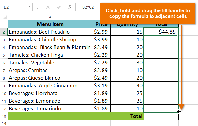
In the following example, we want to create a formula that will multiply each item’s price by the quantity. Rather than create a new formula for each row, we can create a single formula in cell D2 and then copy it to the other rows. We’ll use relative references so the formula correctly calculates the total for each item.
- Select the cell that will contain the formula. In our example, we’ll select cell D2.

- Enter the formula to calculate the desired value. In our example, we’ll type =B2*C2.
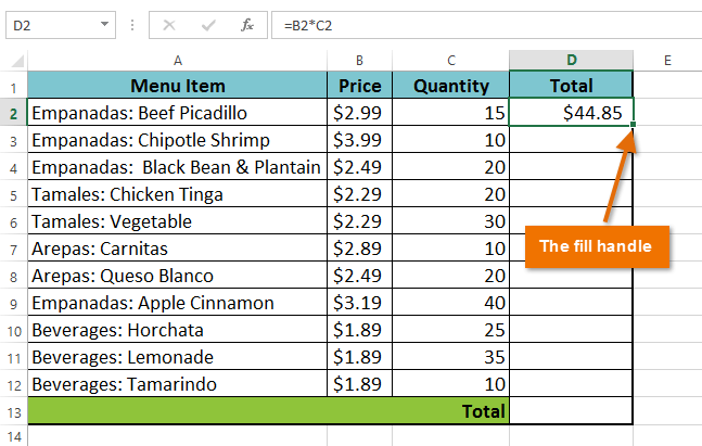
- Press Enter on your keyboard. The formula will be calculated, and the result will be displayed in the cell.
- Locate the fill handle in the lower-right corner of the desired cell. In our example, we’ll locate the fill handle for cell D2.
- Click, hold, and drag the fill handle over the cells you wish to fill. In our example, we’ll select cells D3:D12.
- Release the mouse. The formula will be copied to the selected cells with relative references and the values will be calculated in each cell.
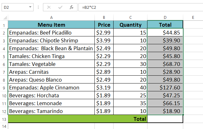
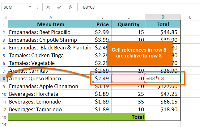
You can double-click the filled cells to check their formulas for accuracy. The relative cell references should be different for each cell, depending on its row.
Absolute references
There may be times when you do not want a cell reference to change when filling cells. Unlike relative references, absolute references do not change when copied or filled. You can use an absolute reference to keep a row and/or column constant.
An absolute reference is designated in a formula by the addition of a dollar sign ($) before the column and row. If it precedes the column or row (but not both), it’s known as a mixed reference.
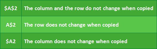
You will use the relative (A2) and absolute ($A$2) formats in most formulas. Mixed references are used less frequently.
When writing a formula in Microsoft Excel, you can press the F4 key on your keyboard to switch between relative, absolute, and mixed cell references, as shown in the video below. This is an easy way to quickly insert an absolute reference.
To create and copy a formula using absolute references:
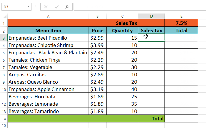
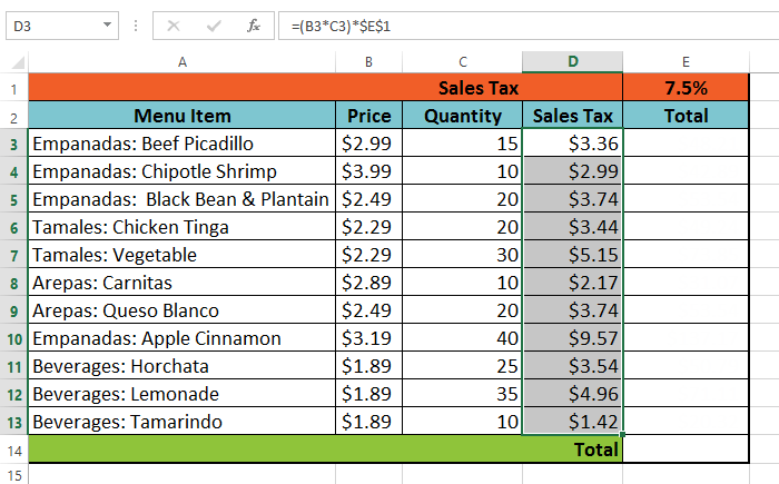
In our example, we’ll use the 7.5% sales tax rate in cell E1 to calculate the sales tax for all items in column D. We’ll need to use the absolute cell reference $E$1 in our formula. Because each formula is using the same tax rate, we want that reference to remain constant when the formula is copied and filled to other cells in column D.
- Select the cell that will contain the formula. In our example, we’ll select cell D3.

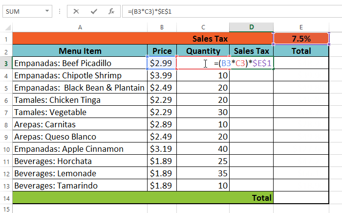
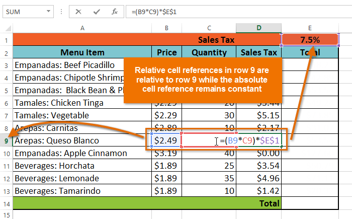
- Enter the formula to calculate the desired value. In our example, we’ll type =(B3*C3)*$E$1.

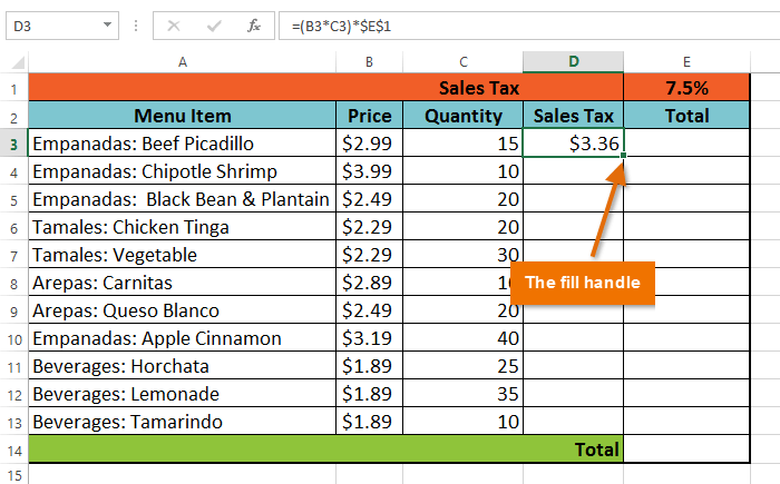
- Press Enter on your keyboard. The formula will calculate, and the result will display in the cell.
- Locate the fill handle in the lower-right corner of the desired cell. In our example, we’ll locate the fill handle for cell D3.
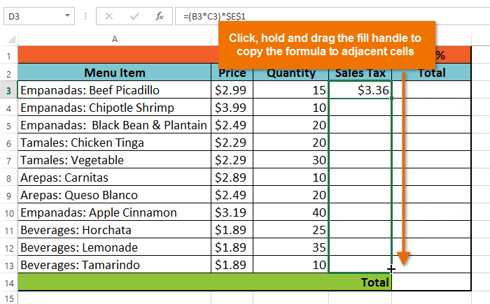
- Click, hold, and drag the fill handle over the cells you wish to fill, cells D4:D13 in our example.
- Release the mouse. The formula will be copied to the selected cells with an absolute reference, and the values will be calculated in each cell.
You can double-click the filled cells to check their formulas for accuracy. The absolute reference should be the same for each cell, while the other references are relative to the cell’s row.
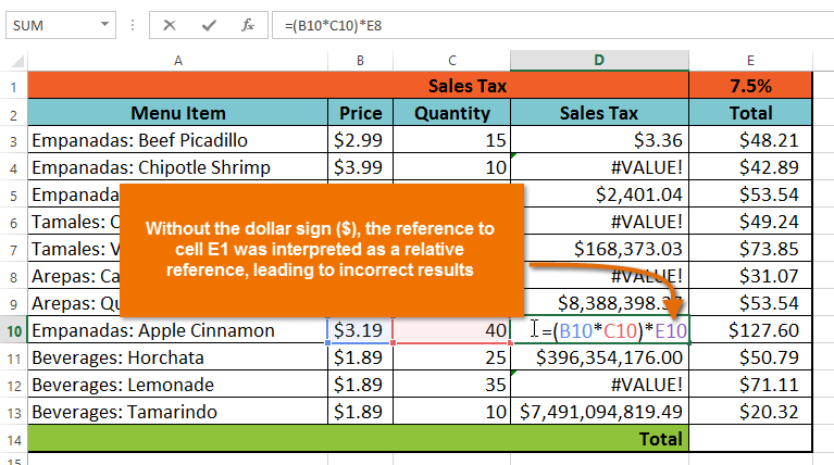
Be sure to include the dollar sign ($) whenever you’re making an absolute reference across multiple cells. The dollar signs were omitted in the example below. This caused the spreadsheet to interpret it as a relative reference, producing an incorrect result when copied to other cells.
Using cell references with multiple worksheets
Most spreadsheet programs allow you to refer to any cell on any worksheet, which can be especially helpful if you want to reference a specific value from one worksheet to another. To do this, you’ll simply need to begin the cell reference with the worksheet name followed by an exclamation point (!). For example, if you wanted to reference cell A1 on Sheet1, its cell reference would be Sheet1!A1.
Note that if a worksheet name contains a space, you will need to include single quotation marks (‘ ‘) around the name. For example, if you wanted to reference cell A1 on a worksheet named July Budget, its cell reference would be ‘July Budget’!A1.
To reference cells across worksheets:
In our example below, we’ll refer to a cell with a calculated value between two worksheets. This will allow us to use the exact same value on two different worksheets without rewriting the formula or copying data between worksheets.
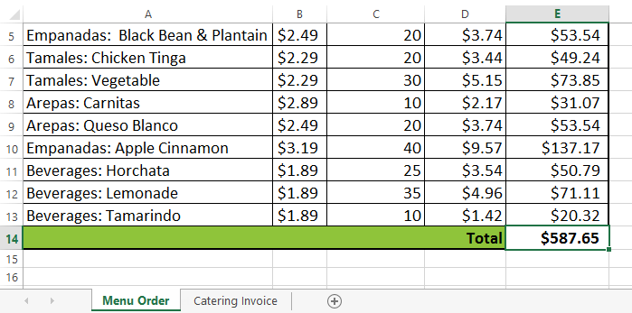
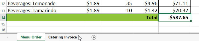
- Locate the cell you wish to reference, and note its worksheet. In our example, we want to reference cell E14 on the Menu Order worksheet.

- Navigate to the desired worksheet. In our example, we’ll select the Catering Invoice worksheet.

- The selected worksheet will appear.
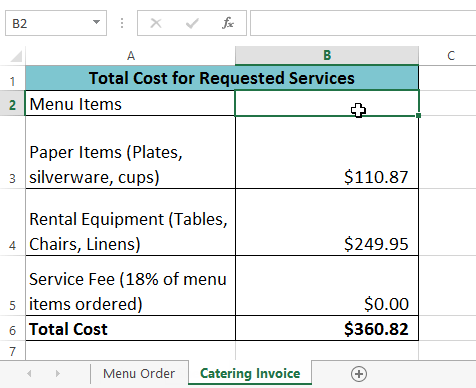
- Locate and select the cell where you want the value to appear. In our example, we’ll select cell B2.

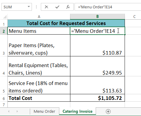
- Type the equals sign (=), the sheet name followed by an exclamation point (!), and the cell address. In our example, we’ll type =’Menu Order’!E14.

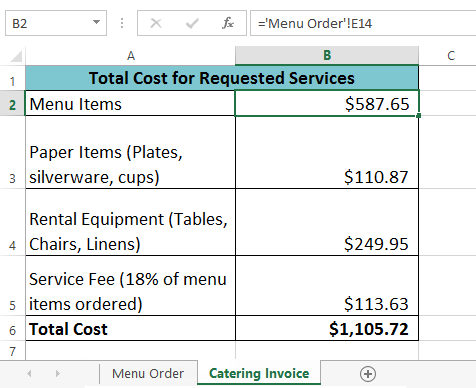
- Press Enter on your keyboard. The value of the referenced cell will appear. If the value of cell E14 changes on the Menu Order worksheet, it will be updated automatically on the Catering Invoice worksheet.
If you rename your worksheet at a later point, the cell reference will be updated automatically to reflect the new worksheet name.
Challenge!
- Open an existing Excel workbook. If you want, you can use the example file for this lesson.
- Create a formula that uses a relative reference. If you are using the example, use the fill handle to fill in the formula in cells E4 through E14. Double-click a cell to see the copied formula and the relative cell references.
- Create a formula that uses an absolute reference. If you are using the example, correct the formula in cell D4 to refer only to the tax rate in cell E2 as an absolute reference, then use the fill handle to fill the formula from cells D4 to D14.
- Try referencing a cell across worksheets. If you are using the example, create a cell reference in cell B3 on the Catering Invoice worksheet for cell E15 on the Menu Order worksheet.
/en/excelformulas/functions/content/
While working or learning Excel, you’ve must hear of Relative and Absolute referencing of cells and ranges. Absolute referencing is also called locking of cells. Understanding of Relative and Absolute Reference in Excel is very important to work effectively on Excel. So let’s get started.
Absolute Referencing or Locking Cell in Formula
When you don’t want to change the referenced cell while you copy a formula cell somewhere else, you use Absolute Referencing using $ sign. Let’s see an example.
Create A Table Generator
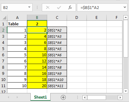
In this example, you need to create a table generator. You will write a number in Cell B1. The Range B2: B11 should display the table of that number.
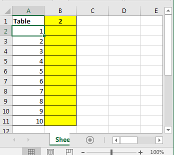
You just need to multiply B1 to A1 and then just copy the formula below. It won’t work my friend but let’s just try this…
In cell B2, write this formula and copy it in below cell.
=B1*A2
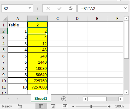
What happened? ???? This is not the table of 2 you learned in primary school. Ok lets see whats going on here.
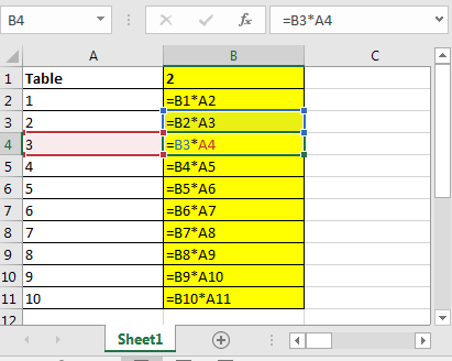
When copy or drag down the formula cell, the reference to B1 also changes. See below image.
This is called Relative Referencing. So how do we lock cell B2 or say give an Absolute Reference of a cell?
- Just put a $ sign before column character and row number to lock the cell in excel. Eg. ($A$1).
- Or select the range in formula and hit F4 button.
The formula in cell B2 will look like this.
=$B$1*A2
Copy it to the below cells or anywhere else. The reference to B1 will not change.
Relative Referencing or Locking Cell in Formula
In the above example, the reference to cell A2 is relative. The relative cell changes relatively when the formula is copied to another cell. As happens to A2 in the above example. Where the cell B2 is copied to B3 the reference of A2 changes to A3.
You can make row absolute and column relative or vice versa by just putting $ sign before a column or row number.
For example eg; $A1 means the only column a is locked but the row is not. If you copy this cell to left the column A will not change but when to copy the formula down the row number will change.
Related Articles:
How to use Dynamic Worksheet Reference in Excel
How to use Relative and Absolute Reference in Excel in Excel
How to use Shortcut To Toggle Between Absolute and Relative References in Excel
How to Count Unique Values In Excel
All About Excel Named Ranges in Excel
Popular Articles:
50 Excel Shortcuts to Increase Your Productivity
How to use the VLOOKUP Function in Excel
How to use the COUNTIF function in Excel
How to use the SUMIF Function in Excel
Содержание
- Switch between relative, absolute, and mixed references
- Cell References in Excel – Relative, Absolute, Mixed
- What is a Cell Reference?
- For example:
- Types of Cell Reference in Excel
- 1. Relative Cell Reference
- How to Use Relative Cell References in Excel
- #Example 1:
- #Example 2:
- When to Use Relative Cell References in Excel
- 2. Absolute Cell Reference
- How to Use Absolute Cell References in Excel
- #Example:
- What Does the Dollar ($) Sign Do?
- When to Use Absolute Cell References in Excel
- 3. Mixed Cell Reference
- #Example:
- Some Other Ways of Using Cell References With Examples
- Relative and Absolute Cell References for Calculating Dates
- Whole Column Reference
- Whole Row Reference
- Refer to an Entire Column, Excluding the First Few Rows
- Using a Mixed Entire Column Reference in Excel
- How to switch between Absolute, Relative, and Mixed References
- Important Points to Remember
- FAQs on Excel Cell References
- 1. What are the 3 types of cell references in Excel?
- Relative, Absolute, and Mixed Cell References in Excel and Sheets
- In This Article
- The Different Types of Cell References
- How Cell References Use Automatic Updating
- You Can Reference Cells From Different Worksheets
- Cell Range: A Quick Primer
- Copying Formulas and Different Cell References
- Toggling Between Types of Cell References
Switch between relative, absolute, and mixed references
By default, a cell reference is a relative reference, which means that the reference is relative to the location of the cell. If, for example, you refer to cell A2 from cell C2, you are actually referring to a cell that is two columns to the left (C minus A)—in the same row (2). When you copy a formula that contains a relative cell reference, that reference in the formula will change.
As an example, if you copy the formula =B4*C4 from cell D4 to D5, the formula in D5 adjusts to the right by one column and becomes =B5*C5. If you want to maintain the original cell reference in this example when you copy it, you make the cell reference absolute by preceding the columns (B and C) and row (2) with a dollar sign ( $). Then, when you copy the formula =$B$4*$C$4 from D4 to D5, the formula stays exactly the same.
Less often, you may want to mixed absolute and relative cell references by preceding either the column or the row value with a dollar sign—which fixes either the column or the row (for example, $B4 or C$4).
To change the type of cell reference:
Select the cell that contains the formula.
In the formula bar  , select the reference that you want to change.
Press F4 to switch between the reference types.
The table below summarizes how a reference type updates if a formula containing the reference is copied two cells down and two cells to the right.
Источник
Cell References in Excel – Relative, Absolute, Mixed
Microsoft Excel, sometimes known as MS Excel, is a potent spreadsheet programme. In Excel, each worksheet consists of a number of cells that are made up of rows and columns. Each cell has a unique reference, which enables users to quickly access and address the required cell (or cells) within the functions. In Excel, cell references are crucial, particularly when working with huge data sets in functions and formulas.
This article covers a quick overview of Excel Cell References. The various sorts of cell references that Excel offers and the detailed instructions for using each one are also covered in the article.
What is a Cell Reference?
An Excel cell reference, also known as a cell address, is a mechanism that defines a cell on a worksheet by combining a column letter and a row number. We can refer to any cell (in Excel formulas) in the worksheet by using the cell references.
For example:
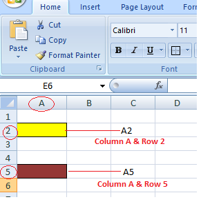
Here we refer to the cell in column A & row 2 by A2 & cell in column A & row 5 by A5. You can make use of such notations in any of the formulas or copy the value of one cell to another cell (by using = A2 or = A5).
Types of Cell Reference in Excel
Understanding various cell references primarily makes it easier for us to use Excel formulas and avoid unexpected formula errors. When copying and pasting Excel formulas, this is quite useful. Based on various use situations, Excel offers three main types of cell references, including:
- Relative Cell Reference
- Absolute Cell Reference
- Mixed Cell Reference
1. Relative Cell Reference
In Excel, a relative cell reference is used by default. Excel uses a relative reference whenever we insert a cell reference or a range within a formula. The relative references, which commonly reflect the combination of column name and row number, are used normally with the associated cell references. There is no dollar ($) sign in the relative reference for the cell.
How to Use Relative Cell References in Excel
Let’s see how to use the Relative Cell references through examples,
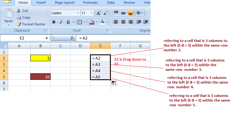
#Example 1:
If you refer to cell B1 from cell E1, actually you would be referring to a cell that is 3 columns to the left (E-B = 3) within the same row number 1.
When it is copied to other locations present in a worksheet, the relative reference for that location will be changed automatically. (because relative cell reference describes offset to another cell rather than a fixed address as In our example, offset is : 3 columns left in the same row).
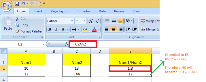
#Example 2:
If you copy the formula = C2 / A2 from the cell “E2” to “E3”, the formula in E3 will automatically become =C3/A3.
When to Use Relative Cell References in Excel
When you need to develop a formula for a set of cells and the formula needs to make a reference to a relative cell reference, relative cell references come in handy.
When this occurs, you can create the formula in one cell and copy it before pasting it into every other cell.
2. Absolute Cell Reference
When copying or using AutoFill, there are times when the cell reference must stay the same. A column and/or row reference is kept constant using dollar signs. So, to get an absolute reference from a relative, we can use the dollar sign ($) characters.
To refer to an actual fixed location on a worksheet whenever copying is done, we use absolute reference. The reference here is locked such that rows and columns do not shift when copied.
How to Use Absolute Cell References in Excel
Below is an example depicting how to use Absolute Cell References in Excel.
#Example:
When we fix both row & column – Say if we want to lock row 2 & column A, we will use $A$2 as:
G2 = C2/$A$2, when copied to G3, G3 becomes = C3/$A$2
Note: C3 is 4 columns left to G3 in the same row.
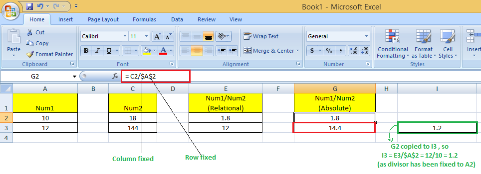
Here, original cell reference A2 is maintained whenever we copy G2 to any of the cells. So I3 = E3/$A$2 because E3 comes from the relative reference (4 columns left to the current one) & /$A$2 comes from the absolute reference.
Therefore, I3 = E3//$A$2 = 12/10 = 1.2
What Does the Dollar ($) Sign Do?
When the row and column numbers are preceded by the dollar symbol ($), it becomes absolute (i.e., stops the row and column number from changing when copied to other cells). Dollar ($) before the row fixes the row & before the column fixes the column.
When to Use Absolute Cell References in Excel
When you don’t want the cell reference to alter when you replicate formulas, absolute cell references come in handy. This can be the situation if you have to use a fixed value in the formula.
3. Mixed Cell Reference
An absolute column and relative row, or an absolute row and relative column, is a mixed cell reference. You get an absolute column or absolute row when you individually put the $ before the column letter or before the row number. Example: $B8 is relative to row 8 but absolute for column B, and B$8 is absolute for row 1 but relative for column A.
Here, the Dollar ($) before the row number fixes/locks the row & before the column name fixes/locks the column.
#Example:
When we fix the only row: If we have G2 = C2/A$2 then :
We used $ before the row number, so we are locking the only row here. When G2 is copied to G3, G3 = C3/A$2 (not C3/A3) because the row has been fixed already.
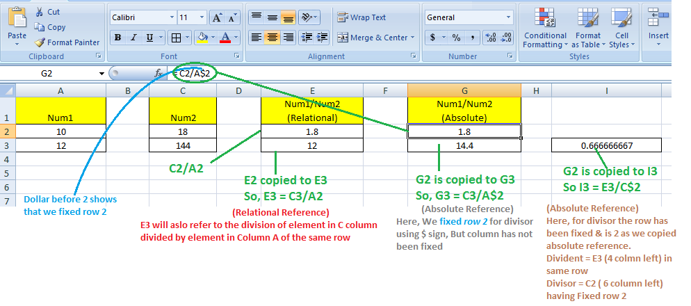
Here, whenever we copy G2 to any other cell, always the divisor will refer to a fixed row 2 (column vary according to the concept of relative reference)
So, when G2 is copied to I3, I3 = E3/C$2 because E3 comes from the relative reference (4 columns left to the current one) & C$2 comes from the absolute reference for row & relative reference for Column (6 Columns left to the current one)
Some Other Ways of Using Cell References With Examples
Now that we are familiar with the basics of using Cell References in Excel, let’s see some other ways of using cell references.
Relative and Absolute Cell References for Calculating Dates
We can use relative and absolute cell references to calculate dates.
Example: To Calculate the Date of Delivery online from the given date of the order placed & no of days it will take to deliver :
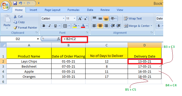
Here, We calculate the Date of Delivery by = Order Date + No of days to deliver. We used Relative cell reference so that individual product delivery dates can be calculated.
Absolute cell references for calculating dates :
Example: To Calculate the Date of Birth When the age is known is a number of days using Current date can be done by making use of absolute reference.
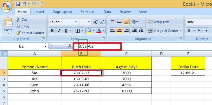
Here, We calculate DOB by = Current Date – Age in days. The Current date is contained in the cell E2 & in subtraction, we fixed that date to subtract from the days.
Whole Column Reference
You will want to refer to all the cells inside a particular column when operating with an Excel worksheet with any number of rows. Simply type a column letter twice with a colon in between to refer to the entire column B, for example, B:B.
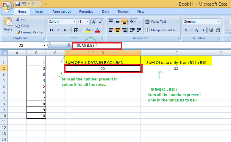
Example: You may want to find the sum of a column of data in certain cases. While you can do this with a regular cell range, such as =SUM(B1:B10), you will need to change the cell range if your spreadsheet grows in size.
Excel, on the other hand, has a cell range that does not require the row number and takes all the cells in the column in action. If you wanted to find the sum of all the values in column B, for example, you would type =SUM (B:B). You can add as much data as you want to your spreadsheet without having to change your cell ranges if you use this type of cell range.
Whole Row Reference
You will want to refer to all the cells inside a particular row when operating with an Excel worksheet with any number of columns. Simply type a row number twice with a colon in between to refer to the entire row, for example, 2:2.
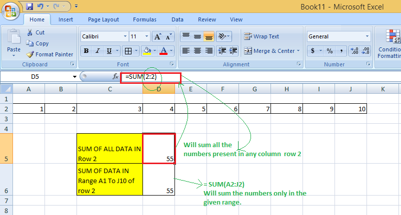
Example: You may want to find the sum of a row of data in certain cases. While you can do this with a regular cell range, such as =SUM(A2 : J2), you will need to change the cell range if your spreadsheet grows in size.
Excel, on the other hand, has a cell range that does not require the column letter and takes all the cells in the row in action. If you wanted to find the sum of all the values in row 2, for example, you would type =SUM (2:2). You can add as much data as you want to your spreadsheet without having to change your cell ranges if you use this type of cell range.
Refer to an Entire Column, Excluding the First Few Rows
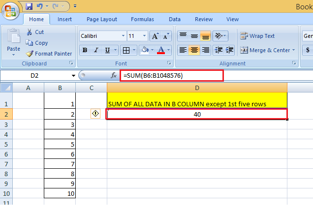
To refer to the entire column excluding the first few rows, you need to specify the range as we give in a normal fashion. We know that the Excel worksheets can have only 1,048,576 rows. (To check this, go to an empty cell & press: Ctrl + Down arrow Key)
So, we can do the sum of the entire column B except for the first 5 rows by = SUM(B6:B1048576).
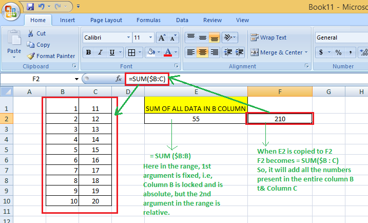
Using a Mixed Entire Column Reference in Excel
You can also create a mixed entire-column reference, say for example $B:B. But, practically, it is difficult to find a situation where it would be used.
Example :
How to switch between Absolute, Relative, and Mixed References
The $ sign can be manually typed in an Excel formula to adjust a relative cell relation to absolute or mixed. You can also speed things up by pressing the F4 key. You must be in formula edit mode to use the F4 shortcut. The steps are :
Firstly, choose the cell that contains the formula. Then, by pressing the F2 key or double-clicking the cell, you can enter Edit mode. Select the cell reference in which you want to make changes. Then, switch between four-cell reference forms by pressing F4.
Example: When you select a cell having only relative reference (i.e., no $ sign), say = B2:
- The first time when you press F4, it becomes =$B$2
- The second time when you press F4, it becomes =B$2
- The third time when you press F4, it becomes=$B2
- The fourth time when you press F4, it becomes back to the relative reference=B2
B2 –Press F4–> =$B$2 –Press F4–> =B$2 –Press F4–> = =$B2 –Press F4–> =B2
So, using F4, you do not require to manually type the $ symbol.
Important Points to Remember
- One of the crucial components for Excel functions or formulas is the cell reference.
- Excel formulas that employ relative cell references automatically change the references to match the correct row and column.
- When copying formulas into non-relative cells, absolute cell references are advised. Excel keeps the absolute cell references constant.
- According to the specifications, a mixed reference only locks one of the references, either the row or the column. Not both are locked.
FAQs on Excel Cell References
1. What are the 3 types of cell references in Excel?
Ans: In Excel, we can use one of three types of cell references:
- Relative Cell References
- Absolute Cell References
- Mixed Cell References
Источник
Relative, Absolute, and Mixed Cell References in Excel and Sheets
In This Article
Jump to a Section
A cell reference in spreadsheet programs such as Excel and Google Sheets identifies the location of a cell in the worksheet. These references use Autofill to adjust and change information as needed in your spreadsheet.
The information in this article applies to Excel versions 2019, 2016, 2013, Excel for Mac, Excel Online, and Google Sheets.
The Different Types of Cell References
The three types of references that can be used in Excel and Google Sheets are easily identified by the presence or absence of dollar signs ($) within the cell reference. A dollar sign tells the program to use that value every time it runs a formula.
- Relative cell references contain no dollar signs (i.e., A1).
- Mixed cell references have dollar signs attached to either the letter or the number in a reference but not both (i.e., $A1 or A$1).
- Absolute cell references have dollar signs attached to each letter or number in a reference (i.e., $A$1).
You’ll typically use an absolute or mixed cell reference if you set up a formula. For example, if you have a number in Cell A1, more numbers in Column B, and Column C contains the sums of A1 and each of the values in B, you’ll use «$A$1» in the SUM formula so that when you autofill, the program knows to always use the number in A1 instead of the empty cells below it.
A cell is one of the boxlike structures that fill a worksheet, and you can locate one by its references, such as A1, F26, or W345. A cell reference consists of the column letter and row number that intersect at the cell’s location. When listing a cell reference, the column letter always appears first. Cell references appear in formulas, functions, charts, and other Excel commands.
How Cell References Use Automatic Updating
One advantage of using cell references in spreadsheet formulas is that, normally, if the data located in the referenced cells changes, the formula or chart automatically updates to reflect the change.
If a workbook has been set not to update automatically when you make changes to a worksheet, you can carry out a manual update by pressing the F9 key on the keyboard.
You Can Reference Cells From Different Worksheets
Cell references are not restricted to the same worksheet where the data is located. Other worksheets in the same file can reference each other by including a notation that tells the program which sheet to pull the cell from.
You don’t need a sheet notation if you’re referring to a cell in the same worksheet.
Similarly, when you reference data in a different workbook, the name of the workbook and the worksheet are included in the reference along with the cell location.
To reference a cell on a different sheet, preface the cell reference with «Sheet[number]» with an exclamation point after it, and then the name of the cell. So if you want to pull info from Cell A1 in Sheet 3, you’ll type, «Sheet3!A1.»
A notation referring to another workbook in Excel also includes the name of the book in brackets. To use the information contained in Cell B2 in Sheet 2 of Workbook 2, you’ll type, «[Book2]Sheet2!B2.»
Cell Range: A Quick Primer
While references often refer to individual cells, such as A1, they can also refer to a group or range of cells. You identify ranges of cells by the starting and ending cells. In the case of ranges that occupy multiple rows and columns, you’ll use the cell references of the cells in the upper left and lower right corners of the range.
Separate the limits of a cell range with a colon ( : ), which tells Excel or Google Sheets to include all the cells between these start and end points. So to grab everything between Cell A1 and D10, you’d type, «A1:D10.»
To capture an entire row or column, you still use the cell range notation, but you only use the column numbers or row letters. To include everything in Column A, the range will be «A:A.» To use Row 8, you’ll type, «8:8.» For everything in Columns B through D, you’ll type, «B:D.»
Copying Formulas and Different Cell References
Another advantage of using cell references in formulas is that they make it easier to copy formulas from one location to another in a worksheet or workbook.
Relative cell references change when copied to reflect the new location of the formula. The name relative comes from the fact that they change relative to their location when copied. This is usually a good thing, and it is why relative cell references are the default type of reference used in formulas.
At times, cell references need to stay static when formulas are copied. Copying formulas is the other major use of an absolute reference such as =$A$2+$A$4. The values in those references don’t change when you copy them.
At other times, you may want part of a cell reference to change, such as the column letter, while having the row number stay static or vice versa when you copy the formula. In this case, you’ll use a mixed cell reference such as =$A2+A$4. Whichever part of the reference has a dollar sign attached to it stays static, while the other part changes when copied.
So for $A2, when it is copied, the column letter is always A, but the row numbers change to $A3, $A4, $A5, and so on.
The decision to use the different cell references when creating the formula is based on the location of the data that the copied formulas will use.
Toggling Between Types of Cell References
The easiest way to change cell references from relative to absolute or mixed is to press the F4 key on the keyboard. To change existing cell references, Excel must be in edit mode, which you enter by double-clicking on a cell with the mouse pointer or by pressing the F2 key on the keyboard.
To convert relative cell references to absolute or mixed cell references:
- Press F4 once to create a cell reference fully absolute, such as $A$6.
- Press F4 a second time to create a mixed reference where the row number is absolute, such as A$6.
- Press F4 a third time to create a mixed reference where the column letter is absolute, such as $A6.
- Press F4 a fourth time to make the cell reference relative again, such as A6.
Get the Latest Tech News Delivered Every Day
Источник
Cell References in Excel: Relative, Absolute, and Mixed (2023)
Cell references often confuse Excel users no matter how simple they may sound.
Be it Cell A1 or Cell XFD1048576. How are these cell references made?🤔
The guide below will teach you this and much more. So jump right in.
And as you go, download our free sample workbook here to practice along the guide.
What are cell references in Excel
Cell references are like the name of cells. A cell reference is alphanumeric; it consists of an alphabet and a number. 🔠
Where do this alphabet and number come from? Here is what a worksheet in Excel looks like (A two-dimensional window with rows and columns).

Columns in Excel are denoted by alphabet. Whereas rows in Excel are denoted by numbers.
A cell is formed at the intersection of a row and a column. It is then named as a combination of that row and column.
For example, in the image below the highlighted cell forms at the intersection of Column B and Row 2.

The highlighted cell is referred to as Cell B2 (Column B and row 2).
Similarly, drag your worksheet to the end to see if even the last cell (Cell XFD1048576) is referred to the same way.

It is formed at the intersection of Column XFD and Row 1048576.
Pro Tip!
Did you know? There are a total of 16,384 columns in Excel. And the total number of rows in Excel is 1,048,576. 💯
How to use cell references (relative references)
Cell references make your Excel jobs unbelievably easy. You can use them everywhere and the best thing – as you move the formulas, the cell reference automatically adjusts.
See here.

The image shows the total marks for each subject in Row 2. The percentage marks acquired by a student in each of these subjects is in Row 3.
Let’s quickly find the marks scored in each subject.
Write the formula in Cell B4 as follows:
= B2 * B3

We are multiplying Cell B2 (Total marks) by Cell B3 (Percentage). Excel calculates the obtained marks in English.

Let’s calculate the same for the remaining subjects. But don’t waste time writing the respective formula for each subject.
Drag and drop the formula in Cell B4 to the remaining cells.

Excel calculates the obtained marks for all the remaining subjects.
But what has Excel done?
When formulas are moved across cells, Excel changes the relative cell references based on the relative rows/columns.
For example, the above formula when copied from Column B to C becomes:
= C2 * C3

Move it from Column C to Column D to see it changes as follows.
= D2 * D3

That way, you do not have to write formulas unique to each cell.
You can put together a single formula for one cell and copy/paste it to the others. Excel will automatically update the relative cell references. 💪
How to use absolute cell references
What if the above data changes as shown below?

The data remains the same. However, marks for each of the subjects are not mentioned now. Instead, we have the total marks in Cell F2 only.
To calculate the marks obtained in English, write the formula below.
= B2 * F2

B2 consists of the percentage marks obtained in English. At the same time, Cell F2 consists of the total marks for all the subjects.
Excel calculates the marks obtained in English as below.

Can we move the same formula (drag and drop it) for the remaining subjects?

The results are bizarre. What has Excel done?

The cell references were relative. As we moved it from one column to another, Excel changed the column reference from F2 to G2. G2 is an empty cell, so, Excel returns zero.
In such a case, we don’t want Excel to change the cell reference (F2) every time the formula is moved. We want to keep it constant.
However, we want the cell reference for percentages to change every time the formula is moved.
Write the formula as follows.
= B2 * $F$2

We have changed the relative reference of Cell F2 into an absolute reference of $F$2.
Unlike relative cell references, an absolute cell reference has a dollar symbol before the column and the row reference. Like $A$1.
However, the cell reference B2 is still the same. This is because we only want to fix the cell reference $F$2 but not B2.
Drag and move it across all the columns

Excel calculates the obtained marks for all the subjects.
This time Excel updated the formula for each next column by changing the cell reference of B2 but not F2.
For example, when moved to Column C, Excel changes the formula as below.

So, the formula changes from:
=INDEX(D:D,MATCH(G2,A:A,0))
To:
=INDEX(D:D,MATCH(1,A:A,0))
The “theory” behind this is not as simple as changing the lookup value.
Since you’re changing the formula from a normal one to an array formula, the structure of the formula changes a bit as well. By changing the lookup value to 1, you’re not actually telling the MATCH function to search for the number 1 in the lookup array (last name column).
Pro Tip!
To change any reference into an absolute cell reference, click on that cell reference in the formula bar and press the F4 key.
Mixed cell referencing in Excel
Who said a cell reference has to be a relative or an absolute one only? There can be mixed cell references too.
Pro Tip!
A mixed cell reference is where any one component of the cell reference (column reference or the row reference) is absolute, and the other is relative.
For example, $C3 (Absolute column reference and relative row reference). Or C$3 (Relative column reference and absolute row reference).
The absolute reference comes after a dollar sign. 💲
For example, the image below the number of units sold for January and February.

To calculate the sales for both months, let’s multiply these by the price.
- Write the formula as:
= B2 * D2

- Drag and drop the same formula to all the products to get the sales for January.

What about February?
- Copy-paste the same formula into the column for February sales.

This is what happens when you do so. As we move the formula one column ahead, Excel changes the column references from B2 and D2 to C2 and E2.

We want Excel to multiply the units sold of each product for each month with the price. This means we want to keep the column of prices (Column D) constant.
- To do so, convert it into a mixed reference as follows.
= C2 * $D2

We only added a dollar sign ($) before the column reference (D). There is no dollar sign ($) before the row reference (2).
This way each time this formula is moved, the column will remain the same (Column D), but the row number would accordingly change.
- Drag and drop the formula now to see the results.

Excel now keeps Column D constant. All other references change with the relative position of the row/column.
Cell references to other worksheets
Cell references are not limited to a single sheet only. You can also create a reference to a cell from another worksheet. 🙌
See here. We have the value for Apples in Sheet 2.

We need this sales value in Sheet 1.
- To create a direct reference to Sheet 2, activate a cell in Sheet 1 and write an equal sign (=).

- Now go to sheet 2 and click on the targeted value (sales value of Apples).

- Press Enter.
- In sheet 1, a reference is created to Cell A2 of Sheet 2.

That is how you can create references to other cells across different worksheets of a workbook.
That’s it – Now what?
Cell references are one of the building blocks of Excel. Unless you understand how cell references work, you can barely use Microsoft Excel.
👉 The above guide teaches you how cell references are formed. We learned about all three types of cell references (mixed, relative, and absolute references). And also how they can be used within a worksheet and across worksheets.
To make your Excel jobs even simpler, you must master the SUMIF, IF, and VLOOKUP functions of Excel.
Click here to sign up for my 30-minute free email course that teaches you these and other functions of Excel.
Other resources
If you enjoyed learning about cell references, we bet you’d love to know more.
Just like cell references, there’s so much more to the basics of Excel that will change the way you work. Hop on here to learn how to select multiple cells and merge/unmerge cells in Excel.
Kasper Langmann2023-01-19T12:13:01+00:00
Page load link