Relative address and absolute address excel - Word и Excel - помощь в работе с программами

Excel for Microsoft 365 Excel for the web Excel 2021 Excel 2019 Excel 2016 Excel 2013 Excel Web App Excel 2010 Excel 2007 More…Less

By default, a cell reference is a relative reference, which means that the reference is relative to the location of the cell. If, for example, you refer to cell A2 from cell C2, you are actually referring to a cell that is two columns to the left (C minus A)—in the same row (2). When you copy a formula that contains a relative cell reference, that reference in the formula will change.

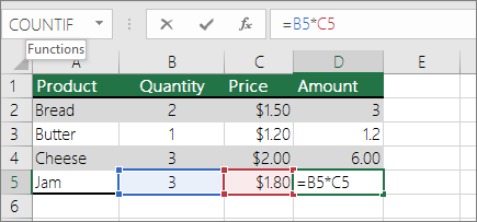
As an example, if you copy the formula =B4*C4 from cell D4 to D5, the formula in D5 adjusts to the right by one column and becomes =B5*C5. If you want to maintain the original cell reference in this example when you copy it, you make the cell reference absolute by preceding the columns (B and C) and row (2) with a dollar sign ($). Then, when you copy the formula =$B$4*$C$4 from D4 to D5, the formula stays exactly the same.

Less often, you may want to mixed absolute and relative cell references by preceding either the column or the row value with a dollar sign—which fixes either the column or the row (for example, $B4 or C$4).

To change the type of cell reference:

Select the cell that contains the formula.
In the formula bar , select the reference that you want to change.
Press F4 to switch between the reference types.

The table below summarizes how a reference type updates if a formula containing the reference is copied two cells down and two cells to the right.

For a formula being copied:	If the reference is:	It changes to:
	$A$1 (absolute column and absolute row)	$A$1 (the reference is absolute)
	A$1 (relative column and absolute row)	C$1 (the reference is mixed)
	$A1 (absolute column and relative row)	$A3 (the reference is mixed)
	A1 (relative column and relative row)	C3 (the reference is relative)

Need more help?

Want more options?

Explore subscription benefits, browse training courses, learn how to secure your device, and more.

Communities help you ask and answer questions, give feedback, and hear from experts with rich knowledge.

Источник

Cell reference is the address or name of a cell or a range of cells. It is the combination of column name and row number. It helps the software to identify the cell from where the data/value is to be used in the formula. We can reference the cell of other worksheets and also of other programs.

Referencing the cell of other worksheets is known as External referencing.
Referencing the cell of other programs is known as Remote referencing.

There are two types of cell references in Excel:

Relative reference
Absolute reference

Relative Reference

Relative reference is the default cell reference in Excel. It is simply the combination of column name and row number without any dollar ($) sign. When you copy the formula from one cell to another the relative cell address changes depending on the relative position of column and row. C1, D2, E4, etc are examples of relative cell references. Relative references are used when we want to perform a similar operation on multiple cells and the formula must change according to the relative address of column and row.

For example, We want to add the marks of two subjects entered in column A and column B and display the result in column C. Here, we will use relative reference so that the same rows of column’s A and B are added.

Steps to Use Relative Reference:

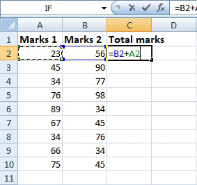
Step 1: We write the formula in any cell and press enter so that it is calculated. In this example, we write the formula(= B2 + A2) in cell C2 and press enter to calculate the formula.

Step 2: Now click on the Fill handle at the corner of cell which contains the formula(C2).

Step 3: Drag the Fill handle up to the cells you want to fill. In our example, we will drag it till cell C10.

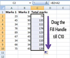
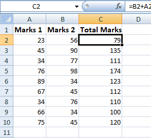
Step 4: Now we can see that the addition operation is performed between the cell A2 and B2, A3 and B3 and so on.

Step 5: You can double-click on any cell to check that the operation is performed in between which cells.

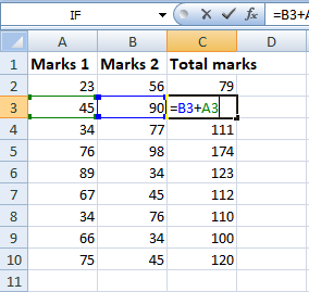
Thus, in the above example, we see that the relative address of cell A2 changes to A3, A4, and so on, similarly the relative address changes for column B, depending on the relative position of the row.

Absolute Reference

Absolute reference is the cell reference in which the row and column are made constant by adding the dollar ($) sign before the column name and row number. The absolute reference does not change as you copy the formula from one cell to other. If either the row or the column is made constant then it is known as a mixed reference. You can also press the F4 key to make any cell reference constant. $A$1, $B$3 are examples of absolute cell reference.

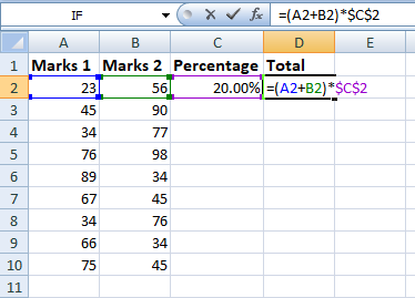
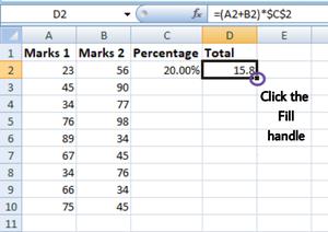
For example, We want to multiply the sum of marks of two subjects, entered in column A and column B, with the percentage entered in cell C2 and display the result in column D. Here, we will use absolute reference so that the address of cell C2 remains constant and does not change with the relative position of column and rows.

Steps to Use Absolute Reference:

Step 1: We write the formula in any cell and press enter so that it is calculated. In this example, we write the formula(=(A2+B2)*$C$2) in cell D2 and press enter to calculate the formula.

Step 2: Now click on the Fill handle at the corner of cell which contains the formula(D2).

Step 3: Drag the Fill handle up to the cells you want to fill. In our example, we will drag it till cell D10.

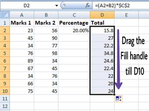
Step 4: Now we can see that the percentage is calculated in column D.

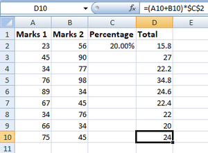
Step 5: You can double-click on any cell to check that the operation is performed in between which cells, and we see that the address of cell C2 does not change.

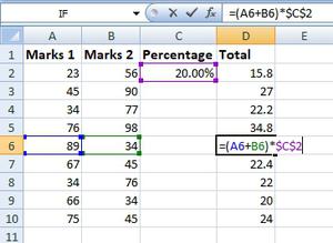
Thus, in the above example we see that the address of cell C2 is not changed whereas the address of column A and B changes with the relative position of the row and column, this happened because we used the absolute address of the cell C2.

Источник

Содержание

Switch between relative, absolute, and mixed references
Cell References in Excel – Relative, Absolute, Mixed
What is a Cell Reference?
For example:
Types of Cell Reference in Excel
1. Relative Cell Reference
How to Use Relative Cell References in Excel
#Example 1:
#Example 2:
When to Use Relative Cell References in Excel
2. Absolute Cell Reference
How to Use Absolute Cell References in Excel
#Example:
What Does the Dollar ($) Sign Do?
When to Use Absolute Cell References in Excel
3. Mixed Cell Reference
#Example:
Some Other Ways of Using Cell References With Examples
Relative and Absolute Cell References for Calculating Dates
Whole Column Reference
Whole Row Reference
Refer to an Entire Column, Excluding the First Few Rows
Using a Mixed Entire Column Reference in Excel
How to switch between Absolute, Relative, and Mixed References
Important Points to Remember
FAQs on Excel Cell References
1. What are the 3 types of cell references in Excel?
Relative and Absolute Cell References in MS Excel
Relative Reference
Absolute Reference

Switch between relative, absolute, and mixed references

As an example, if you copy the formula =B4*C4 from cell D4 to D5, the formula in D5 adjusts to the right by one column and becomes =B5*C5. If you want to maintain the original cell reference in this example when you copy it, you make the cell reference absolute by preceding the columns (B and C) and row (2) with a dollar sign ( $). Then, when you copy the formula =$B$4*$C$4 from D4 to D5, the formula stays exactly the same.

To change the type of cell reference:

Select the cell that contains the formula.

In the formula bar , select the reference that you want to change.

Press F4 to switch between the reference types.

The table below summarizes how a reference type updates if a formula containing the reference is copied two cells down and two cells to the right.

Источник

Cell References in Excel – Relative, Absolute, Mixed

Microsoft Excel, sometimes known as MS Excel, is a potent spreadsheet programme. In Excel, each worksheet consists of a number of cells that are made up of rows and columns. Each cell has a unique reference, which enables users to quickly access and address the required cell (or cells) within the functions. In Excel, cell references are crucial, particularly when working with huge data sets in functions and formulas.

This article covers a quick overview of Excel Cell References. The various sorts of cell references that Excel offers and the detailed instructions for using each one are also covered in the article.

What is a Cell Reference?

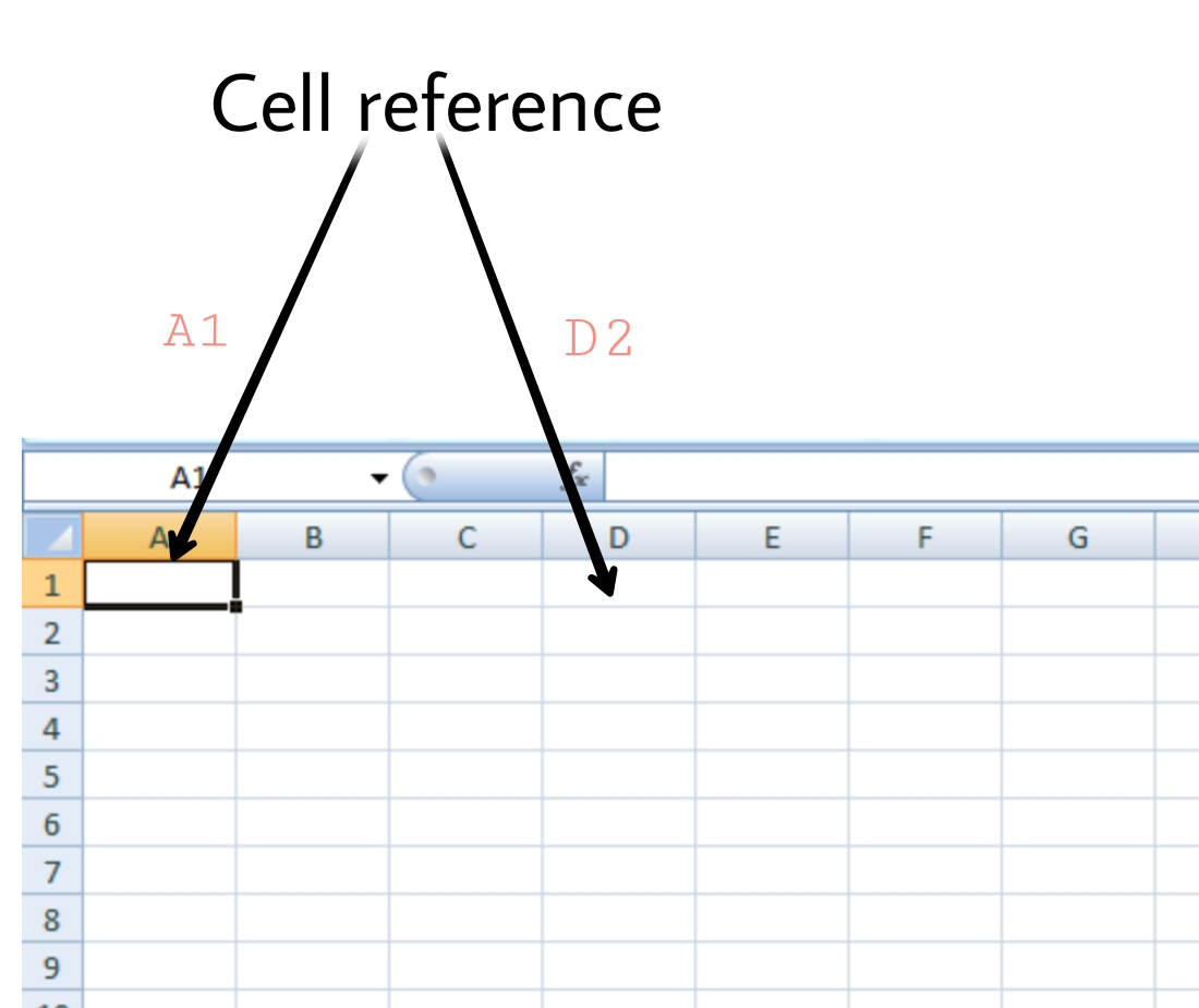
An Excel cell reference, also known as a cell address, is a mechanism that defines a cell on a worksheet by combining a column letter and a row number. We can refer to any cell (in Excel formulas) in the worksheet by using the cell references.

For example:

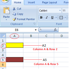
Here we refer to the cell in column A & row 2 by A2 & cell in column A & row 5 by A5. You can make use of such notations in any of the formulas or copy the value of one cell to another cell (by using = A2 or = A5).

Types of Cell Reference in Excel

Understanding various cell references primarily makes it easier for us to use Excel formulas and avoid unexpected formula errors. When copying and pasting Excel formulas, this is quite useful. Based on various use situations, Excel offers three main types of cell references, including:

Relative Cell Reference
Absolute Cell Reference
Mixed Cell Reference

1. Relative Cell Reference

In Excel, a relative cell reference is used by default. Excel uses a relative reference whenever we insert a cell reference or a range within a formula. The relative references, which commonly reflect the combination of column name and row number, are used normally with the associated cell references. There is no dollar ($) sign in the relative reference for the cell.

How to Use Relative Cell References in Excel

Let’s see how to use the Relative Cell references through examples,

#Example 1:

If you refer to cell B1 from cell E1, actually you would be referring to a cell that is 3 columns to the left (E-B = 3) within the same row number 1.

When it is copied to other locations present in a worksheet, the relative reference for that location will be changed automatically. (because relative cell reference describes offset to another cell rather than a fixed address as In our example, offset is : 3 columns left in the same row).

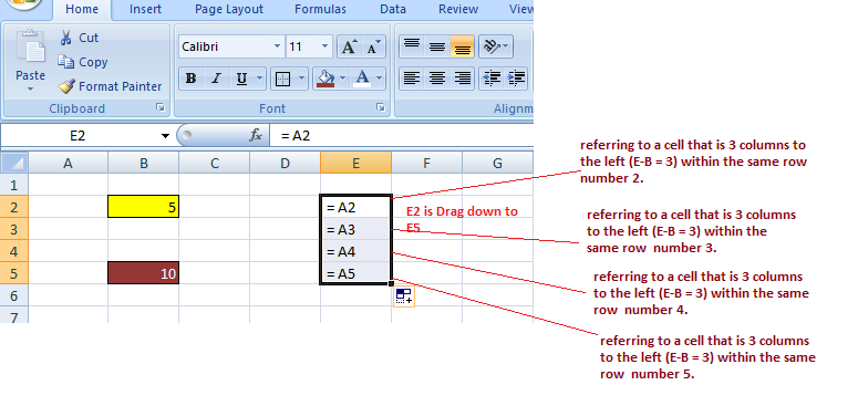
#Example 2:

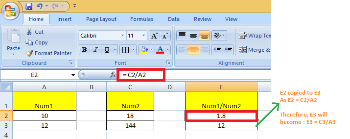
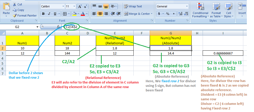
If you copy the formula = C2 / A2 from the cell “E2” to “E3”, the formula in E3 will automatically become =C3/A3.

When to Use Relative Cell References in Excel

When you need to develop a formula for a set of cells and the formula needs to make a reference to a relative cell reference, relative cell references come in handy.

When this occurs, you can create the formula in one cell and copy it before pasting it into every other cell.

2. Absolute Cell Reference

When copying or using AutoFill, there are times when the cell reference must stay the same. A column and/or row reference is kept constant using dollar signs. So, to get an absolute reference from a relative, we can use the dollar sign ($) characters.

To refer to an actual fixed location on a worksheet whenever copying is done, we use absolute reference. The reference here is locked such that rows and columns do not shift when copied.

How to Use Absolute Cell References in Excel

Below is an example depicting how to use Absolute Cell References in Excel.

#Example:

When we fix both row & column – Say if we want to lock row 2 & column A, we will use $A$2 as:

G2 = C2/$A$2, when copied to G3, G3 becomes = C3/$A$2

Note: C3 is 4 columns left to G3 in the same row.

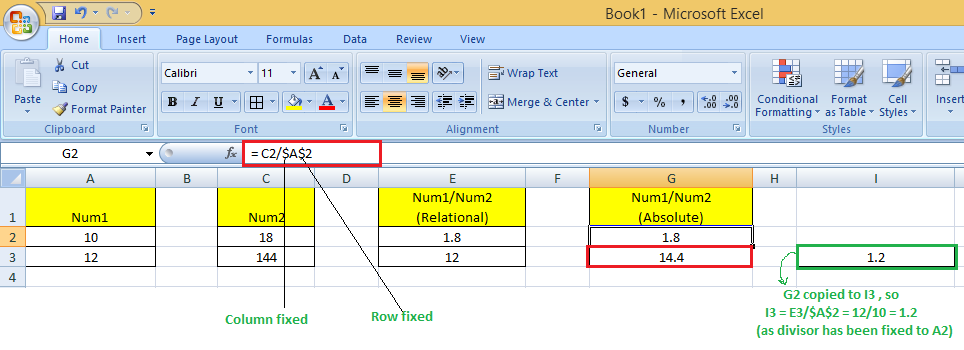
Here, original cell reference A2 is maintained whenever we copy G2 to any of the cells. So I3 = E3/$A$2 because E3 comes from the relative reference (4 columns left to the current one) & /$A$2 comes from the absolute reference.

Therefore, I3 = E3//$A$2 = 12/10 = 1.2

What Does the Dollar ($) Sign Do?

When the row and column numbers are preceded by the dollar symbol ($), it becomes absolute (i.e., stops the row and column number from changing when copied to other cells). Dollar ($) before the row fixes the row & before the column fixes the column.

When to Use Absolute Cell References in Excel

When you don’t want the cell reference to alter when you replicate formulas, absolute cell references come in handy. This can be the situation if you have to use a fixed value in the formula.

3. Mixed Cell Reference

An absolute column and relative row, or an absolute row and relative column, is a mixed cell reference. You get an absolute column or absolute row when you individually put the $ before the column letter or before the row number. Example: $B8 is relative to row 8 but absolute for column B, and B$8 is absolute for row 1 but relative for column A.

Here, the Dollar ($) before the row number fixes/locks the row & before the column name fixes/locks the column.

#Example:

When we fix the only row: If we have G2 = C2/A$2 then :

We used $ before the row number, so we are locking the only row here. When G2 is copied to G3, G3 = C3/A$2 (not C3/A3) because the row has been fixed already.

Here, whenever we copy G2 to any other cell, always the divisor will refer to a fixed row 2 (column vary according to the concept of relative reference)

So, when G2 is copied to I3, I3 = E3/C$2 because E3 comes from the relative reference (4 columns left to the current one) & C$2 comes from the absolute reference for row & relative reference for Column (6 Columns left to the current one)

Some Other Ways of Using Cell References With Examples

Now that we are familiar with the basics of using Cell References in Excel, let’s see some other ways of using cell references.

Relative and Absolute Cell References for Calculating Dates

We can use relative and absolute cell references to calculate dates.

Example: To Calculate the Date of Delivery online from the given date of the order placed & no of days it will take to deliver :

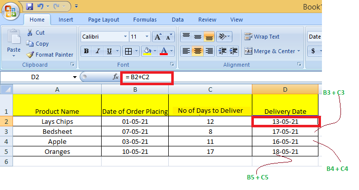
Here, We calculate the Date of Delivery by = Order Date + No of days to deliver. We used Relative cell reference so that individual product delivery dates can be calculated.

Absolute cell references for calculating dates :

Example: To Calculate the Date of Birth When the age is known is a number of days using Current date can be done by making use of absolute reference.

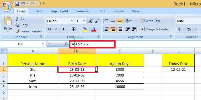
Here, We calculate DOB by = Current Date – Age in days. The Current date is contained in the cell E2 & in subtraction, we fixed that date to subtract from the days.

Whole Column Reference

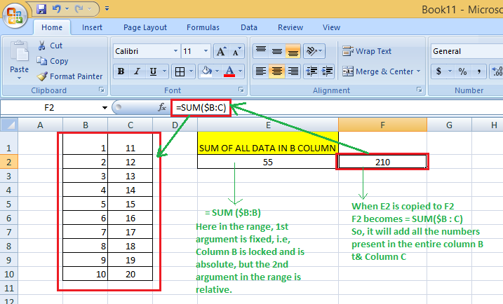
You will want to refer to all the cells inside a particular column when operating with an Excel worksheet with any number of rows. Simply type a column letter twice with a colon in between to refer to the entire column B, for example, B:B.

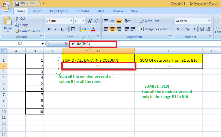
Example: You may want to find the sum of a column of data in certain cases. While you can do this with a regular cell range, such as =SUM(B1:B10), you will need to change the cell range if your spreadsheet grows in size.

Excel, on the other hand, has a cell range that does not require the row number and takes all the cells in the column in action. If you wanted to find the sum of all the values in column B, for example, you would type =SUM (B:B). You can add as much data as you want to your spreadsheet without having to change your cell ranges if you use this type of cell range.

Whole Row Reference

You will want to refer to all the cells inside a particular row when operating with an Excel worksheet with any number of columns. Simply type a row number twice with a colon in between to refer to the entire row, for example, 2:2.

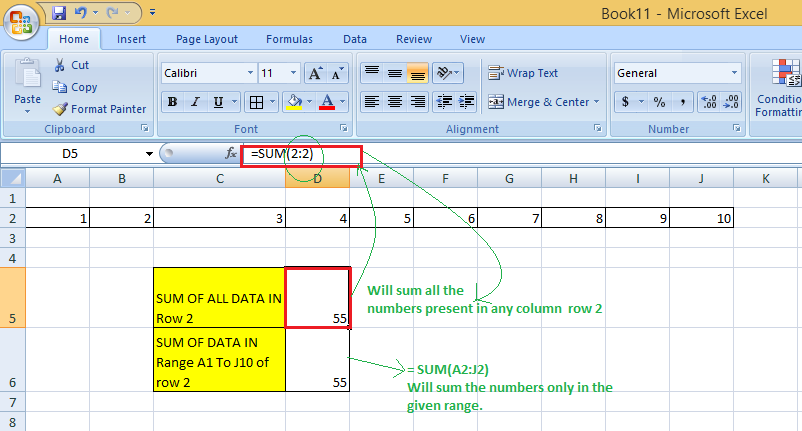
Example: You may want to find the sum of a row of data in certain cases. While you can do this with a regular cell range, such as =SUM(A2 : J2), you will need to change the cell range if your spreadsheet grows in size.

Excel, on the other hand, has a cell range that does not require the column letter and takes all the cells in the row in action. If you wanted to find the sum of all the values in row 2, for example, you would type =SUM (2:2). You can add as much data as you want to your spreadsheet without having to change your cell ranges if you use this type of cell range.

Refer to an Entire Column, Excluding the First Few Rows

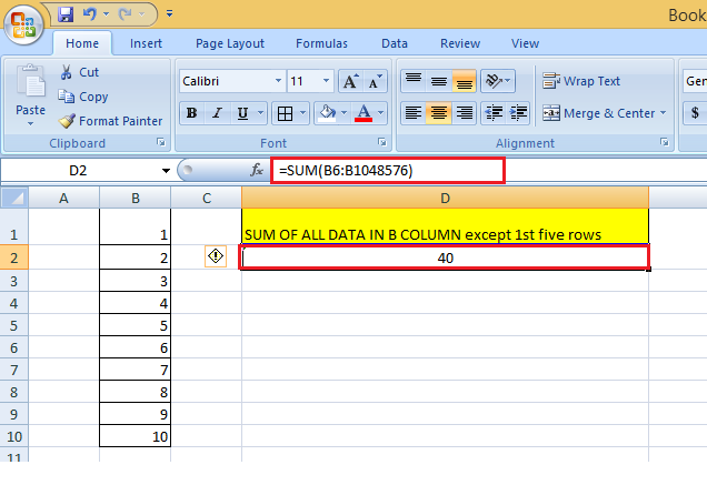
To refer to the entire column excluding the first few rows, you need to specify the range as we give in a normal fashion. We know that the Excel worksheets can have only 1,048,576 rows. (To check this, go to an empty cell & press: Ctrl + Down arrow Key)

So, we can do the sum of the entire column B except for the first 5 rows by = SUM(B6:B1048576).

Using a Mixed Entire Column Reference in Excel

You can also create a mixed entire-column reference, say for example $B:B. But, practically, it is difficult to find a situation where it would be used.

Example :

How to switch between Absolute, Relative, and Mixed References

The $ sign can be manually typed in an Excel formula to adjust a relative cell relation to absolute or mixed. You can also speed things up by pressing the F4 key. You must be in formula edit mode to use the F4 shortcut. The steps are :
Firstly, choose the cell that contains the formula. Then, by pressing the F2 key or double-clicking the cell, you can enter Edit mode. Select the cell reference in which you want to make changes. Then, switch between four-cell reference forms by pressing F4.

Example: When you select a cell having only relative reference (i.e., no $ sign), say = B2:

The first time when you press F4, it becomes =$B$2
The second time when you press F4, it becomes =B$2
The third time when you press F4, it becomes=$B2
The fourth time when you press F4, it becomes back to the relative reference=B2

B2 –Press F4–> =$B$2 –Press F4–> =B$2 –Press F4–> = =$B2 –Press F4–> =B2

So, using F4, you do not require to manually type the $ symbol.

Important Points to Remember

One of the crucial components for Excel functions or formulas is the cell reference.

Excel formulas that employ relative cell references automatically change the references to match the correct row and column.

When copying formulas into non-relative cells, absolute cell references are advised. Excel keeps the absolute cell references constant.

According to the specifications, a mixed reference only locks one of the references, either the row or the column. Not both are locked.

FAQs on Excel Cell References

1. What are the 3 types of cell references in Excel?

Ans: In Excel, we can use one of three types of cell references:

Relative Cell References
Absolute Cell References
Mixed Cell References

Источник

Relative and Absolute Cell References in MS Excel

Referencing the cell of other worksheets is known as External referencing.
Referencing the cell of other programs is known as Remote referencing.

There are two types of cell references in Excel:

Relative reference
Absolute reference

Relative Reference

Steps to Use Relative Reference:

Step 1: We write the formula in any cell and press enter so that it is calculated. In this example, we write the formula(= B2 + A2) in cell C2 and press enter to calculate the formula.

Step 2: Now click on the Fill handle at the corner of cell which contains the formula(C2).

Step 3: Drag the Fill handle up to the cells you want to fill. In our example, we will drag it till cell C10.

Step 4: Now we can see that the addition operation is performed between the cell A2 and B2, A3 and B3 and so on.

Step 5: You can double-click on any cell to check that the operation is performed in between which cells.

Absolute Reference

Steps to Use Absolute Reference:

Step 1: We write the formula in any cell and press enter so that it is calculated. In this example, we write the formula(=(A2+B2)*$C$2) in cell D2 and press enter to calculate the formula.

Step 2: Now click on the Fill handle at the corner of cell which contains the formula(D2).

Step 3: Drag the Fill handle up to the cells you want to fill. In our example, we will drag it till cell D10.

Step 4: Now we can see that the percentage is calculated in column D.

Step 5: You can double-click on any cell to check that the operation is performed in between which cells, and we see that the address of cell C2 does not change.

Источник

Workbooks and worksheets

Excel works with files called workbooks. Each workbook contains one or more spreadsheets, called worksheets. Each worksheet consists of cells organized in a rectangular grid. The rows of a worksheet are labeled with a number and the columns are labeled with a letter or series of letters. The first row is labeled 1, the next 2, and so on. The first column is labeled A, the next B, etc. The column after Z is labeled AA, and then AB, AC, and so on. The column after AZ is BA, and then BB, BC, etc. The column after ZZ is AAA, and then AAB, AAC, etc.

Figure 1 – Sample Excel Worksheet

Each worksheet can contain up to 1,048,578 rows and 16,384 columns (i.e. column A through XFD).

Cell values, addresses and ranges

You can enter any of the following into a cell:

A number (e.g. 45 or -23.006)
Text (e.g. London)
A truth value (TRUE or FALSE)
A formula (e.g. =SUM(A4:B7)/4)

Numeric values can also appear in scientific notation: e.g. the value 4.5E-05 is equivalent to .000045 (i.e. 4.5 with the decimal point moved 5 places to the left) and 4.5E+05 is equivalent to 450000 (i.e. 4.5 with the decimal point moved 5 places to the right).

If you want Excel to treat a number as text then you need to precede the number with a single quote – e.g. ‘4.5 is considered to be the text 4.5.

Cell references

Each cell also has an address, consisting of a row and a column label. E.g., in Figure 1 the cell with address A5 contains the text “London”, while the cell with address C6 contains the number 8.1.

You can also reference a range of cells. For our purposes, we only consider rectangular ranges, which consist of a rectangular collection of cells. Such ranges are specified as two cell addresses separated by a colon. E.g. the range C5:C10 consists of the 5 cells from cell C5 to C10, which for Figure 1 corresponds to the data elements for Brand B. The range A4:D10 consists of all the cells in the rectangle whose opposite corners are A4 and D10, which for Figure 2.1 corresponds to all the data in the table, including row and column headings, but excluding totals.

A cell reference consists of an address of a single cell (e.g. G17 or AB8) or of a cell range (e.g. A1:D6 or ZZ1:AAB14). Cell references can also be named. E.g. you can highlight the range B5:D5 in the worksheet in Figure 1, right-click and select Define Name … to assign the name London to the range B5:D5.

Cell selection

The usual way of selecting a cell is to simply move the mouse pointer to that cell and left-click. To select a range of cells, click on a cell in one of the four corners of that range and then highlight the remaining cells in the range using the mouse. If the cells you want to select are not visible you can use the horizontal and vertical scroll bars in the usual manner to make the desired cell range visible.

Increasing cell width

If the contents of a cell are too big for the space allocated to that cell you may see the contents displayed as #######. To properly see the real contents you may need to increase the width of the column containing this cell.

E.g. suppose cell B5 is not wide enough for its contents. You can increase the width of column B by moving the mouse pointer to the vertical line at the border between the headers for column B and column C (the column to the right of B). Once it is in the correct position the mouse pointer changes shape; now hold down the left mouse button and move the mouse pointer to the right to increase the column width (or left to decrease the column width). You can also change the width of a column by right-clicking on the column heading and selecting the Column Width… option.

Formulas

As mentioned above, besides numbers and text, cells can contain formulas. Formulas are built up from the following components preceded by the equal symbol (=):

Numbers
Text
Operators
Cell references
Worksheet functions

Operators include the following:

Arithmetic operators: addition (+), subtraction (-), multiplication (*), division (/) and exponentiation (^)
The concatenation operator: & (used to concatenate text)
Logical comparison operators: less than (<), greater than (>), less than or equal (<=), greater than or equal (>=), equal (=) and not equal (<>)

Precedence rules

The usual precedence rules apply, namely multiplication and division are applied before addition and subtraction, and exponentiation is applied before any of the other operators. Parentheses are used to change the order in which operators are applied. For example:

4+5*2 = 14 (4+5)*2 = 18

3^2-1 = 8 3^(2-1) = 3

-(3^2)+1 = -8 (-3)^2+1 = 10

For some reason, Excel violates the usual precedence rules by giving a unary minus sign precedence over exponentiation. E.g. Excel calculates -3^2+1 as if it were (-3)^2+1 and so returns a value of 10 instead of -8. Similarly, -1^2 is evaluated as 1 instead of -1. To get the correct answer you need to use the expression -(1^2).

Excel provides a variety of worksheet functions such as SUM, MIN, LOG, etc. We will describe these in more detail shortly.

Cell values

Each cell has a value. For cells containing a number, text, or truth value, the value of the cell is simply the contents of the cell. For cells containing a formula, the value is the evaluation of the formula based on the values of any referenced cells. Some examples of the values of formulas are given in Figure 2.

Figure 2 – Values of Excel Formulas

In the example in Figure 1, notice that cell B11 contains the formula =SUM(B5:B10). The value of this formula, and therefore the value of cell B11, is 106.1. This is the value that is actually displayed in the cell. The formula is displayed in the Formula Bar, just above the grid, to the right of the symbol f_x.

Note too that if we had assigned the name BrandA to the range B5:B10, then the formula =SUM(BrandA) would be equivalent to =SUM(B5:B10) and would have the same value.

Specifying a formula

In specifying a formula such as =A1+3 you can simply type the formula character by character. Alternatively, you can type the character = and click on the A1 cell and then continue by typing +3. Excel will automatically specify the correct formula. Similarly, for a formula that contains a cell range such as =SUM(A1:B4) you can type =SUM( and highlight the cell range A1:B4 and then type the right parenthesis to complete the formula.

Error values

If a cell has an illegal value you will see an error value displayed in the cell. E.g., if you enter =A1/0 into cell B1 then cell B1 will have the value #DIV/0 indicating that you are attempting to divide by zero. These error values all start with the symbol # and include #DIV/0, #N/A, #NUM!, #VALUE!, #NAME?, #NULL! and #REF!

Observations

One of the things that gives Excel such power is that when you change the value of any cell then the value of all formulas that reference that cell also change. E.g., if you change the value of cell B5 in the worksheet in Figure 1 from 23.5 to 13.5 then the value of cell B11 will automatically change from 106.1 to 96.1.

You can copy the contents of any cell into another cell (or, in fact, any cell range into another cell range, usually of the same size and shape). If the content of the first cell is a number, text or truth value, then the second cell will contain the same number, text, or truth value. When the contents of the first cell is a formula then the second cell will also contain a formula, but the specific formula depends on the type of addressing that is used.

Relative and absolute addressing

Excel provides two types of addressing when defining a cell or cell range: absolute and relative addressing. The default is relative addressing. For example, the contents of cell B11 in the worksheet in Figure 1 is =SUM(B5:B10). Here B5:B10 is a relative address. If this formula is copied into cell D11, then D11 will contain the formula =SUM(D5:D10), which accomplishes the same function as the formula in cell B11, namely to sum the values in the 5 cells above it, and so the value of cell D11 will be 43.3.

The usual way of copying the contents of one cell into another is to click on the first cell (B11 in the example above), press Ctrl-C (copy), and then click on the second cell (D11 in the example above) and press Ctrl-V (paste).

The dollar symbol $ is used to specify absolute addressing. When copying a formula that contains a dollar sign to another cell location, any part of an address that contains a $ does not change. E.g., suppose cell B11 in the worksheet from Figure 1 contains the formula =SUM($B$5:$B$10). Its value is still the same, namely 106.1, but this time when we copy the contents of cell B11 into D11, then D11 will also contain the formula =SUM($B$5:$B$10), and so the value of cell D11 will be 106.1 and not 43.3.

Note that we can use absolute addressing on any part of a cell address, namely, B11 (no absolute addressing), B$11 (absolute addressing for the row, but relative addressing for the column), $B11 (absolute addressing for the column, but relative addressing for the row) and $B$11 (absolute addressing for both row and column).

Changing addressing type

To change from relative addressing (the default) to absolute addressing, you simply put the $ symbol in the appropriate place. Alternatively, you can highlight the cell address in the Formula Bar or in the cell itself and press the function key F4. E.g. if you highlight the cell reference A3 and press the F4 key, then A3 changes to $A$3. If you press F4 again it changes to A$3. Pressing F4 again changes the reference to $A3, and finally pressing F4 one more time returns the cell address to the original reference of A3.

Cell references to a different worksheet

You can also reference cells in another worksheet. To do this you need to precede the reference (absolute or relative) by the name of the worksheet followed by !. The default names for worksheets in Excel are Sheet1, Sheet2, etc., although these names can be changed as explained below. Thus the (relative) reference to range A3:B4 in Sheet1 is Sheet1!A3:B4. You don’t really need to worry about all of this since by clicking on a cell in another worksheet, Excel automatically copies the correct reference address into the formula.

References

Walkenbach, J. (2010) Microsoft Office Excel 2010 Bible. Wiley.

GCF Global (2022) Excel formulas
https://edu.gcfglobal.org/en/excelformulas/

Источник

Чем отличается абсолютная, относительная и смешанная адресация

Важность ссылки на ячейки Excel трудно переоценить. Ссылка включает в себя адрес, из которого вы хотите получить информацию. При этом используются два основных вида адресации – абсолютная и относительная. Они могут применяться в разных комбинациях и различными способами, что создает различные виды ссылок.

Если вы будете понимать разницу между абсолютными, относительными и смешанными ссылками, то вы на полпути к освоению мощи и универсальности формул и функций Excel. И вот о чем мы должны поговорить:

Абсолютная адресация
Относительная адресация
Смешанная адресация
Как можно изменить тип адреса?

Применение абсолютной адресации.

Абсолютная – это адресация, при которой идёт указание на конкретную ячейку, адрес которой не изменяется.

Все вы, наверное, видели знак доллара ($) в формулах Excel и задавались вопросом, что это такое. $ — признак абсолютной адресации. Знак $ может стоять в двух местах – перед буквой столбца и перед номером строки.

Действительно, вы можете ссылаться на одну и ту же ячейку четырьмя разными способами, например A1, $A$1, $A1 и A$1.

Знак доллара в ссылке влияет только на одно – он указывает Excel, как обрабатывать этот адрес, когда формула перемещается или копируется в таблице. То есть, использование знака $ перед координатами строки и столбца создает абсолютную ссылку, которая не изменится при копировании или перемещении. Без знака $ ссылка будет относительной и будет меняться, если вы будете копировать или переносить данные в новое место.

Абсолютная адресация в Excel предназначена для того, чтобы можно было многократно использовать одни и те же значения в таблицах, не вводя из каждый раз. Или сделать какой-то расчет единожды и использовать его результаты многократно. При этом вы можете изменять вашу таблицу, добавляя в нее новые ячейки, строки и столбцы, либо перемещая уже существующие на новое место. Ваши формулы и ссылки не «поломаются».

Абсолютная адресация может быть полезна для самых различных расчетов, чтобы сделать их более эффективными. Вот несколько возможностей, о которых следует помнить:

Вы можете использовать фиксированную цену товара или услуги, фиксированную налоговую ставку в ваших расчётах.
Сделайте вычисления один раз и используйте этот результат многократно в других таблицах.
Используйте одни и те же значения в счетах-фактурах или заказах на поставку.

Абсолютная адресация ячеек нам может быть нужна в том случае, когда мы копируем формулу, одна часть которой состоит из переменной величины (например, стоимость товара), а вторая имеет постоянное значение (скажем, размер скидки). То есть, у нас есть постоянная константа, с которой нужно многократно провести определенную операцию (умножение, деление, вычисление процента и т.д.).

Вводим выражение =B2*$F$2 в С2. Таким образом мы при помощи умножения найдём сумму скидки по первому товару.

Нажмите и, удерживая левую кнопку мыши, перетащите маркер автозаполнения насколько необходимо вниз. В нашем случае это диапазон С2:С8. Отпустите кнопку мыши. Формула будет скопирована в выбранные ячейки с абсолютной ссылкой. И в каждой будет вычислен результат.

В нашем примере мы применили абсолютную адресацию – $F$2. Как видите, при копировании вниз по столбцу адрес этот не изменился.

Основной способ использования абсолютного адреса – это создание теми или иными способами абсолютной ссылки. Как мы уже говорили выше, это делается путем применения в адресе знака доллара $. Он позволяет зафиксировать вертикальные или горизонтальные координаты, либо и те, и другие одновременно.

Знак $ можно ввести вручную. Для этого нужно установить курсор перед первым значением координат адреса (по горизонтали), находящегося в ячейке или в строке формул. Далее, в англоязычной раскладке клавиатуры следует нажать на клавиатуре цифру «4» в верхнем регистре (при этом удерживая клавишу Shift). Именно там расположен символ доллара. Затем нужно то же действие проделать и с координатами по вертикали.

Существует и более быстрый способ. Нужно установить курсор в ячейку, в которой находится адрес, и нажать функциональную клавишу F4. После этого знак доллара моментально появится дважды: одновременно перед координатами по горизонтали и вертикали данного адреса. Многократное нажатие F4 позволит получить разные варианты расположения $ в ссылке – в зависимости от того, что вы хотите зафиксировать.

Еще один способ применить абсолютную адресацию – дать ячейке имя. Для этого установите курсор на нужную клетку таблицы и в поле «Имя» впишите ее новое название. Далее вы можете использовать его в ваших расчётах. Важным достоинством этого подхода является и то, что теперь разбираться в ваших вычислениях стало намного проще.

Здесь важно помнить, что в имени можно использовать только буквы и цифры. Если очень хочется присвоить имя, состоящее из нескольких слов, поставьте между ними нижнее подчёркивание (_).

Вот как это может выглядеть на самом простом примере. Вместо «скидка» в любой формуле в этом файле будет использоваться содержимое F2.

Альтернативный и не такой удобный способ именования — это использовать меню. Выбираем Вставка, Имя, Присвоить. Появляется окно, в него вводим имя, нажимаем Добавить и ОК.

И, наконец, есть еще третий способ создать абсолютную адресацию ячейки.

Решение заключается в использовании функции ДВССЫЛ(), которая из текстового значения создает ссылку. Если записать такое выражение:

=ДВССЫЛ(«A2»),

то оно всегда будет указывать на адрес A2 вне зависимости от любых дальнейших действий, вставки или удаления столбцов и т.д.

Небольшая сложность состоит в том, что если целевая ячейка A2 пуста, то ДВССЫЛ возвратит ноль, что не всегда удобно. Однако, это можно легко обойти, используя чуть более сложную конструкцию с проверкой через функцию ЕПУСТО():

=ЕСЛИ(ЕПУСТО(ДВССЫЛ(«A2″));»»;ДВССЫЛ(«A2»))

Ну а чем же отличается абсолютная адресация от относительной?

Применение относительной адресации.

Относительную адресацию применять очень просто, так как именно она используется в Excel по умолчанию. То есть, когда вы создаете ссылку, она всегда будет относительной. Относительная адресация означает, что при копировании или перемещении ссылки на какое-то количество строк или столбцов соответствующим образом будут изменяться и координаты относительно первоначального расположения.

То есть, новые координаты изменяются относительно текущего расположения ячейки с формулой.

Рассмотрим на примере.

=A1*B1 – данную формулу, записанную в С1, Excel читает следующим образом: содержимое клетки, находящейся на два столбца слева в той же строке, нужно перемножить с содержимым ячейки, находящейся на один столбец слева в той же строке.

Если это выражение скопировать из С1 в С2, то его понимание для Excel остается точно таким же. То есть, он возьмет ячейку, находящуюся на 2 столбца слева от текущих координат (теперь это будет A2), и перемножит ее с той, которая находится на один столбец слева (то есть, B2).

И формула в С2 примет вид =A2*B2

Если скопировать в С3, то она изменится на =A3*B3.

Когда по умолчанию в вашей формуле использована относительная адресация, то при копировании вниз по столбцу у входящих в нее адресов ячеек номер строки будет увеличиваться.

Ежели копировать формулу вправо, то буква столбца будет увеличиваться по алфавиту. А если влево, то буква столбца будет уменьшаться.

Относительная адресация нужна, если для однотипных данных в строке или столбце выполнить одинаковые вычисления. Например, для нескольких товаров количество умножить на цену.

В этом случае мы записываем формулу один раз (как правило, в верхнюю или самую левую позицию), а затем цепляем мышкой маркер автозаполнения и протаскиваем куда необходимо. Всё пространство заполняется автоматически.

Смешанная адресация.

Если нужно, чтобы при перемещениях адрес изменялся не полностью, применяют так называемую смешанную адресацию.

Смешанная – это адресация, при которой идёт изменение только одной координаты. Знак $ ставится только в одном месте: или перед буквой столбца или перед номером строки. В зависимости от этого и происходят изменения.

Например, в адресе $A5 при копировании вниз и вверх номер строки будет меняться, а при тиражировании вправо и влево имя столбца меняться не будет.

Или в адресе A$5 при копировании вниз и вверх по столбцу номер строки не будет изменяться, а при передвижении вправо и влево имя столбца будет меняться.

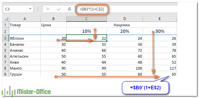
Предположим, нам нужно определить цену товара при различных уровнях наценки. Как это сделать максимально быстро? Вот тут нам и пригодится смешанная адресация.

Формула в С3 будет такая:

=$B3*(1+C$2)

Это означает, что в первом сомножителе мы всегда адресуемся к столбцу B. Но номера строк могут меняться в зависимости от расположения формулы.

Во втором сомножителе нам всегда нужна строка 2, в которой записаны проценты надбавки. А вот столбец может изменяться.

Единожды записав эту формулу в B3, копируем ее по строке вправо до E5. И тут же, не снимая выделения, тащим мышкой маркер заполнения в E9. В результате формулу мы ввели единожды, а таблица вся заполнена!

Таким образом, грамотное применение адресации может сэкономить массу времени.

Как изменить тип адресации?

Проще всего это сделать, если она организована при помощи знака $.

В этом случае откройте ячейку на редактирование, кликнув по ней мышкой либо нажав F2. Затем установите курсор на нужный адрес и несколько раз нажмите на F4. С каждым нажатием расположение знаков $ будет изменяться, пока не появится нужный вам вариант.

Ну или можно расставить $ руками в нужных местах.

В следующих статьях мы подробно разберем, как наиболее правильно и рационально использовать разные типы адресации при создании ссылок и написании формул.

Как удалить сразу несколько гиперссылок — В этой короткой статье я покажу вам, как можно быстро удалить сразу все нежелательные гиперссылки с рабочего листа Excel и предотвратить их появление в будущем. Решение работает во всех версиях Excel,…

Как использовать функцию ГИПЕРССЫЛКА — В статье объясняются основы функции ГИПЕРССЫЛКА в Excel и приводятся несколько советов и примеров формул для ее наиболее эффективного использования. Существует множество способов создать гиперссылку в Excel. Чтобы сделать ссылку на…

Гиперссылка в Excel: как сделать, изменить, удалить — В статье разъясняется, как сделать гиперссылку в Excel, используя 3 разных метода. Вы узнаете, как вставлять, изменять и удалять гиперссылки на рабочих листах, а также исправлять неработающие ссылки. Гиперссылки широко используются…

Как использовать функцию ДВССЫЛ – примеры формул — В этой статье объясняется синтаксис функции ДВССЫЛ, основные способы ее использования и приводится ряд примеров формул, демонстрирующих использование ДВССЫЛ в Excel. В Microsoft Excel существует множество функций, некоторые из которых…

Как сделать диаграмму Ганта — Думаю, каждый пользователь Excel знает, что такое диаграмма и как ее создать. Однако один вид графиков остается достаточно сложным для многих — это диаграмма Ганта. В этом кратком руководстве я постараюсь показать…

Как сделать автозаполнение в Excel — В этой статье рассматривается функция автозаполнения Excel. Вы узнаете, как заполнять ряды чисел, дат и других данных, создавать и использовать настраиваемые списки в Excel. Эта статья также позволяет вам убедиться, что вы…

Быстрое удаление пустых столбцов в Excel — В этом руководстве вы узнаете, как можно легко удалить пустые столбцы в Excel с помощью макроса, формулы и даже простым нажатием кнопки. Как бы банально это ни звучало, удаление пустых…

Источник

Содержание

Определение абсолютных и относительных ссылок
Пример относительной ссылки
Ошибка в относительной ссылке
Создание абсолютной ссылки
Смешанные ссылки
Вопросы и ответы

При работе с формулами в программе Microsoft Excel пользователям приходится оперировать ссылками на другие ячейки, расположенные в документе. Но, не каждый пользователь знает, что эти ссылки бывают двух видов: абсолютные и относительные. Давайте выясним, чем они отличаются между собой, и как создать ссылку нужного вида.

Определение абсолютных и относительных ссылок

Что же представляют собой абсолютные и относительные ссылки в Экселе?

Абсолютные ссылки – это ссылки, при копировании которых координаты ячеек не изменяются, находятся в зафиксированном состоянии. В относительных ссылках координаты ячеек изменяются при копировании, относительно других ячеек листа.

Пример относительной ссылки

Покажем, как это работает на примере. Возьмем таблицу, которая содержит количество и цену различных наименований продуктов. Нам нужно посчитать стоимость.

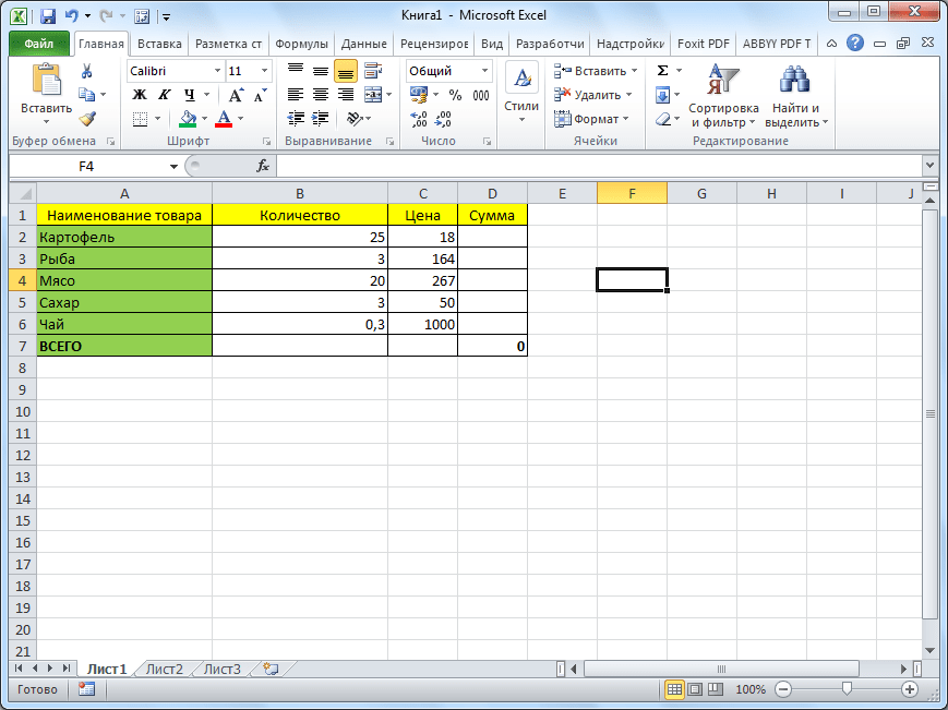
Делается это простым умножением количества (столбец B) на цену (столбец C). Например, для первого наименования товара формула будет выглядеть так «=B2*C2». Вписываем её в соответствующую ячейку таблицы.

Теперь, чтобы вручную не вбивать формулы для ячеек, которые расположены ниже, просто копируем данную формулу на весь столбец. Становимся на нижний правый край ячейки с формулой, кликаем левой кнопкой мыши, и при зажатой кнопке тянем мышку вниз. Таким образом, формула скопируется и в другие ячейки таблицы.

Но, как видим, формула в нижней ячейке уже выглядит не «=B2*C2», а «=B3*C3». Соответственно, изменились и те формулы, которые расположены ниже. Вот таким свойством изменения при копировании и обладают относительные ссылки.

Ошибка в относительной ссылке

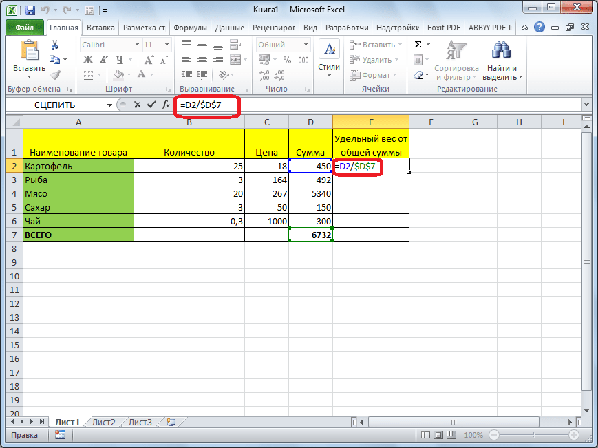
Но, далеко не во всех случаях нам нужны именно относительные ссылки. Например, нам нужно в той же таблице рассчитать удельный вес стоимости каждого наименования товара от общей суммы. Это делается путем деления стоимости на общую сумму. Например, чтобы рассчитать удельный вес картофеля, мы его стоимость (D2) делим на общую сумму (D7). Получаем следующую формулу: «=D2/D7».

В случае, если мы попытаемся скопировать формулу в другие строки тем же способом, что и предыдущий раз, то получим совершенно неудовлетворяющий нас результат. Как видим, уже во второй строке таблицы формула имеет вид «=D3/D8», то есть сдвинулась не только ссылка на ячейку с суммой по строке, но и ссылка на ячейку, отвечающую за общий итог.

D8 – это совершенно пустая ячейка, поэтому формула и выдаёт ошибку. Соответственно, формула в строке ниже будет ссылаться на ячейку D9, и т.д. Нам же нужно, чтобы при копировании постоянно сохранялась ссылка на ячейку D7, где расположен итог общей суммы, а такое свойство имеют как раз абсолютные ссылки.

Создание абсолютной ссылки

Таким образом, для нашего примера делитель должен быть относительной ссылкой, и изменяться в каждой строке таблицы, а делимое должно быть абсолютной ссылкой, которая постоянно ссылается на одну ячейку.

С созданием относительных ссылок у пользователей проблем не будет, так как все ссылки в Microsoft Excel по умолчанию являются относительными. А вот, если нужно сделать абсолютную ссылку, придется применить один приём.

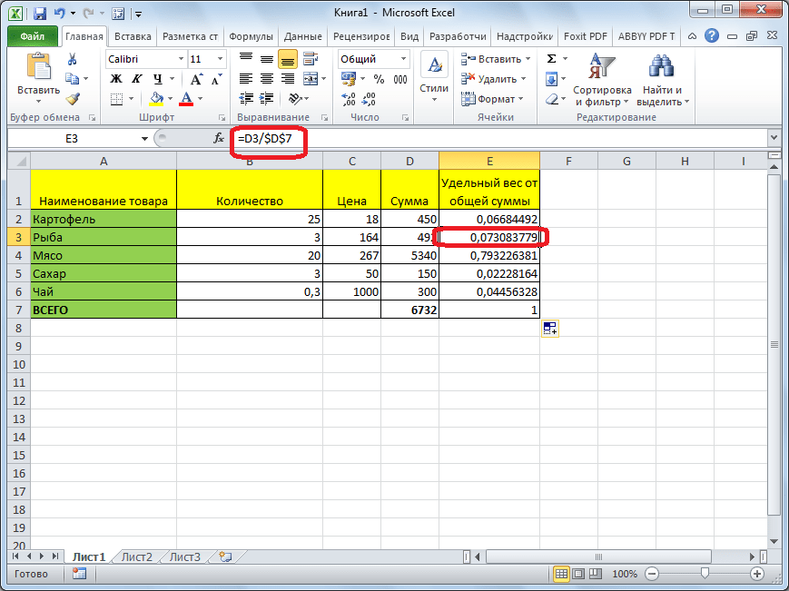
После того, как формула введена, просто ставим в ячейке, или в строке формул, перед координатами столбца и строки ячейки, на которую нужно сделать абсолютную ссылку, знак доллара. Можно также, сразу после ввода адреса нажать функциональную клавишу F7, и знаки доллара перед координатами строки и столбца отобразятся автоматически. Формула в самой верхней ячейке примет такой вид: «=D2/$D$7».

Копируем формулу вниз по столбцу. Как видим, на этот раз все получилось. В ячейках находятся корректные значения. Например, во второй строке таблицы формула выглядит, как «=D3/$D$7», то есть делитель поменялся, а делимое осталось неизменным.

Смешанные ссылки

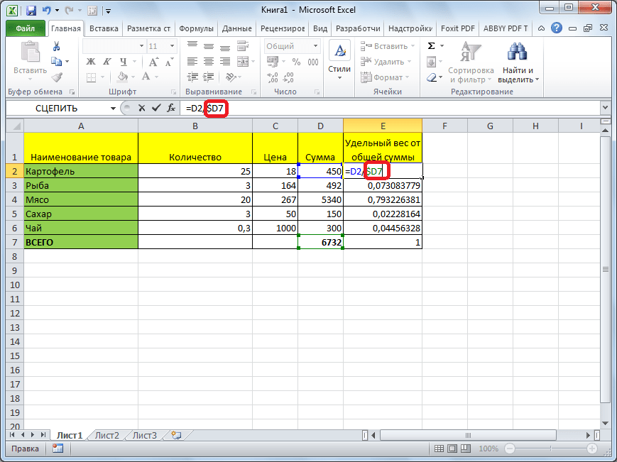
Кроме типичных абсолютных и относительных ссылок, существуют так называемые смешанные ссылки. В них одна из составляющих изменяется, а вторая фиксированная. Например, у смешанной ссылки $D7 строчка изменяется, а столбец фиксированный. У ссылки D$7, наоборот, изменяется столбец, но строчка имеет абсолютное значение.

Как видим, при работе с формулами в программе Microsoft Excel для выполнения различных задач приходится работать как с относительными, так и с абсолютными ссылками. В некоторых случаях используются также смешанные ссылки. Поэтому, пользователь даже среднего уровня должен четко понимать разницу между ними, и уметь пользоваться этими инструментами.

Источник

Absolute and relative addresses in Excel. Relative addresses are addresses that change when copying a formula. This is the default address when we formulate the formula. For example A1, B2 … The absolute address is the one that was not changed when copying the formula. The absolute address is distinguished from the absolute address with the character $. For example $ A1 $ 1, $ B1 $ 2….

What is relative and absolute address and how to identify it?

Relative addresses are addresses that change when copying a formula. This is the default address when we formulate the formula. For example A1, B2 .

The absolute address is that the address you did not change when copying the formula. The absolute address is distinguished from the absolute address with the character $. For example $ A1 $ 1, $ B1 $ 2….

Mixed addresses are a combination of relative and absolute addresses. For example $ A1. B $ 2….

For example, relative and absolute address differentiation:

With the formula of column F3 = VLOOKUP (D3, $ I $ 2: $ J $ 5,2, FALSE).

Address D3 is the relative address. And $ I $ 2: $ J $ 5 is the absolute address. When you copy the formula to cell D4, the formula in D4 will be = VLOOKUP (D4, $ I $ 2: $ J $ 5,2, FALSE).

When copying the formula, Excel changed the position D3 => D4 corresponding to the change correlated with the position of cells F3 and F4. The position of the region $ I $ 2: $ J $ 5 is preserved because you have set it to the absolute position.

Ways to convert relative and absolute references

Relative addresses are the default addresses when you formulate. To switch to the relative position you press the F4 button immediately after entering the relative position.

For example, in any cell you type: = B1, you press 1 key F4 => address changes to = $ B $ 1: absolute for both columns and rows). You press once again F4 => address changes to = B $ 1: absolute line and relative column. Next press F4 => the address changes to = $ B1: relative row and absolute column. You press the F4 key to return to the absolute address = B1.

Apply relative and absolute addresses in Excel

The absolute wall address is applied in the LOOKUP, INDEX, MATCH, search functions SUMIF, COUNTIF, RANK, etc. that need to extract data from related tables.

Example of using the RANK function to rank a series of numbers:

With the above usage, you leave the Value value as a relative value so that when copying the formula changes according to the position of the cell that returns the result. As for the array $ G $ 3: $ G $ 12 you leave the absolute value to not change position when copying the formula.

Above Dexterity Software has introduced readers with absolute and relative address. Hope the article will help you. Good luck!!!

Источник

July 28, 2012

Excel, Technology

The most important concept that you must master in Excel is Relative and Absolute Addressing. This is the basic foundation of Excel. Without understanding this, you will not work with excel with ease.

Formula Philosophy:

Excel is defaulted to Relative Addressing!
Relative Addressing is when you copy a formula across and it increments the letters in the formula.
Relative Addressing is when you copy a formula down and it increments the numbers in the formula.
The formula does change but it does not have to do what column or row you are sitting at. It is irrelevant.
Excel’s job is to zoom into the formula based on how you are copying/filling (across or down), it will do exactly what is told to do. Letters across and numbers down.
For example: =Sum(F20:F40) Copying across will increment the letter “F” to “G”.
For example: =Sum (B2:F2) Coping down will increment the row “2” to “3”.
Absolute Addressing is opposite of Relative Addressing. You want to lock in the cell in a formula so that when you copy across or down the particular cell does not change. It is absolutely locked. Place the Insert beam in the formula before, in the middle or after the cell that needs to be locked. Hit F4 key. This will place a $ signs next to the letter and row number. For example , if you need the value in G2 and it must be used for all the rows, then you must lock it. Excel does not tell you that it has to be locked. For example, G2 is the cell I want to use, it should look like this: $G$2.

F4 has four different absolute set up.
- Hitting F4 the 1^st time Excel places both dollar signs – $G$2
- Hitting F4 a 2^nd times Excel places a dollar sign in front of the number – G$2
- Hitting F4 a 3^rd time Excel places a dollar sign in front of the letter – $G2
- Hitting F4 a 4^th time Excel keeps the original letter and number – G2

Why would I want to use Absolute? The reason is that if you have a bonus of 15% in a cell and the salaries are going to be multiplied by 15%, then I will write a formula that uses the salaries times the bonus rate that is located in the cell. I would not type the following formulas:
- =B2*15%
- =B3*15%
- =B4*15% and so on.
  This does not work because if you decide to change the 15% to 20% then you have to retype the formula and copy it down. If the formula is very large, you may make other typing mistakes.
- Remember, Excel works for you!

Here is an example of an Excel sheet with name, salary, bonus amount, and total salary. 15% is in G2

Place 15% percent in the cell G2. Then type in C3:
=B2*G2 and while the insert beam is blinking, hit F4 the formula now become
=B2*$G$2 hit Enter
Copy the formula and the rest is typed in for you leaving G2 intact.
=B3*$G$2
=B4*$G$2

For your information, if you did not place the absolute in G2, when you copy down, Excel zooms into the formula and it is told to increment the row numbers. Therefore, B3 becomes B4 which then becomes B5 and G2 will become G3 which then becomes G4. The last 2 formulas will produce a zero values become something times nothing gives you ZERO!

Pressing Ctrl+` keys (` is located to the left of the number 1 key) shows you the formulas. Pressing those two keys will return back to normal view. It is an On/Off switch.

Practice makes perfect and Absolute is used everywhere in Excel. You can not hide from this concept!

**Click on the example to see it better.

Источник