Relational database and excel

Excel used to be the poor schmuck’s database, with spreadsheets that just sort of sat there. You could create something more sophisticated with LOOKUP functions, but they were a huge hassle to set up.

Not anymore: Excel 2013’s table tools include features that make it easy to link charts and cells, perform searches, and create dynamically updated reports, just like—yes—a relational database. Excel can handle a lot of day-to-day office data this way, and we’ll show you how to set it up.

How Excel makes a relational database

Relational databases—databases structured to recognize relations among the information stored in them—are essential for working with large amounts of business data. They let you quickly search and retrieve specific information, view the same data set in multiple ways, and reduce data errors and redundancy. Try doing that with a spreadsheet.

To show you how Excel makes it easier, we will create two tables: the master table and the detail table. The master table is the primary table, which generally contains unique records (such as name, address, city, state, etc.). This table rarely changes except to, say, add or delete individuals.

For every record in the master table, there can be many records in the detail tables (also called slave or child tables) that link back to the master table. This is called a one-to-many relationship. The data in the detail tables—such as daily sales, product prices, quantities—usually changes constantly.

To avoid repeating all the master information in every detail table, you create relationships using one unique field, such as the Sales ID, then let Excel do the rest. For example, you have 10 sales people who all have unique, demographic information (master table). Each sales person has 200 products that he/she sells (detail or child table). At the end of each year, you need a report that provides the total yearly sales by person, but you also need a report that provides the total sales by city.

For this tutorial, we’ll create a master table with the salespersons’ information and a second table that provides their total sales, by quarter, for the year. The Sales ID is the relational field that connects the tables. Then, we’ll create a report (or pivot table) that shows which cities had the highest sales.

Open Excel and select a new, blank worksheet.

Create the master table

1. First, double-click the tab at the bottom of the screen (above the green bar line) and type Master over the tag line Sheet1.

2. In cell A1 type: Master. In cells A3 through F3 type these column headers: Sales ID, Sales Person, Address, City, State, Zip Code.

3. In cells A4 through A13 type the sales ID numbers—in this case, 101 through 110. The Sales ID is the unique data value that’s used to create a relationship between your two tables.

4. Enter names, addresses, cities, states, and zip codes in the remaining cells. You can copy the information from this sample worksheet or create your own data. Since we are looking for the highest sales by city, be sure to create multiple cities in your table. For example, we have three salespeople in Los Angeles, two in Hollywood, two in San Francisco, and three in San Diego.

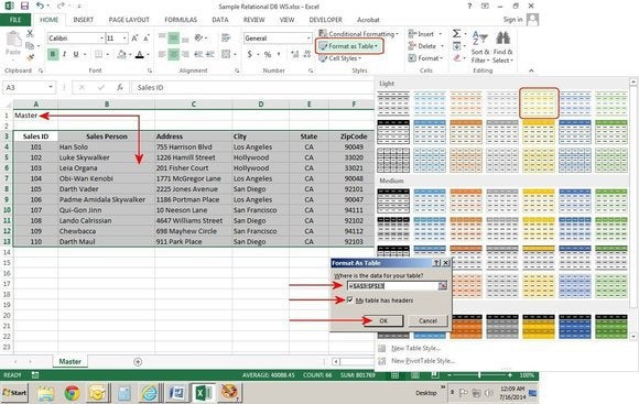
5. Once the data is entered, highlight A3 through F13, including the column headers. From the Styles group, select Format as Table. From the dropdown, choose a color and format you like. A Format As Table dialog box appears with the table range displayed in the white box. Ensure that the My Table Has Headers box is checked, then click OK.

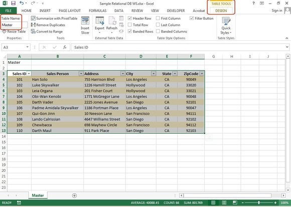
6. With the table still highlighted, select the Design tab under the text that says Table Tools (this option is available only when the table is highlighted). In the Properties group (far left), in the box under Table Name, type Master.

Create the detail table

1. At the bottom of the screen beside the Master tab, click the ‘+’ sign to insert a new sheet. Double-click the tab and type Sales over the tag line Sheet2.

2. In cell A1, type Total Sales for 2013. In cells A3 through E3, type Sales ID, Quarter1, Quarter2, Quarter3, and Quarter4.

3. In cells A4 through A13 type the sales ID numbers: 101 through 110.

4. In B4 through E13, enter 40 random numbers that represent sales dollars or copy the data from this example table.

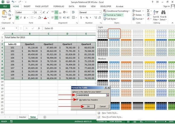
5. Once the data is entered, highlight cells A3 through E13. From the Styles group, select Format as Table. From the dropdown, choose a color and format you like. A Format As Table dialog box appears with the table range displayed in the white box. Ensure that the My Table Has Headers box is checked, then click OK.

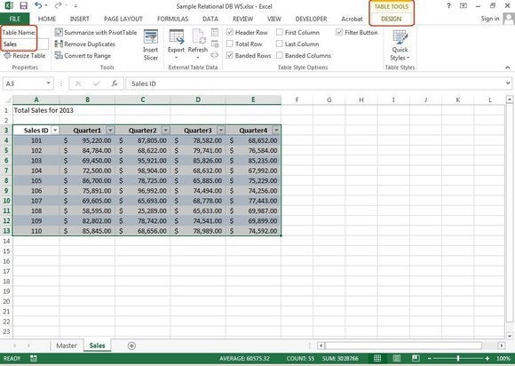
6. With the table still highlighted, select the Design tab under the text that says Table Tools (this option is only available when the table is highlighted). In the Properties group, in the box under Table Name, type Sales.

Set relationships in the pivot table report section

The first rule of pivot tables: You must define the table relationships within the Pivot Table report section. Do not attempt to create the relational connections first, because Excel will not recognize them from the Pivot Table reporting section. Also, be sure to select the detail table (Sales) for the “analyze data” table, otherwise it won’t work.

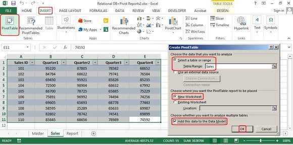
1. Go to the Sales table and highlight cells A1 through E11. Click the Insert tab, then click the Pivot Table button.

2. In the Create Pivot Table dialog box, ensure that the Select a Table or Range > Table Range field says “Sales.” If you want to import a table/database from another program such as Word or Access, click the second option, Use an External Data Source.

3. In the second field—Choose Where You Want the Pivot Report placed—click New Worksheet if you want the table on a separate sheet by itself, or click Existing Worksheet if you want the report to drop in beside your Sales table.

4. And for the last field—Choose Whether You Want to Analyze Multiple Tables—click Add this Data to the Data Model, then click OK.

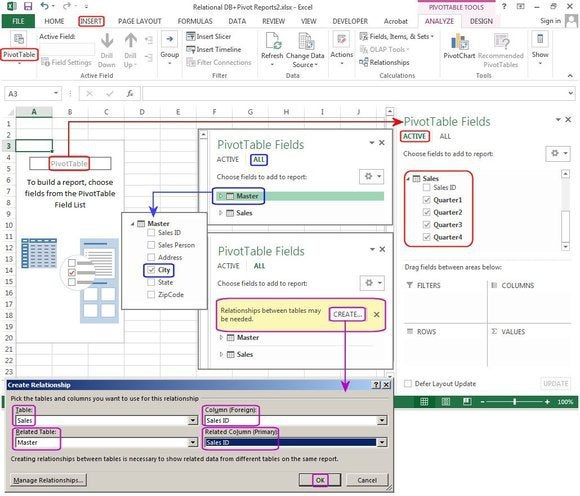
The Pivot Table menus appear with a Help box on the left that says “To build a report, choose fields from the Pivot Table field list.”

1. Under Pivot Table Fields, the Active button is selected because only one table is currently active. Click the boxes Quarter1, Quarter2, Quarter3, and Quarter4 and some numbers appear in a grid on the left.

2. Click the All button, then click the Master table link. The fields from the Master table appear. Click the box beside City. A yellow box appears that says “Relationships between tables may be needed.”

3. This is where you define the relationship between the two tables. Click the Create button and the Create Relationship dialog box appears. Under Table, click the down arrow and choose Sales from the available tables list. Under Column (Foreign), click the arrow and choose Sales ID from the field list.

4. Remember the Sales ID is the only field that’s in both tables. Under Related Table, choose Master and under Related Column (Primary), choose Sales ID again, then click OK.

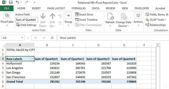
Excel makes the connection, then displays the report on the screen: Total Sales by City. Enter a report title in A1, and it’s complete.

Sort, create filters, and select data by other fields

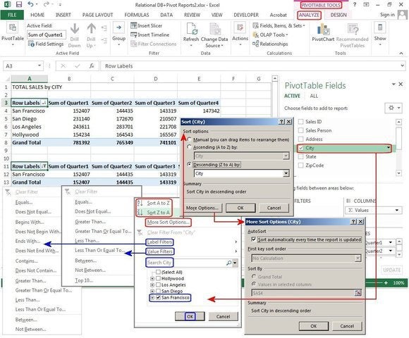
Filters are used to select specific data by fields. To filter the data by city, click anywhere inside the table, then click the city field—notice the small arrow on the right.

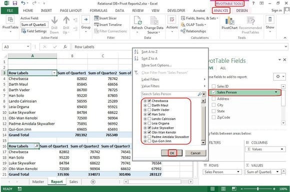
1. Click the arrow and the Sort-Filter Options dialog box pops up with selections for Filters and Sorting. If you want to Sort, click Sort A to Z or Sort Z to A, or see the graphic below for the options under Sort More Options.

The Filter options include Label Filters, Value Filters, and Search (or select specified records in the current search field). If you have a huge database with hundreds of records, you can enter a city name (or partial name) in the Search box, then click the hour glass to locate the specified record/city. Excel displays the city in the list below the Search box.

2. If your database is relatively small, first uncheck the Select All button, then scroll down to the city you want, click the box, then click OK. The report now shows total sales for each quarter in that city only.

Label Filters and Value Filters are additional filtering options to help you refine your search. For example, in the Label Filters, if you choose all cities that Begin With “S,” you get San Diego and San Francisco. If you choose all cities Less Than “S,” you get Hollywood and Los Angeles. Numeric fields are filtered the same way most all other databases do it—Less Than, Greater Than, Equals, Between, etc.

3. You can also select a different field and quickly create a new report. For example, if you’d like to see the quarterly sales plus totals by sales person, uncheck City and check Sales Person. The report drops in.

4. Next, click Sales Person, click the down arrow, then uncheck Select All in the Sort-Filter Options dialog box. Click four names on the list, click OK, and the filtered report drops in.

The Pivot Tables/database options are endless. There are numerous ways to analyze the data, create and manage sets, group fields, insert slicers and timelines, drill up and down, and import and export data, as well as design reports with custom layouts and styles, create hundreds of colorful charts, then print it all out for distribution.

Charts and styles

To spice up your table before you print it, try adding a chart and/or some colors and style to the table.

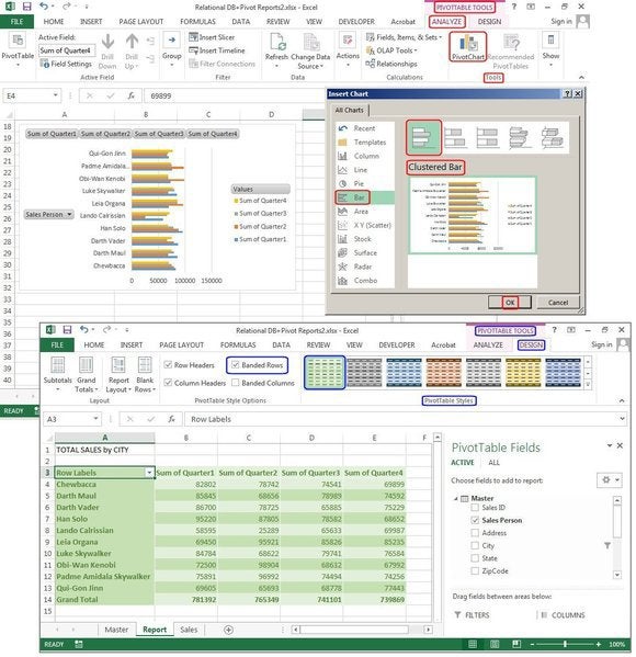
To add a chart, highlight the table, select Pivot Table Tools > Analyze > Tools > Pivot Chart, then select a chart from the gallery of charts, and click OK.

To add colors and style, select Pivot Table Tools > Design > Pivot Table Styles and choose a table design from the gallery of styles. Click Banded Rows under the Pivot Table Style Options group to alternate colors and/or shading on the odd and even rows for easier viewing. And that’s all there is to it.

With this new relational database/table feature, this process is so easy that once it’s set up in Excel, you can extract specific data and create dozens of reports in minutes.

When a full RDBMS is overkill, you can use Excel to model relational data over multiple spreadsheets. Simple but surprisingly powerful!

Anyone who works with databases appreciates the value of raw data—the colours, borders and other embellishments people add to spreadsheets are redundant fluff that detracts from the data’s value. We like strings, integers, floats, dates and other basic datatypes in spreadsheets and we don’t like it when people insert rows that serve as headings because they’ll be lost when the data is sorted or filtered.

Bad table

Type	Value
Foo	Bar
	Baz
Foo2	Bar2
	Baz2

Good table

Type	Value
Foo	Bar
Foo	Baz
Foo2	Bar2
Foo2	Baz2

What is VLOOKUP?

And herein lies the problem: if you’re repeating values in attempt to make a spreadsheet more data-oriented and less report-like you’ve denormalized the data by repeating values. Enter VLOOKUP.

VLOOKUP is short for “Vertical Lookup” and is used for tables with headings in the first row (whereas if headings were in the first column you’d use HLOOKUP) and it’s syntax is as follows:

=VLOOKUP(4, Clients!A:Z, 2, 0)

Parameters:

1. Lookup value: can be a value or a cell reference
2. Lookup table: logical table in which to search—in this case, another sheet
3. Column offset: number of columns from the search column to be returned
4. Range lookup: 0/false for exact match, 1/true for sheer madness first value less than or equal to the lookup value

Usage example

1. Create a new spreadsheet
2. Create two sheets called People and Cars
3. In the People sheet:
   1. Create two column headings called ID and Name
   2. Enter test data, e.g. 1: Rich, 2: Chris, 3: Jim
4. In the Cars sheet:
   1. Create two column headings called Car and Owner
   2. Enter test data in first column, e.g. Beamer, Lambo, Jag
   3. In cell B2, enter =VLOOKUP(3, People!A:B, 2, 0)
   4. In cell B3, enter =VLOOKUP(2, People!A:B, 2, 0)
   5. In cell B4, enter =VLOOKUP(1, People!A:B, 2, 0)

What just happened?!

What you’re now looking at is the value of a cell in another sheet based on the ID for its row. This allows you to use the spreadsheet like a relational database without having to store the same data in multiple places and it’s completely human-readable, so (provided people don’t start messing with vlookups) even non-technical people can use it.

Conclusion

VLOOKUP allows basic data modelling within a spreadsheet using one file per database and one sheet per table. It certainly can’t take over from a full RDBMS but for simple data (especially data that must be available to non-technical people) it’s certainly a useful tool to be aware of.

Try using this technique for managing Clients with many Projects, or for Sales and Customers for your small business or even as an accounting system with income, outgoings, clients, invoices, etc.

This site uses cookies to give you the best experience. By clicking “Accept All”, you consent to the use of ALL the cookies. However, you may visit «Cookie Settings» to provide a controlled consent.

You must have used MS Excel for tasks like preparing reports, forecasts, and budgets. But do you know Excel is much powerful than this.  As, in Excel you can make a searchable database.

Want to learn how to create searchable database in Excel? don’t worry this post will guide you to make a database in Excel.

Well if we talk about Excel database capabilities than no doubt it is very powerful. Besides of creating simple searchable database in Excel you can also it for making relational database in Excel.

So, let’s take a complete overview on how to create database in Excel whether it’s searchable or relational?

What’s The Need Or Benefits Of Making Database In Excel?

Excel Spreadsheets are mainly designed for evaluating the data and sort listing the items, for short term storage of raw data. Overall, spreadsheet is used for crunching numbers and for storing single list of items. So, it is the best application for keeping inventory, computing data and statistical data modeling.

But when it comes to store large amount of data it’s best to use a database in Excel. Database suits best for circumstances where more than two user needs to share their information.

Apart from this, the two most important benefits of database in Excel are:

• Reduced data redundancy
• It will raise the capacity of data integrity
• Reduced updating errors and increased consistency
• Greater data integrity and independence from applications programs
• You can easily maintain report and share your data
• Improved data security
• Reduced data entry, storage, and retrieval costs

Just follow down the steps mentioned below to create a searchable database Excel.

Step 1: Entering the data

In a database, columns are called as fields. So, as per your need you can add as many fields you need.

In the shown example, database fields are StdID, StdName, State, Age, Department, and Class Teacher.

Now you can enter data into this newly creating database easily. Each time you enter a new data it will get fill-up in the first empty row after the Fields.

Like this,

So, you can also see how easy it is to enter data into an Excel database.

Step 2: Entering Data Correctly

While entering data into the Excel database, don’t leave any row or column empty. As it is strictly prohibited.

It’s a clear breakdown of your Excel database. actually, the reason behind this is. As soon as Excel finds a completely blank column/row. It doesn’t count that column or row in the database.

So, if you left any row or column in your database completely empty then it will divide your database into different parts. Whatever functions you apply to your database will not work for that disconnected piece of information.

Although it is allowed to leave some cells of row to be empty. Like this:

Step 3: Know that the Rows are called Records

Each single row of database is known as records. so, you can see here all the rows are records.

Step 4: Know that the Columns are called Fields

All the headings of the database columns are termed as Field Names.

So here in the shown figure, database field name are: StdID, StdName, State, Age, Department, and Class Teacher.

Note:

Try to format field names other than the rows of the database. Table field names are organized with different styles other than table’s cell.

Step 5: Creating the Table

For making table in your database, just choose for any cell in the data range. After then in the insert tab make a click on the table command.

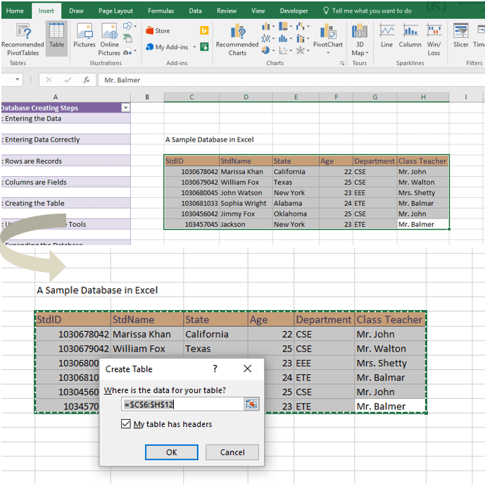
Clicking on the table will open a Create Table dialog box. Tap to the ok option and it create a table.

For filtering out the data, make use of the drop-down arrows which is appearing on the heading of each column.

Step 6: Using the Database Tools

Well for the proper data analysis and interpretation in excel database you can make use of database tools. For learning more about such tools click here.

Step 7: Expanding the Database

Now everything set up, so you can start adding more records and fields in your database.

Step 8: Completing the Database Formatting

At last you just have do formatting of the database columns. There are many tools to do cells formatting in the database. Like you can make use of the cell styles, within the drop down “Format As Table”. You can also work with the commands present in the format cells dialog box.

That’s all, you have created a searchable database in your Excel spreadsheet.  Now it’s time to learn how to use this Searchable Database In Excel.

How To Use A Searchable Database In Excel?

Use Excel’s Lookup functions to search a database

by using the Excel Lookup functions, one can easily design a worksheet which enable you to search any database table.

Suppose, you have imported following table from your Access database into sheet 2 of the Excel workbook.

To make an Excel worksheet which can be used to check intern’s pay scale just by providing intern’s ID. Here are the following steps to perform:

1. Open your Excel workbook, tap on the Sheet2 tab, and choose the range A2:H5.
2. Now hit on the Name box and type Interndata. After then press [Enter].
3. Tap on the Sheet1 tab.
4. Select the cell D6 and put Employee ID.
5. Choose the cell D8 and assign Name.
6. Select the cell E8 and put the following function:

=VLOOKUP(E6,Interndata,3,FALSE)&” “&VLOOKUP(E6,Interndata,2,FALSE)

1. In the D10 enter the Pay Rate.
2. Now tap to the E10 and enter the following function:

=VLOOKUP(E6,Interndata,8,FALSE)

1. It’s time to change the cell format of E6, E8, and E10 for matching the data type with the data present in table.
2. Now add a header and do formatting as done and shown here.

How Does A Relational Database Work In Excel?

Excel is designed in such a way that it can smoothly work with the database. When the database items are associated, they make a record within multiple records’ group. Each Single record could be equivalent of row in spreadsheet. The hard to ignore the connection.

For creating a relational database in Excel, you have to join a master spreadsheet with slave spreadsheet or tables.

So, all an all, a relational database is having a master table which links with its slave tables, that are named as child tables.

Wrap up:

So, now you know it’s not that difficult task to make a searchable database in Excel. by performing the above steps, you can easily make a functional database which can be used for adding records. It can also be used to search for specific values in existing records by making use of the filter function.

Well this Excel database works smoothly for numbers of records. But the application performance starts degrading down after the accumulation of thousand of records.

Do you need to create and use a database? This post is going to show you how to make a database in Microsoft Excel.

Excel is the most common data tool used in businesses and personal productivity across the world.

Since Excel is so widely used and available, it tends to get used frequently to store and manage data as a makeshift database. This is especially true with small businesses since there is no budget or expertise available for more suitable tools.

This post will show you what a database is and the best practices you should follow if you’re going to try and use Excel as a database.

Get the example files used in this post with the above link and follow along below!

What is a Database?

A database is a structured set of data that is often in an electronic format and is used to organize, store. and retrieve data.

For example, a database might be used to store customer names, addresses, orders, and product information.

Databases often have key features that make them an ideal place to store your data.

Database vs Excel

An Excel spreadsheet is not a database, but it does have a lot of great and easy-to-use features for working with data.

Here are some of the key features of a database and how they compare to an Excel file.

Feature	Database	Excel
Create, read, update, and delete records	✔️	✔️ Excel allows anyone to add or edit data. This can be viewed as a negative consideration.
Data types	✔️	⚠️ Excel allows for simple data types such as text, numbers, dates, boolean, images, and error values. But lacks more complex data types such as date and timezones, files, or JSON.
Data validation	✔️	⚠️ Excel has some data validation features, but you can only apply one rule at a time and these can easily be overridden on purpose or by accident.
Access and security	✔️	❌ Excel doesn’t have any access or security controls. This is usually managed through your on-premise network or through SharePoint online. But anyone can access your Excel file if it’s downloaded and sent to them.
Version control	✔️	❌ Excel has no version control. This can be managed through SharePoint.
Backups	✔️	❌ Excel has no automated backups. These can be manually created or automated in SharePoint.
Extract and query data	✔️	✔️ Excel allows you to extract and query data through Power Query which is easy to learn and use.
Perform calculations	✔️	✔️ Excel has a large library of functions that can be used in calculated columns inside tables. Excel also has the DAX formula language for calculated columns in Power Pivot.
Aggregate and summarize data	✔️	✔️ Excel can easily aggregate and summarize data with formulas, pivot tables, or power pivots.
Relationships	✔️	✔️ Excel has many lookup functions such as XLOOKUP, as well as table merge functionality in Power Query, and 1 to many relationships in Power Pivot.
Scale with large amounts of data	✔️	⚠️ Excel can hold up to 1,048,576 rows of data in a single sheet. Tools like Power Query and Power Pivot can help you deal with larger amounts of data but they will be constrained based on your hardware specifications.
User friendly	❌ A database might not be user-friendly and may come with a steep learning curve that your intended users won’t be able to handle.	✔️ Most people have some experience with using Excel.
Cost	❌ Can be expensive to set up, run, and maintain a proper database tool.	✔️ Your organization might already have access to and use Excel.

This is not a comprehensive list of features that a database will have, but they are some of the major features that will usually make a proper database a more suitable option.

The features that a database has depends on what database it is. Not all databases have the same features and functionality.

You will need to decide what features are essential for your situation in order to decide if you should use Excel or some other database tool.

💡 Tip: If you have Excel for Microsoft 365, then consider using Dataverse for Teams as your database instead of Excel. Dataverse has many of the great database features mentioned above and it is included in your Microsoft 365 license at no additional cost.

Relational Database Design

A good deal of thought should happen about the structure of your database before you begin to build it. This can save you a lot of headaches later on.

Most databases have a relational design. This means the database contains many related tables instead of one table that contains all the data.

Suppose you want to track orders in your database.

One option is to create a single flat table that contains all the information about the order, the products, and the customer that created the order.

This isn’t very efficient as you end up creating multiple entries of the same customer information such as name, email, and address. You can see in the above data, column G, H, and I contains a lot of duplicate values.

A better option is to create separate tables to store the Order, Product, and Customer data.

The Order data can then reference a unique identifier in the Product and Customer data that will relate the tables and avoid unnecessary duplicate data entry.

This same example data might look like this when reorganized into multiple related tables.

1. An Orders table that contains the Item and Customer ID field.
2. A Products table that relates to the Item fields in the Orders table.
3. A Customers table that relates to the Customer ID in the Orders table.

This avoids duplicated data entry in a flat single table structure and you can use the Item or Customer ID unique identifier to look up the related data in the respective Products or Customers tables.

Tabular Data Structure in Excel

If you’re going to use Excel as your database, then you’re going to need your data in tabular format. This refers to the way the data is structured.

The above example shows a product order dataset in tabular format. A tabular data format is best suited for Excel due to the row and column structure of a spreadsheet.

Here are a few rules your data should follow so that it’s in tabular format.

• 1st row should contain column headings. This is just a short and descriptive name for the data contained below.
• No blank column headings. Every column of data should have a name.
• No blank columns or blank rows. Blank values within a field are ok, but columns or rows that are entirely blank should be removed.
• No subtotals or grand totals within the data.
• One row should represent exactly one record of data.
• One column should contain exactly one type of data.

In the above orders example data, you can see B2:E2 contains the column headings of an Order ID, Customer ID, Order Date, Item, and Quantity.

The dataset has no blank rows or columns, and no subtotals are included.

Each row in the dataset represents an order for one type of product.

You’ll also notice each column contains one type of data. For example, the Item column only contains information on the name of the product and does not include other product information such as the price.

⚠️ Warning: If you don’t adhere to this type of structure for your data, then summarizing and analyzing your data will be more difficult later. Tools such as pivot tables require tabular data!

Use Excel Tables to Store Data

Excel has a feature that is specifically for storing your tabular data.

An Excel Table is a container for your tabular datasets. They help keep all the same data together in one object with many other benefits.

💡 Tip: Check out this post to learn more about all the amazing features of Excel Tables.

You will definitely want to use a table to store and organize any data table that will be a part of your dataset.

How to Create an Excel Table

Follow these steps to create a table from an existing set of data.

1. Select any cell inside your dataset.
2. Go to the Insert tab in the ribbon.
3. Select the Table command.

This will open the Create Table menu where you will be able to select the range containing your data.

When you select a cell inside your data before using the Table command, Excel will guess the full range of your dataset.

You will see a green dash line surrounding your data which indicates the range selected in the Create Table menu. You can click on the selector button to the right of the range input to adjust this range if needed.

1. Check the My table has headers option.
2. Press the OK button.

📝 Note: The My table has headers option needs to be checked if the first row in your dataset contains column headings. Otherwise, Excel will create a table with generic column heading titles.

Your Excel data will now be inside a table! You will immediately see that it’s inside a table as Excel will apply some default format which will make the table range very obvious.

💡 Tip: You can choose from a variety of format options for your table from the Table Design tab in the Table Styles section.

The next thing you will want to do with your table is to give it a sensible name. The table name will be used to reference the table in formulas and other tools, so giving it a short descriptive name will help you later when reading formulas.

1. Go to the Table Design tab.
2. Click on the Table Name input box.
3. Type your new table name.
4. Press the Enter key to accept the new name.

Each table in your database will need to be in a separate table, so you will need to repeat the above process for each.

How to Add New Data to Your Table

You will likely need to add new records to your database. This means you will need to add new rows to your tables.

Adding rows to an Excel table is very easy and you can do it a few different ways.

You can add new rows to your table from the right-click menu.

1. Select a cell inside your table.
2. Right-click on the cell.
3. Select Insert from the menu.
4. Select Table Rows Above from the submenu.

This will insert a new blank row directly above the selected cells in your table.

You can add a blank row to the bottom of your table with the Tab key.

1. Place the active cell cursor in the lower right cell of the table.
2. Press the Tab key.

A new blank row will be added to the bottom of the table.

But the easiest way to add new data to a table is to type directly below the table. Data entered directly underneath the table is automatically absorbed into the table!

Excel Workbook Layout

If you are going to create an Excel database, then you should keep it simple.

Your Excel database file should contain only the data and nothing else. This means any reports, analysis, data visualization, or other work related to the data should be done in another Excel file.

Your Excel database file should only be used for adding, editing, or deleting the data stored in the file. This will help decrease the chance of accidentally changing your data, as the only reason to open the file will be to intentionally change the data.

Each table in the database should be stored in a separate worksheet and nothing else except the table should be in that sheet. You can then name the worksheet based on the table it contains so your file is easy to navigate.

💡 Tip: Place your table starting in cell A1 and then hide the remaining columns. This way it is clear the sheet should only contain the table and nothing else.

The only other sheet you might optionally include is a table of contents to help organize the file. This is where you can list each table along with the fields it contains and a description of what these fields are.

💡 Tip: You can hyperlink the table name listed in the table of contents to its associated sheet. Select the name and press Ctrl + K to create a hyperlink. This can help you navigate the workbook when you have a lot of tables in your database.

Use Data Validation to Prevent Invalid Data

Data validation is a very important feature for any database. This allows you to ensure only specific types of data are allowed in a column.

You might create data validation rules such as.

• Only positive whole numbers are entered in a quantity column.
• Only certain product names are allowed in the product column.
• A column can’t contain any duplicate values.
• Dates are between two given dates.

Excel’s data validation tools will help you ensure the data entered in your database follow such rules.

Follow these steps to add a data validation rule to any column in your table.

1. Left-click on the column heading to select the entire column.

When you hover the mouse cursor over the top of your column heading in a table, the cursor will change to a black downward pointing arrow. Left-click and the entire column will be selected.

The data validation will automatically propagate to any new rows added to the table.

1. Go to the Data tab.
2. Click on the Data Validation command.

This will open up the Data Validation menu where you will be able to choose from various validation settings. If there is no active validation in the cell, you should see the Any values option selected in the Allow criteria.

Only Allow Positive Whole Number Values

Follow these steps from the Data Validation menu to allow only positive whole number values to be entered.

1. Go to the Settings tab in the Data Validation menu.
2. Select the Whole number option from the Allow dropdown.
3. Select the greater than option from the Data dropdown.
4. Enter 0 in the Minimum input box.
5. Press the OK button.

💡 Tip: Keep the Ignore blank option checked if you want to allow blank cells in the column.

This will apply the validation rule to the column and when a user tries to enter any number other than 1, 2, 3, etc… they will be warned the data is invalid.

Only Allow Items from a List

Selecting items from a dropdown list is a great way to avoid incorrect text input such as customer or product names.

Follow these steps from the Data Validation menu to create a dropdown list for selecting text values in a column.

1. Go to the Settings tab in the Data Validation menu.
2. Select the List option from the Allow dropdown.
3. Check the In-cell dropdown option.
4. Add the list of items to the Source input.
5. Press the OK button.

📝 Note: If you place the list of possible options inside an Excel Table and select the full column for the Source reference, then the range reference will update as you add items to the table.

Now when you select a cell in the column you will see a dropdown list handle on the right of the cell. Click on this and you will be able to choose a value from a list.

Only Allow Unique Values

Suppose you want to ensure the list of products in your Products table is unique. You can use the Custom option in the validation settings to achieve this.

1. Go to the Settings tab in the Data Validation menu.
2. Select the Custom option from the Allow dropdown.

=(COUNTIFS(INDIRECT("Products[Item]"),A2)=1)

1. Enter the above formula in the Formula input.
2. Press the OK button.

The formula counts the number of times the current row’s value appears in the Products[Item] column using the COUNTIFS function.

It then determines if this count is equal to 1. Only values where the formula evaluates to 1 are allowed which means the product name can’t have been in the list already.

📝 Note: You need to reference the column by name using the INDIRECT function in order for the range to grow as you add items to your table!

Show Input Message when Cell is Selected

The data validation menu allows you to show a message to your users when a cell is selected. This means you can add instructions about what types of values are allowed in the column.

Follow these steps to add an input message in the Data Validation menu.

1. Go to the Input Message tab in the Data Validation menu.
2. Keep the Show input message when cell is selected option checked.
3. Add some text to the Title section.
4. Add some text to the Input message section.
5. Press the OK button.

When you select a cell in the column which contains the data validation, a small yellow pop-up will appear with your Title and Input message text.

Prevent Invalid Data with Error Message

When you have a data validation rule in place, you will usually want to prevent invalid data from being entered.

This can be achieved using the error message feature in the Data Validation menu.

1. Go to the Error Alert tab in the Data Validation menu.
2. Keep the Show error alert after invalid data is entered option checked.
3. Select the Stop option in the Style dropdown.
4. Add some text to the Title section.
5. Add some text to the Error message section.
6. Press the OK button.

📝 Note: The Stop option is essential if you want to prevent the invalid data from being entered rather than only warning the user the data is invalid.

When you try to enter a repeated value in the column your custom error message will pop up and prevent the value from being entered in the cell.

Data Entry Form for Your Excel Database

Excel doesn’t have any fool-proof methods to ensure data is entered correctly, even when data validation techniques previously mentioned are used.

When a user copies and pastes or cuts and pastes values, this can override data validation in a column and cause incorrect data to enter into your database.

Using a data entry form can help to avoid data entry errors and there are a couple of different options available.

• Use a table for data entry.
• Use the quick access toolbar data entry form.
• Use Microsoft Forms for data entry.
• Use Microsoft Power Automate app for data entry.
• Use Microsoft Power Apps for data entry.

💡 Tip: Check out this post for more details on the various data entry form options for Excel.

Tools such as Microsoft Forms, Power Automate, and Power Apps will give you more data validation, access, and security controls over your data entry compared with the basic Excel options.

Access and Security for Your Excel Database

Excel isn’t a secure option for your data.

Whatever measures you set up in your Excel file to prevent users from changing data by accident or on purpose will not be foolproof.

Whoever has access to the file will be able to create, read, update, and delete data from your database if they are determined. There are also no options to assign certain privileges to certain users within an Excel file.

However, you can manage access and security to the file from SharePoint.

💡 Tip: Check out this post from Microsoft about recommendations for securing SharePoint files for more details.

When you store your Excel file in SharePoint you’ll also be able to see recent changes.

1. Go to the Review tab.
2. Click on the Show Changes command.

This will open up the Changes pane on the right-hand side of the Excel sheet.

It will show you a chronological list of all the recent changes in the workbook, who made those changes, when they made the change, and what the previous value was.

You can also right-click on a cell and select Show Changes. This will open the Changes pane filtered to only show the changes for that particular cell.

This is a great way to track down the cause of any potential errors in your data.

Query Your Excel Database with Power Query

Your Excel database file should only be used to add, edit, or delete records in your tables.

So how do you use the data for anything else such as creating reports, analysis, or dashboards?

This is the magic of Power Query! It will allow you to connect to your Excel database and query the data in a read-only manner. You can build all your reports, analysis, and dashboards in a separate file which can easily be refreshed with the latest data from your Excel database file.

Here’s how to use power query to quickly import your data into any Excel file.

1. Go to the Data tab.
2. Click on the Get Data command.
3. Choose the From File option.
4. Choose the From Excel Workbook option in the submenu.

This will open a file picker menu where you can navigate to your Excel database file.

1. Select your Excel database file.
2. Click on the Import button.

⚠️ Warning: Make sure your Excel database file is closed or the import process will show a warning that it’s unable to connect to the file because it’s in use!

Clicking on the Import button will then open the Navigator menu. This is where you can select what data to load and where to load it.

The Navigator menu will list all the tables and sheets in the Excel file. Your tables might be listed with a suffix on the name if you’ve named the sheets and tables the same.

1. Check the option to Select multiple items if you want to load more than one table from your database.
2. Select which tables to load.
3. Click on the small arrow icon next to the Load button.
4. Select the Load To option in the Load submenu.

This will open the Import Data menu where you can choose to import your data into a Table, PivotTable, PivotChart, or only create a Connection to the data without loading it.

1. Select the Table option.
2. Click on the OK button.

Your data is then loaded into an Excel Table in the new workbook.

The best part is you can always get the latest data from the source database file. Go to the Data tab and press the Refresh All button to refresh the power query connection and import the latest data.

💡 Tip: You can do a lot more than just load data with Power Query. You can also transform your data in just about any imaginable way using the Transform Data button in the Navigator menu. Check out this post on how to use Power Query for more details about this amazing tool.

Analyze and Summarize Your Excel Database with Power Pivot

Power Query isn’t the only database tool Excel has. The data model and Power Pivot add-in will help you slice and dice relational data inside your Excel pivot tables.

When you load your data with Power Quer, there is an option to Add this data to the Data Model in the Import Data menu.

This option will allow you to build relationships between the various tables in your database. This way you’ll be able to analyze your orders by category even though this field doesn’t appear in the Orders table.

You can build your table relationships from the Data tab.

1. Go to the Data tab.
2. Click on either the Relationships or Manage Data Model command.

Now you’ll be able to analyze multiple tables from your database inside a single pivot table!

Conclusions

Data is an essential part of any business or organization. If you need to track customers, sales, inventory, or any other information then you need a database.

If you need to create a database on a budget with the tools you have available then Microsoft Excel might be the best option and is a natural fit for any tabular data because of its row and column structure.

There are many things to consider when using Excel as a database such as who will have access to the files, what type of data will be stored, and how you will use the data.

Features such as Tables, data validation, power query, and power pivot are all essential to properly storing, managing, and accessing your data.

Do you use Excel as a database? Do you have any other tips for using Excel to manage your dataset? Let me know in the comments below!

Exclusively available on IvyPanda
Available only on IvyPanda

Updated: Mar 25th, 2022

Introduction

This tutorial can be looked at as giving a guide to users as to when they can most effectively use Access or Excel. It gives scenarios when to apply the two forms of data storage to effectively serve their respective purposes. Access or more officially Microsoft Access refers to a type of management system in a relational database.

This product from Microsoft applies a combination of graphics in the user interfaces together with a database engine called Microsoft Jet. This Relational database is thus one of the Office Suites of Microsoft. On the other hand, Excel could be described as an application mostly used in commercial applications in form of spreadsheets (Holowczak, 2009). It is also used on Microsoft Windows as well as on Mac OS X.

With the above knowledge, the choice between Access and Excel comes down to only a few issues. These issues include data amount that one wants to place under storage or that one wants to manage. Therefore, if the kind of data that you need to store is relational, then Access would be most ideal. On the other hand, Excel would be more ideal for storing structures of data that are flat.

Relational Database

Information or data is usually divided into logical pieces. These separate pieces are usually then placed in tables that are separate from each other. An example of such a database includes a database holding information on sales. In such a scenario, one table would be used to store information on customers. This information could include key facts like names and addresses. Another separate table could then be created to strictly hold information on the customer’s purchases.

Various advantages of such a data structure are quite vividly noticeable. These advantages include making the usage of stored data and information easier. Questions arising from stored data could also be easily answered through analysis. Such information like the top buyers of a certain product can easily be found. Additionally, the accuracy of the data is more guaranteed under this model. This is from the fact that users are somehow unable to insert data in incorrect tables.

Flat data structure

This refers to a non-related list of information or data. A more common example could include a list of one’s relatives or friends. A more practical example is a list of groceries that one might want to purchase at a local grocery store. From the above definition and examples, one fact stands out i.e. these structures are for holding data that can be easily created and maintained. However, the above holds provided the amount of information is not a lot.

From the definition of what a flat data file is, a conclusion can be drawn that a relational database is a combination of several flat files. However, the catch is that no relation is needed for data that is stored in a flat-file. This is unlike data stored in a relational data structure. These flat files are best manipulated in Excel

Data Structures

Several scenarios would certainly need relational data structures. These scenarios include situations when a lot of data that is repeated is encountered. An example could be if constantly city names or names of countries are entered into a data storage location. Such names could be placed on a new table. This would lead to saving a lot of time i.e. same information will not have to be entered now and again. The second scenario would be when it is necessary to perform tracking of actions. If these scenarios seem not to apply, then flat files ought to be used.

Other reasons that are usually put into consideration while choosing a data structure include whether data is to be stored and managed or analysis performed on it. If the analysis is to be performed, Excel could be the most ideal otherwise, use Access. Additionally, data that is numeric can easily be stored in Excel. Access on the other hand is most ideal for storing enormous text amounts. This is especially from the fact that excel was designed to perfume calculations that are the most sophisticated (Microsoft Corporation, 2011).

Access can be used if one feels the need to offer assistance to users while entering data. This is from the fact that forms could be created to make this process easier and more accurate. In case there is a need for the generation of reports, then one is advised to use Access. Additionally, if there is a need for connection of one data source to several users or if there is a need to connect several different sources of data. Excel on the other hand is perfect if data is mostly integers. It can help in the visual representation of data through bars, charts, etc. additional reports on PivotTables and Charts are easily attained.

Conclusion

This tutorial was very informative and easy to comprehend. This is especially from the fact that I easily answered the questions at the end of the tutorial and got all of the questions right. It also helped to differentiate between relational and flat data structures in a not-so-technical manner.

References

Microsoft Corporation (2011). Choose between Access and Excel. Web.

Holowczak, R. (2009). Microsoft Access Tutorial. Web.

This report on Relational Database: Using of Access or Excel was written and submitted by your fellow
student. You are free to use it for research and reference purposes in order to write your own paper; however, you
must cite it accordingly.

Need a custom Report sample written from scratch by

professional specifically for you?

Creating DB in Excel: step by step instructions

1. Enter the name of the database field (column headings).
2. Enter data into the database. We are keeping order in the format of the cells.
3. To use the database turn to tools «DATA».
4. Assign the name of the database. Select the range of data – from the first to the last cell.

Can Excel be used as a database?

The database capabilities of Excel are very powerful. In fact, not only can Excel be used to create a simple searchable database, it also can be used to create a proper relational database. A relational database consists of a master table that links with its slave tables, which are also known as child tables.

How do I use Excel as a SQL database?

To connect Excel to a database in SQL Database, open Excel and then create a new workbook or open an existing Excel workbook. In the menu bar at the top of the page, select the Data tab, select Get Data, select From Azure, and then select From Azure SQL Database.

How can I make a simple database?

Create a database without using a template

1. On the File tab, click New, and then click Blank Database.
2. Type a file name in the File Name box.
3. Click Create.
4. Begin typing to add data, or you can paste data from another source, as described in the section Copy data from another source into an Access table.

Why Microsoft Excel is not a database?

Using Excel as a database puts you at risk of working with inaccurate information, and wasting time. Because updates are only available after users have actively saved changes, and files can be saved to any location, there can be multiple versions with conflicting or outdated data to manage.

How do I convert Excel to DB?

Learn how to import Excel data into a MySQL database

1. Open your Excel file and click Save As.
2. Log into your MySQL shell and create a database.
3. Next we’ll define the schema for our boat table using the CREATE TABLE command.
4. Run show tables to verify that your table was created.

What is SQL in Excel?

When we say “use SQL,” this is what we mean: Your data is stored in a relational database, which is made of tables. Those tables usually look like one sheet in Excel, with rows and columns. You retrieve data and perform analysis with queries, which are a sets of instructions written in SQL.

Does Microsoft have a database program?

Microsoft Access is a database management system (DBMS) from Microsoft that combines the relational Microsoft Jet Database Engine with a graphical user interface and software-development tools.It can also import or link directly to data stored in other applications and databases.

What are the 3 types of database?

What are the types of databases?

• Relational databases. Relational databases have been around since the 1970s.
• NoSQL databases.
• Cloud databases.
• Columnar databases.
• Wide column databases.
• Object-oriented databases.
• Key-value databases.
• Hierarchical databases.

How do I create a student database in Excel?

How to create a database in Excel

1. Step 1: Entering the data.
2. Step 2: Entering Data Correctly.
3. Step 3: Know that the Rows are called Records.
4. Step 4: Know that the Columns are called Fields.
5. Step 5: Creating the Table.
6. Step 6: Using the Database Tools.
7. Step 7: Expanding the Database.
8. Step 8: Completing the Database Formatting.

What are the 4 main objects of a database?

A database is a collection of information that is related. Access allows you to manage your information in one database file. Within Access there are four major objects: Tables, Queries, Forms and Reports.

Is Excel a spreadsheet or database?

A spreadsheet is a digital ledger made up of cells organized in rows and columns used for storing information. The two most popular spreadsheet applications are Microsoft Excel and Google Sheets.

What is the difference between Excel and a database?

Databases store data in table (worksheet) and tables have records (rows) and fields (columns). But worksheet in an Excel workbook can only store one million rows where tables in database can store billion, trillion… records.

How do I create a SQLite database in Excel?

Introduction:

1. In “Choose a Data Source” dialog, Choose “Microsoft Excel(*. xls;*.
2. In “Choose a Destination” dialog, Choose “SQLite”; Press “…” button to select the SQLite database file.
3. In “Select source Tables(s) & View(s)” dialog; Select the tables/views which will be migrated.
4. In “Execution” Dialog;
5. Finished!

How do I use Excel as a database for my website?

Excel is a spreadsheet application, but an Excel file can also serve as a database for your website if you can perform some basic programming. One of simplest ways to accomplish this is to create a PHP program, connect to your Excel file, pull the required data and display the HTML on your Web page.

How do I enable MySQL in Excel?

To access the MySQL for Excel add-in, launch Microsoft Excel, and then, on the Data tab (to the right), click MySQL for Excel.

How do I create a SQL database?

1. Open Microsoft SQL Management Studio.
2. Connect to the database engine using database administrator credentials.
3. Expand the server node.
4. Right click Databases and select New Database.
5. Enter a database name and click on OK to create the database.

Is SQL and Excel same?

In a nutshell, what are SQL and Excel? The blunt, simple answer is that SQL and spreadsheet applications such as Microsoft Excel are different things. They all indeed work with data in tables or structured data.

Why use MySQL over Excel?

While it might be difficult to extract data out of Excel it is significantly easier to perform operations on the data using Excel and the opposite goes for MySQL. If your work needs you to only work on data extraction and manipulation only, then MySQL is a better choice to use.

Does Office 365 have a database?

Microsoft Access — a part of the Microsoft 365 office suite — offers a robust desktop-class relational database that doesn’t need a server to run. Access databases work from a fixed file on your hard drive or a network share and offers sophisticated tools for creating tables, queries, forms, and reports.

Does Office have a database?

What is Microsoft Access? Microsoft Access is an application found in Office, and is a Database Management System(DBMS). Access allows the users to create and maintain relational databases.