
Excel for Microsoft 365 Excel for the web Excel 2021 Excel 2019 Excel 2016 Excel 2013 Excel Web App Excel 2010 Excel 2007 More…Less
By default, a cell reference is a relative reference, which means that the reference is relative to the location of the cell. If, for example, you refer to cell A2 from cell C2, you are actually referring to a cell that is two columns to the left (C minus A)—in the same row (2). When you copy a formula that contains a relative cell reference, that reference in the formula will change.
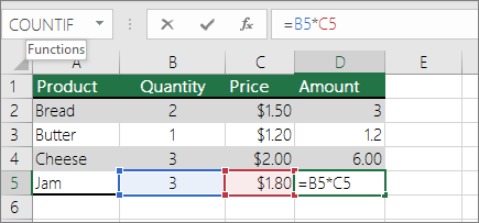
As an example, if you copy the formula =B4*C4 from cell D4 to D5, the formula in D5 adjusts to the right by one column and becomes =B5*C5. If you want to maintain the original cell reference in this example when you copy it, you make the cell reference absolute by preceding the columns (B and C) and row (2) with a dollar sign ($). Then, when you copy the formula =$B$4*$C$4 from D4 to D5, the formula stays exactly the same.
Less often, you may want to mixed absolute and relative cell references by preceding either the column or the row value with a dollar sign—which fixes either the column or the row (for example, $B4 or C$4).
To change the type of cell reference:
-
Select the cell that contains the formula.
-
In the formula bar
 , select the reference that you want to change.
 -
Press F4 to switch between the reference types.
The table below summarizes how a reference type updates if a formula containing the reference is copied two cells down and two cells to the right.
 , select the reference that you want to change.
|
For a formula being copied: |
If the reference is: |
It changes to: |
|
|
$A$1 (absolute column and absolute row) |
$A$1 (the reference is absolute) |
|
A$1 (relative column and absolute row) |
C$1 (the reference is mixed) |
|
|
$A1 (absolute column and relative row) |
$A3 (the reference is mixed) |
|
|
A1 (relative column and relative row) |
C3 (the reference is relative) |
Need more help?
Want more options?
Explore subscription benefits, browse training courses, learn how to secure your device, and more.
Communities help you ask and answer questions, give feedback, and hear from experts with rich knowledge.
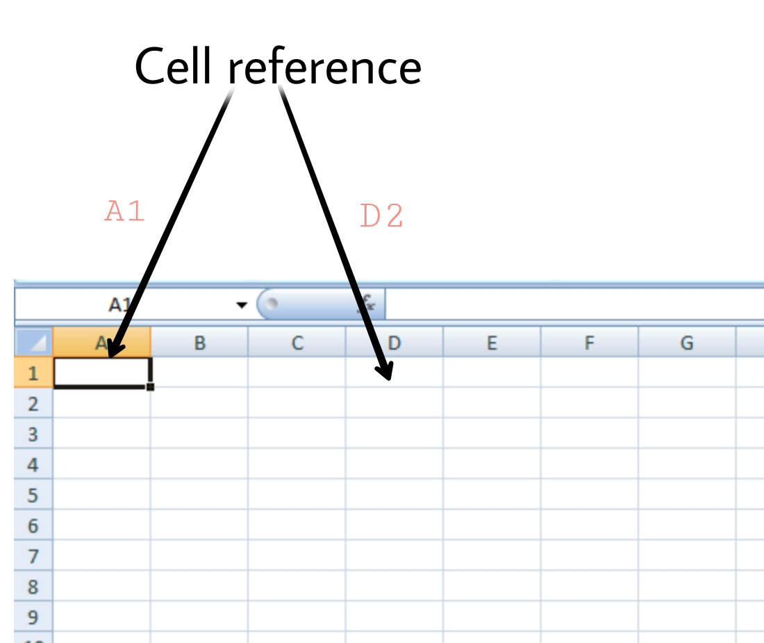
A worksheet in Excel is made up of cells. These cells can be referenced by specifying the row value and the column value.
For example, A1 would refer to the first row (specified as 1) and the first column (specified as A). Similarly, B3 would be the third row and second column.
The power of Excel lies in the fact that you can use these cell references in other cells when creating formulas.
Now there are three kinds of cell references that you can use in Excel:
- Relative Cell References
- Absolute Cell References
- Mixed Cell References
Understanding these different types of cell references will help you work with formulas and save time (especially when copy-pasting formulas).
What are Relative Cell References in Excel?
Let me take a simple example to explain the concept of relative cell references in Excel.
Suppose I have a data set shown below:
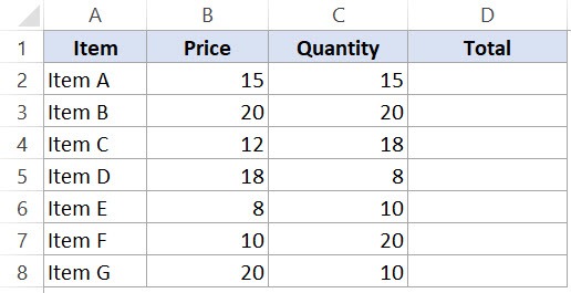
To calculate the total for each item, we need to multiply the price of each item with the quantity of that item.
For the first item, the formula in cell D2 would be B2* C2 (as shown below):
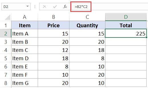
Now, instead of entering the formula for all the cells one by one, you can simply copy cell D2 and paste it into all the other cells (D3:D8). When you do it, you will notice that the cell reference automatically adjusts to refer to the corresponding row. For example, the formula in cell D3 becomes B3*C3 and the formula in D4 becomes B4*C4.
These cell references that adjust itself when the cell is copied are called relative cell references in Excel.
When to Use Relative Cell References in Excel?
Relative cell references are useful when you have to create a formula for a range of cells and the formula needs to refer to a relative cell reference.
In such cases, you can create the formula for one cell and copy-paste it into all cells.
What are Absolute Cell References in Excel?
Unlike relative cell references, absolute cell references don’t change when you copy the formula to other cells.
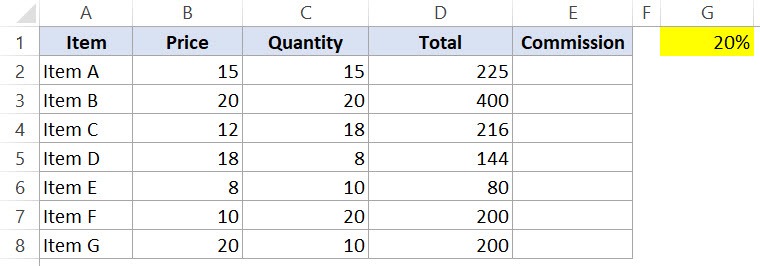
For example, suppose you have the data set as shown below where you have to calculate the commission for each item’s total sales.
The commission is 20% and is listed in cell G1.
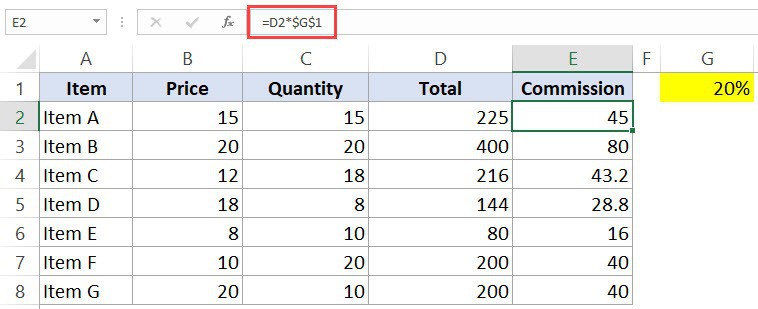
To get the commission amount for each item sale, use the following formula in cell E2 and copy for all cells:
=D2*$G$1
Note that there are two dollar signs ($) in the cell reference that has the commission – $G$2.
What does the Dollar ($) sign do?
A dollar symbol, when added in front of the row and column number, makes it absolute (i.e., stops the row and column number from changing when copied to other cells).
For example, in the above case, when I copy the formula from cell E2 to E3, it changes from =D2*$G$1 to =D3*$G$1.
Note that while D2 changes to D3, $G$1 doesn’t change.
Since we have added a dollar symbol in front of ‘G’ and ‘1’ in G1, it wouldn’t let the cell reference change when it’s copied.
Hence this makes the cell reference absolute.
When to Use Absolute Cell References in Excel?
Absolute cell references are useful when you don’t want the cell reference to change as you copy formulas. This could be the case when you have a fixed value that you need to use in the formula (such as tax rate, commission rate, number of months, etc.)
While you can also hard code this value in the formula (i.e., use 20% instead of $G$2), having it in a cell and then using the cell reference allows you to change it at a future date.
For example, if your commission structure changes and you’re now paying out 25% instead of 20%, you can simply change the value in cell G2, and all the formulas would automatically update.
What are Mixed Cell References in Excel?
Mixed cell references are a bit more tricky than the absolute and relative cell references.
There can be two types of mixed cell references:
- The row is locked while the column changes when the formula is copied.
- The column is locked while the row changes when the formula is copied.
Let’s see how it works using an example.
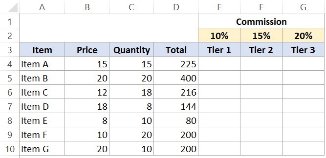
Below is a data set where you need to calculate the three tiers of commission based on the percentage value in cell E2, F2, and G2.
Now you can use the power of mixed reference to calculate all these commissions with just one formula.
Enter the below formula in cell E4 and copy for all cells.
=$B4*$C4*E$2
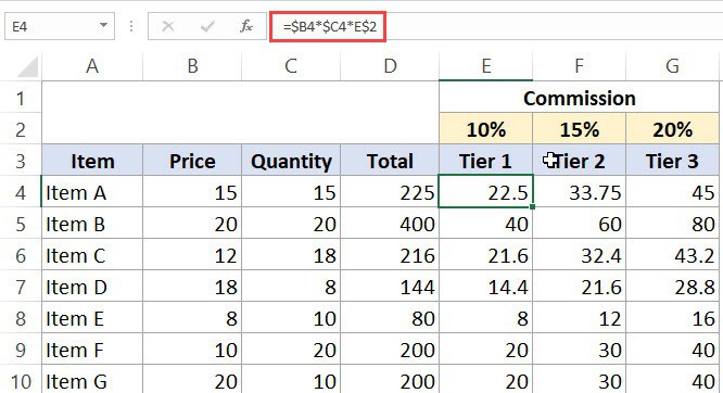
The above formula uses both kinds of mixed cell references (one where the row is locked and one where the column is locked).
Let’s analyze each cell reference and understand how it works:
- $B4 (and $C4) – In this reference, the dollar sign is right before the Column notation but not before the Row number. This means that when you copy the formula to the cells on the right, the reference will remain the same as the column is fixed. For example, if you copy the formula from E4 to F4, this reference would not change. However, when you copy it down, the row number would change as it is not locked.
- E$2 – In this reference, the dollar sign is right before the row number, and the Column notation has no dollar sign. This means that when you copy the formula down the cells, the reference will not change as the row number is locked. However, if you copy the formula to the right, the column alphabet would change as it’s not locked.
How to Change the Reference from Relative to Absolute (or Mixed)?
To change the reference from relative to absolute, you need to add the dollar sign before the column notation and the row number.
For example, A1 is a relative cell reference, and it would become absolute when you make it $A$1.
If you only have a couple of references to change, you may find it easy to change these references manually. So you can go to the formula bar and edit the formula (or select the cell, press F2, and then change it).
However, a faster way to do this is by using the keyboard shortcut – F4.
When you select a cell reference (in the formula bar or in the cell in edit mode) and press F4, it changes the reference.
Suppose you have the reference =A1 in a cell.
Here is what happens when you select the reference and press the F4 key.
- Press F4 key once: The cell reference changes from A1 to $A$1 (becomes ‘absolute’ from ‘relative’).
- Press F4 key two times: The cell reference changes from A1 to A$1 (changes to mixed reference where the row is locked).
- Press F4 key three times: The cell reference changes from A1 to $A1 (changes to mixed reference where the column is locked).
- Press F4 key four times: The cell reference becomes A1 again.
You May Also Like the Following Excel Tutorials:
- How to Copy and Paste Formulas in Excel without Changing Cell References
- How to Lock Cells in Excel.
- Excel Freeze Panes: Use it to Lock Row/Column Headers.
- How to Lock Formulas in Excel.
- How to Reference Another Sheet or Workbook in Excel
- How to Find Circular Reference in Excel
- Using A1 or R1C1 Reference Notation in Excel (& How to Change These)
A absolute reference is excel is a cell reference wherein the column and row coordinates remain fixed on copying a formula from one cell to the other. To fix the coordinates, a dollar sign ($) is placed before them. For example, $D$2 is an absolute reference that refers to cell D2. Shortcut to Absolute Reference in excel is the key F4
The purpose of making the cell reference absolute is to keep it static irrespective of whether the formula is copied to a different worksheet or workbook. By default, a cell reference in Excel is relative (like D2), implying that it changes when the formula is copied.
Apart from absolute and relative, a cell reference can also be mixed. In a mixed reference, either the column label or the row number is kept constant (like $D2 or D$2).
Table of contents
- What is Absolute Reference in Excel?
- Absolute Reference in Excel Shortcut
- How to Use Absolute References in Excel?
- Example #1–Multiplication Formula Using Absolute and Relative References
- Example #2–SUMIFS Formula Using Absolute and Mixed References
- Key Points Related to Cell References of Excel
- Frequently Asked Questions
- Recommended Articles
Absolute Reference in Excel Shortcut
The shortcut to absolute reference in excel is F4. With a single keystroke, the F4 key on your keyboard allows you to add both dollar signs.
How to Use Absolute References in Excel?
While working in Excel, it is essential to know whether a cell reference should stay absolute, relative referenceIn Excel, relative references are a type of cell reference that changes when the same formula is copied to different cells or worksheets. Let’s say we have =B1+C1 in cell A1, and we copy this formula to cell B2 and it becomes C2+D2.read more or mixedA mixed reference is a type of cell reference that differs from absolute and relative cell reference. In the mixed cell reference, we only refer to the column of the cell or the row of the cell.read more. This helps one to carry out the calculations as desired.
With this article, we will focus on absolute references of Excel. Let us consider some examples to understand the working of these references in Excel.
You can download this Absolute Reference Excel Template here – Absolute Reference Excel Template
Example #1–Multiplication Formula Using Absolute and Relative References
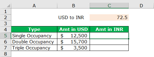
The following image shows the rates (in USD in column B) of different rooms of a hotel. We want to convert each amount from USD to INR (in column C).
Assume that 1 USD is equal to Rs. 72.5. This USD to INR conversion rate is given in cell C2. Use absolute and relative references in the multiplication excel formula. Explain the cell references used for the given task.
The steps to convert the given amounts from USD to INR by using the stated references are listed as follows:
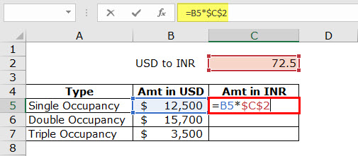
- Begin by typing the “equal to” sign (=) in cell C5. Next, select cell B5 and type the asterisk (*), which is the symbol for multiplication. Then, select cell C2.
Once the reference C2 appears in cell C5, press the F4 key once. This changes the reference from C2 to $C$2. The entire formula (=B5*$C$2) is shown in the following image.

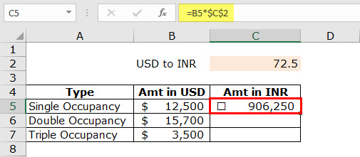
- Once the formula has been entered in cell C5, press the “Enter” key. The output is 906250, as shown in the following image.
Hence, $12,500 is equal to Rs. 906,250. So, the first USD amount has been converted to INR.
Note: Please ignore the small checkbox displayed in cell C5 of the following image.
- Drag the formula of cell C5 till cell C7. For dragging, use the fill handle displayed at the bottom-right corner of cell C5.
The outputs for the range C5:C7 are shown in the following image. Notice that though cells C5, C6, and C7 are selected, the formula of only cell C5 is shown in the formula bar. Further, the output of cell C7 is shown in a red box.
Note: Please ignore the checkboxes appearing in cells C5, C6, and C7 on the left side. These checkboxes are not an outcome of the multiplication formula entered in these cells.

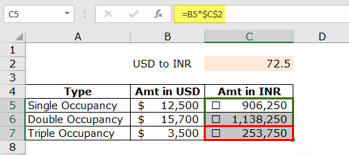
Explanation of the cell references: In the formulas of column C, the first cell reference is relative (B5, B6, and B7), while the second cell reference is absolute ($C$2). The reason is that on copying the formula from cell C5 to C7, we wanted the first reference to change and the second reference to stay constant.
As a result, B5 (in cell C5) changes to B6 (in cell C6) and further changes to B7 (in cell B7). However, the reference $C$2 stays the same in cells C5, C6, and C7. So, the aim is to multiply the different amounts of column B with the same conversion rate of cell C2.
Example #2–SUMIFS Formula Using Absolute and Mixed References
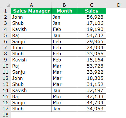
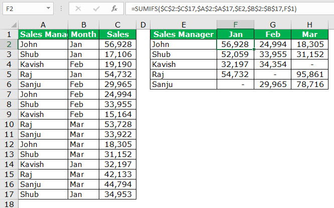
The following image shows the sales revenue generated (in $ in column C) in three months (column B) by five sales managers (in column A) of an organization. The three months are January, February, and March. The five sales managers are John, Shub, Kavish, Raj, and Sanju.
Since some sales managers have made multiple sales in a month, their names appear more than once against a single month. Sum the sales revenues generated by each manager in a particular month. Use the SUMIFS function of Excel.
Further, use the following types of cell references for the given task:
- For “sum_range,” “criteria_range1,” and “criteria_range2,” use absolute excel references.
- For “criteria1” and “criteria2,” use mixed references.
Explain the formula and the cell references used.
The steps to perform the given task by using the SUMIFS functionSUMIFS is an enhanced version of the SUMIF formula in Excel that enables you to sum any range of data by matching several criteria. read more and the stated references are listed as follows:
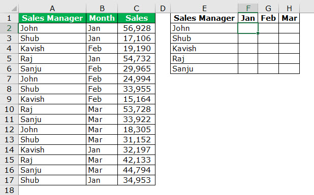
Step 1: Write the names of the five managers in the range E2:E6. Enter the names of the three months in the range F1 to H1. All these names (shown in the following image) will be used in the SUMIFS formula one at a time.
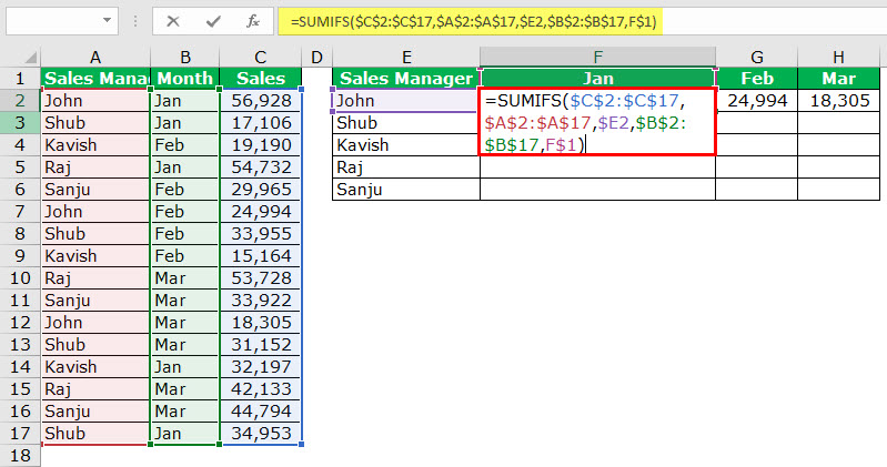
Step 2: Enter the following formula in cell F2.
“=SUMIFS($C$2:$C$17,$A$2:$A$17,$E2,$B$2:$B$17,F$1)”
This is shown in the succeeding image.
Note: Please ignore the figures of cells G2 and H2 at this step.
Step 3: Drag the formula of cell F2 horizontally (till cell H2) and vertically (till cell F6). Likewise, drag the formula of cells F3, F4, F5, and F6 horizontally till cells H3, H4, H5, and H6 respectively.
The outputs of all the SUMIFS formulas are shown in the range F2:H6 of the following image. Hence, the sales revenue generated by all the managers in the given months (January, February, and March) has been obtained.
Notice that the cells containing a hyphen (F6, G5, and H4) imply that a sale has not been made in that month by the respective manager.
Explanation of the formula and the cell references: The formula of step 1 works as follows:
- The “sum_range” supplied to the SUMIFS function is $C$2:$C$17. The numbers of this range are summed subject to the conditions (or criteria) entered in the formula. We have used absolute cell references in the “sum_range.” This is because we do not want the references to change as the formula is copied to the remaining cells of the range F2:H6.
- The “criteria_range1” supplied to the SUMIFS function is $A$2:$A$17. This range is evaluated for “criteria1.” We have again used absolute excel references in “criteria_range1.” The reason is that the “criteria_range1” stays the same across all the SUMIFS formulas of the range F2:H6.
- The “criteria1” supplied to the SUMIFS function is $E2. Since cell E2 contains the name “John,” the SUMIFS function checks the range A2:A17 for this name. We have used a mixed reference ($E2) for “criteria1” because we want its column label (E) to be fixed and the row number (2) to be variable. This enables the SUMIFS function to check the range A2:A17 for the values of cells E2, E3, E4, E5, and E6. So, each cell of column E (rows 2 to 6) serves as “criteria 1” in the different SUMIFS formulas of the range F2:H6.
- The “criteria_range2” supplied to the SUMIFS function is $B$2:$B$17. This range is evaluated for “criteria2.” We have used absolute references in this range because we want the same range (B2:B17) to be evaluated each time for “criteria2.”
- The “criteria2” supplied to the SUMIFS function is F$1. Cell F1 contains the value “Jan.” So, the SUMIFS function checks the range B2:B17 for the value “Jan.” We have used a mixed reference (F$1) for “criteria2.” This is because we want the SUMIFS function to check the range B2:B17 for the values of cells F1, G1, and H1. Thus, the column label changes from F to G and finally to H, while the row number stays constant at 1.
The SUMIFS formula of step 1 checks for two conditions (criteria) “John” and “Jan” in the ranges A2:A17 and B2:B17 respectively. Further, those values of the range C2:C17 are summed that satisfy both these conditions. So, only the number 56,928 satisfies both these conditions. Hence, the output is 56,928.
In the same way, the SUMIFS formulas of the remaining range F2:H6 work.
Note: The SUMIFS function sums those values that satisfy multiple criteria. For the syntax of the SUMIFS function, click the hyperlink given before step 1 of this example.
The important points related to cell references of Excel are listed as follows:
- In an absolute reference in excel, both the column label and the row number are fixed by placing a dollar sign ($) before them. So, an absolute reference has an absolute column and an absolute row.
- In a relative reference, both the column label and the row number are variable. The dollar sign ($) is omitted in a relative reference. So, a relative reference has a relative column and a relative row.
- In a mixed reference, either the column label or the row number is fixed, while the other is variable. The dollar sign ($) is placed before the constant part of a mixed reference. So, a mixed reference has either a relative column and an absolute row or an absolute column and a relative row.
- The absolute references in excel do not change irrespective of an upward, downward, leftward or rightward movement of the formula containing them.
- The cell references change each time the F4 key is pressed. They change as follows:
- Pressing the F4 key once changes the cell reference from relative to absolute (like D2 changes to $D$2).
- Pressing the F4 key twice changes the cell reference from absolute to mixed (like $D$2 changes to D$2). The column label of the mixed reference becomes variable, while the row number stays fixed.
- Pressing the F4 key thrice changes the cell reference from mixed to mixed again (like D$2 changes to $D2). The column label of the mixed reference becomes fixed, while the row number stays variable.
- Pressing the F4 key four times changes the cell reference from mixed to relative again (like $D2 changes to D2).
Note: The steps to change a cell reference within a formula are listed as follows:
- Double-click the cell containing the formula.
- Select the cell reference to be changed.
- Press the F4 key the required number of times.
- Complete the formula in the usual way once the cell reference has been changed. So, press either the “Enter” or the “Ctrl+Shift+Enter” keys depending on whether it is a regular or an array formula.
To exit the Edit mode without changing the formula, press the escape (Esc) key.
Frequently Asked Questions
1. Define an absolute cell reference and suggest how to create it in Excel.
An absolute reference in excel is one in which both the column label and the row number are fixed by placing a dollar sign ($) before them. For example, $H$5 is an absolute cell reference.
To create an absolute cell reference in Excel, follow either of the listed methods:
• Insert a dollar sign ($) in the cell reference manually. This sign should precede the column label and the row number.
• Enter a relative reference and press the F4 key to make it absolute. This key should be pressed only once.
Note: To insert a relative reference in a formula, simply select the cell or the range to be referenced. Excel inserts a relative reference by default.
2. When should absolute references be used in Excel? State how to remove them from a cell of Excel.
Absolute references of Excel should be used in the following situations:
a. When there is a need to move the formula to a different worksheet or workbook without impacting the cell references
b. When the formula needs to be dragged to the remaining cells of the range, but the column and row coordinates should stay fixed
c. When multiple calculations need to be performed by referring to a particular cell again and again
Removing absolute references from a cell implies changing them to either mixed or relative references. For this, follow either of the listed methods:
• Manually delete the dollar sign ($), which precedes the column label and/or the row number. The cell reference changes to either mixed or relative depending on the number of deletions made.
• Double-click the cell containing the formula. Select the absolute cell reference and press the F4 key once. The cell reference changes to mixed where the column label is variable and the row number is fixed.
Note: Once the reference has been changed in the preceding bullet points, press either the “Enter” or the “Ctrl+Shift+Enter” keys to complete the formula.
3. Differentiate between absolute and relative cell references of Excel.
The differences between absolute and relative cell references are listed as follows:
a. Absolute references stay static irrespective of where they are copied, while relative references change when copied to a different location.
b. In an absolute reference, both column and row coordinates are fixed. On the other hand, in a relative reference, both column and row coordinates are variable.
c. An absolute reference is used when calculations involve a specific cell to be referred multiple times. In contrast, a relative reference is used when the same calculation needs to be repeated across various columns and/or rows.
d. An absolute reference is inserted either manually or by pressing the F4 key. In comparison, a relative reference is inserted by simply selecting the cell or the range to be referenced.
Before applying formulas in Excel, it is essential to know the differences between the two cell references (absolute and relative). This helps choose the appropriate cell reference.
Recommended Articles
This has been a guide to Absolute Reference in Excel. Here we explain how to use Absolute Cell Reference in Excel along its shortcut and practical examples. You may also look at these useful tools of Excel–
- Relative References in ExcelIn Excel, relative references are a type of cell reference that changes when the same formula is copied to different cells or worksheets. Let’s say we have =B1+C1 in cell A1, and we copy this formula to cell B2 and it becomes C2+D2.read more
- Watch Window in Excel
- Formatting in Excel
- How to Name Range in Excel?Name range in Excel is a name given to a range for the future reference. To name a range, first select the range of data and then insert a table to the range, then put a name to the range from the name box on the left-hand side of the window.read more
Cell reference is the address or name of a cell or a range of cells. It is the combination of column name and row number. It helps the software to identify the cell from where the data/value is to be used in the formula. We can reference the cell of other worksheets and also of other programs.
- Referencing the cell of other worksheets is known as External referencing.
- Referencing the cell of other programs is known as Remote referencing.
There are two types of cell references in Excel:
- Relative reference
- Absolute reference
Relative Reference
Relative reference is the default cell reference in Excel. It is simply the combination of column name and row number without any dollar ($) sign. When you copy the formula from one cell to another the relative cell address changes depending on the relative position of column and row. C1, D2, E4, etc are examples of relative cell references. Relative references are used when we want to perform a similar operation on multiple cells and the formula must change according to the relative address of column and row.
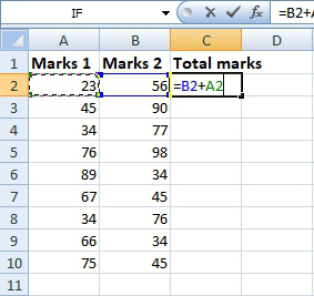
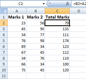
For example, We want to add the marks of two subjects entered in column A and column B and display the result in column C. Here, we will use relative reference so that the same rows of column’s A and B are added.
Steps to Use Relative Reference:
Step 1: We write the formula in any cell and press enter so that it is calculated. In this example, we write the formula(= B2 + A2) in cell C2 and press enter to calculate the formula.
Step 2: Now click on the Fill handle at the corner of cell which contains the formula(C2).

Step 3: Drag the Fill handle up to the cells you want to fill. In our example, we will drag it till cell C10.
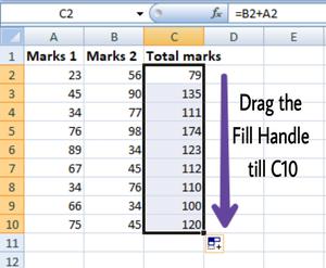
Step 4: Now we can see that the addition operation is performed between the cell A2 and B2, A3 and B3 and so on.
Step 5: You can double-click on any cell to check that the operation is performed in between which cells.
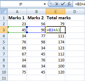
Thus, in the above example, we see that the relative address of cell A2 changes to A3, A4, and so on, similarly the relative address changes for column B, depending on the relative position of the row.
Absolute Reference
Absolute reference is the cell reference in which the row and column are made constant by adding the dollar ($) sign before the column name and row number. The absolute reference does not change as you copy the formula from one cell to other. If either the row or the column is made constant then it is known as a mixed reference. You can also press the F4 key to make any cell reference constant. $A$1, $B$3 are examples of absolute cell reference.
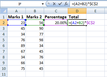
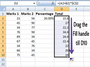
For example, We want to multiply the sum of marks of two subjects, entered in column A and column B, with the percentage entered in cell C2 and display the result in column D. Here, we will use absolute reference so that the address of cell C2 remains constant and does not change with the relative position of column and rows.
Steps to Use Absolute Reference:
Step 1: We write the formula in any cell and press enter so that it is calculated. In this example, we write the formula(=(A2+B2)*$C$2) in cell D2 and press enter to calculate the formula.
Step 2: Now click on the Fill handle at the corner of cell which contains the formula(D2).
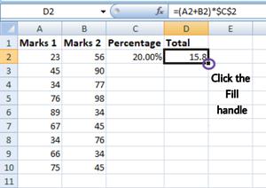
Step 3: Drag the Fill handle up to the cells you want to fill. In our example, we will drag it till cell D10.
Step 4: Now we can see that the percentage is calculated in column D.
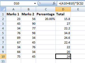
Step 5: You can double-click on any cell to check that the operation is performed in between which cells, and we see that the address of cell C2 does not change.
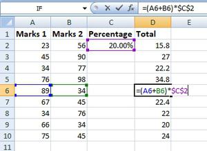
Thus, in the above example we see that the address of cell C2 is not changed whereas the address of column A and B changes with the relative position of the row and column, this happened because we used the absolute address of the cell C2.
Absolute Reference in Excel (Table of Contents)
- Absolute Cell Reference in Excel
- How to Create Absolute Cell Reference in Excel?
- How to Use Absolute Cell Reference in Excel?
Introduction to Absolute Cell Reference in Excel
Absolute reference in excel is used when we want to fix the position of the selected cell in any formula so that its value will be not changed whenever we are changing the cell or copying the formula to other cells or sheets. This is done by putting the dollar (“$”) sign before and after the column name of the selected cell. Or else, we can type the F4 function key, which will automatically cover the column alphabet with the dollar. For example, if you want to fix cell A1, then it will look as “=$A$1”.
Uses of Absolute Cell Reference in Excel
The absolute cell reference in excel is a cell address that contains a dollar sign ($). It can precede the column reference, the row reference or both. With an absolute cell reference in excel, we can keep a row or a column constant or keep both constant. It doesn’t change when copied to other cells.
How to Create an Absolute Cell Reference in Excel?
Below are the steps to convert a cell address into an absolute cell reference:
- Select a cell where you want to create an absolute cell reference. Suppose cell A1.
- =A1 – It is a relative reference by default. However, to create an absolute reference, we need to add a dollar sign ($) before the column or row coordinates.
- =$A1 – If we put a $ dollar sign before the column coordinate (A), it will only lock the column. This means that when we copy or drag this formula cell to other cells in the same row, the column will remain fixed at A, while the row coordinate will change.
- =A$1 – If we put a $ dollar sign before the row coordinate (1), it will lock only rows. This means that when we copy or drag this cell to other cells in the same column, the row coordinate will remain fixed at 1, while the column coordinate will change.
- =$A$1 – It’s called an absolute cell reference, and it locks both the row and the column. It means that if we drag or copy this cell, the formula cell will remain constant, i.e., it will always refer to cell A1, no matter where it is copied or dragged.
How to Use Absolute Cell Reference in Excel?
Let’s take some examples to understand the use of an absolute cell reference in excel.
You can download this Absolute Reference Excel Template here – Absolute Reference Excel Template
Absolute Reference in Excel – Example #1
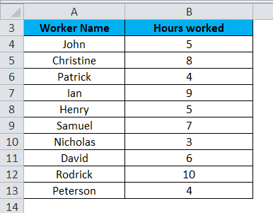
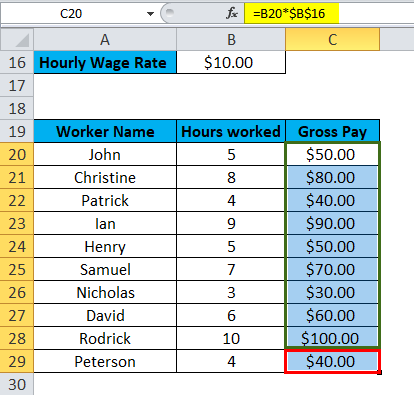
In the below table, data is available for a group of workers, including their names and the corresponding number of hours worked. The hourly wage rate is $10.00 per hour. We need to calculate the gross pay for each worker based on their hours worked.
Solution:
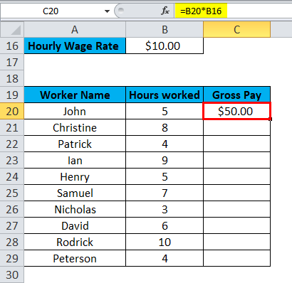
We will input the hourly wage rate amount of $10 in cell B16. Then, as seen in the image below, to calculate the gross pay for the first employee (John), we will multiply the fixed-wage hourly rate of $10.00 (cell B16) by the number of hours worked (cell B20). Therefore, we will enter the formula “=B20*B16” in cell C20.

The result is $50, as shown below.
However, if we drag the formula and paste it into the corresponding cells in each row for the other workers, it will give incorrect results, as shown in the below image. This is because the fixed-wage hourly rate is changing for each worker.

To fix this, we must make the cell containing the fixed-wage hourly rate an absolute cell reference by adding a $ sign before the column name and row number.
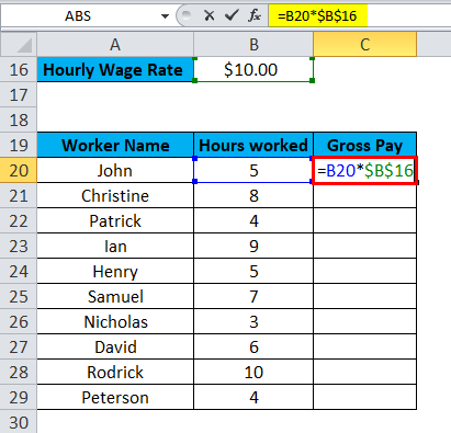
We can put a $ dollar sign before the column name and before the row number, like this – $B$16. The result is shown below.
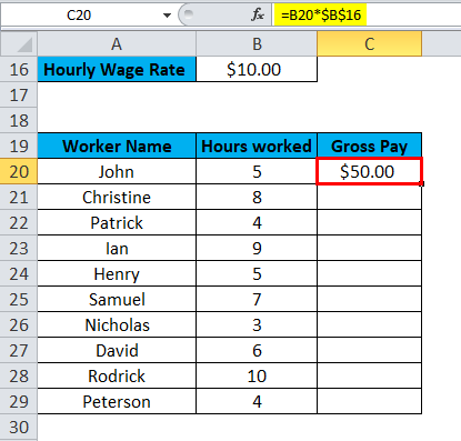
Through this, we can lock the value of B16 for all workers. Now, we can drag this formula for the rest of the workers to recalculate their gross pay.
Note: You can use the F4 key as a shortcut to make a cell an absolute cell reference. It automatically inserts a dollar sign in both places.
Absolute Reference in Excel – Example #2
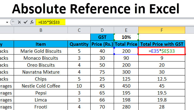
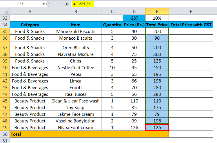
Alice went to a retail shop and purchased about 15 groceries and beauty products. Each item has a GST rate of 10%. To calculate the Net Amount, we need to determine the tax rate for each item.
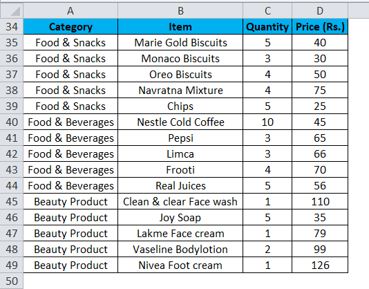
Solution:
First, we will calculate the total price of each item by multiplying the no. of items by the corresponding product price.
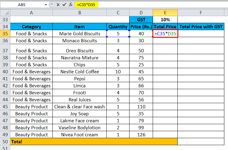
The result is seen below.
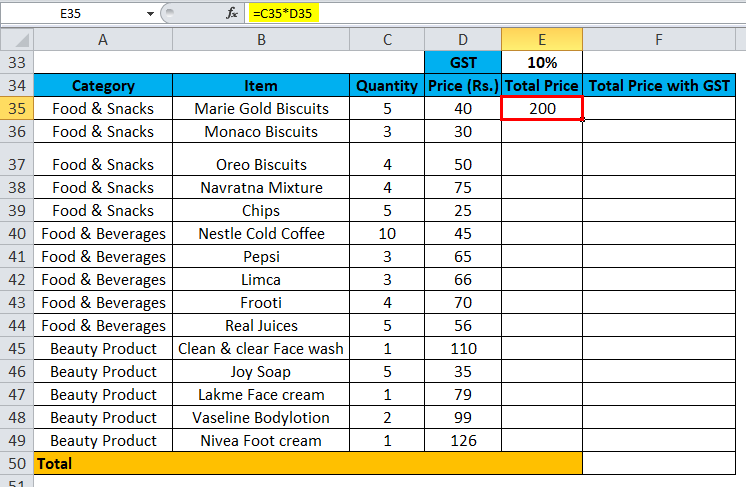
Drag this formula for the rest of the products to get their total prices.
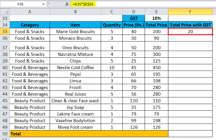
To calculate the tax rate for each product, multiply the total price by the GST rate (which is 10%).
Use an absolute cell reference for the GST rate by making cell E33 an absolute reference using the F4 key. This will add a $ sign before E and 33 like this – $E$33
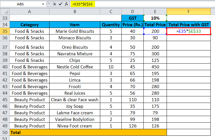
The result is 20.
Drag this formula for the rest of the products to get their tax rates. For instance, the formula in cell F49 is =E35*$E$33.
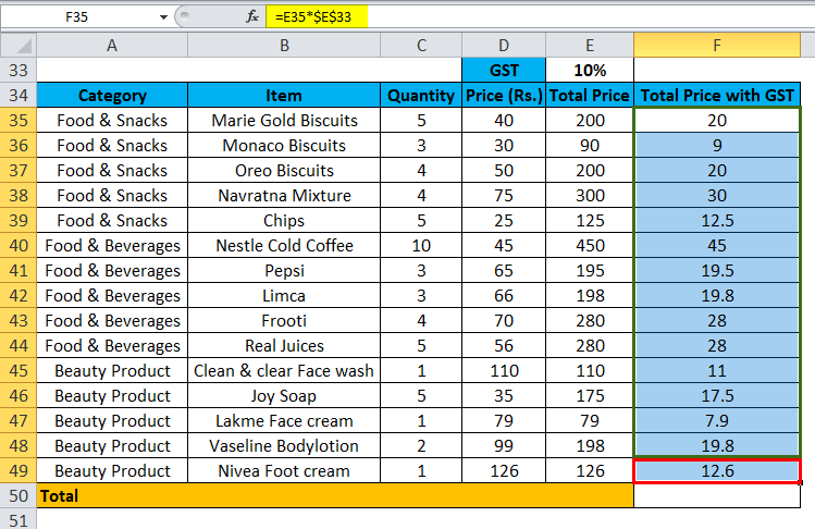
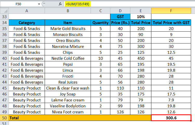
To calculate the net amount, add the total price with the GST for each product using the SUM Function in excel.
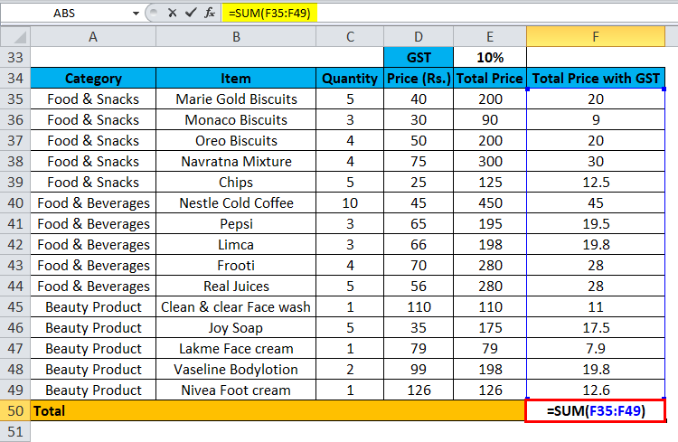
The final result is Rs. 300.60 (the sum of the net amounts for all the products).
Advanced Techniques
There are several advanced techniques you can use with absolute references in Excel. Here are a few examples:
#1 Using Absolute References to Create Dynamic Range Names
You can use absolute references to create dynamic range names that automatically adjust depending on the data size.
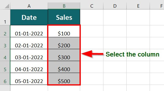
Suppose you have a dataset as shown below. To create a dynamic range name for the Sales column, follow these steps:
|
Date |
Sales |
| 01/01/2022 | $100 |
| 02/01/2022 | $200 |
| 03/01/2022 | $300 |
| 04/01/2022 | $400 |
| 05/01/2022 | $500 |
1. Select the entire column (in this case, B2:B6).
2. Click on the “Formulas” tab, and then click on “Define Name” in the “Defined Names” section.
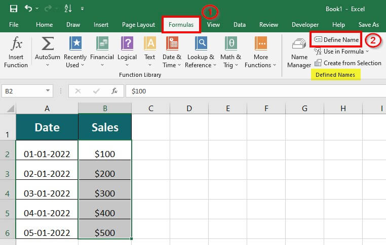
3. In the “New Name” dialog box, enter a name for the range (e.g., “SalesData“).
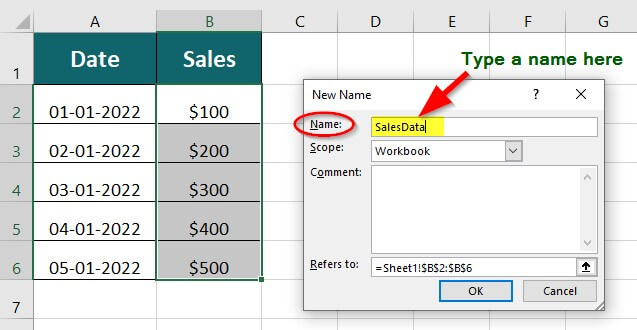
4. In the “Refers to” field, enter the formula =OFFSET(Sheet1!$B$2,0,0,COUNTA(Sheet1!$B:$B)-1,1), and then click OK.
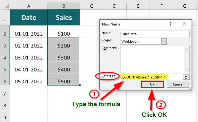
This will create a dynamic range name that adjusts automatically when new data gets added to the Sales column.
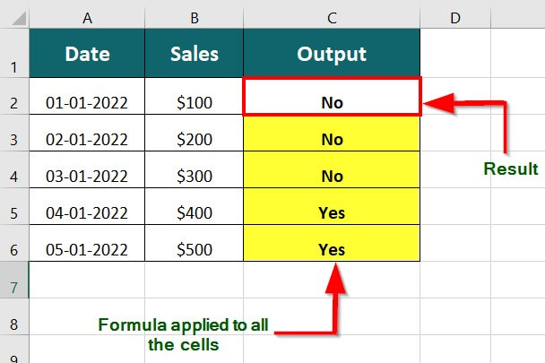
#2 Using Absolute References with IF Function
You can use absolute references with the IF function to perform calculations based on specific criteria.
Suppose you have the following dataset:
|
Date |
Sales |
| 01/01/2022 | $100 |
| 02/01/2022 | $200 |
| 03/01/2022 | $300 |
| 04/01/2022 | $400 |
| 05/01/2022 | $500 |
To use Absolute References with the IF function, follow these steps:
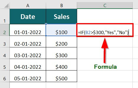
1. In cell C2, enter the formula =IF(B2>$300,”Yes”,”No”).
2. Copy the formula down to the rest of the cells in column C.
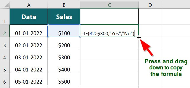
This will use an absolute reference to compare each value in the Sales column to a fixed value ($300 in this case) and return “Yes” if the value exceeds $300.
Things to Remember
- Use relative references when appropriate: Relative references can make your formulas simpler and easier to read, especially for simple calculations. Reserve absolute references for situations where you must lock a specific cell or range of cells.
- Understand the difference between references: Excel also allows for mixed references, enabling you to lock only one part of a cell reference while leaving the other relative. Ensure you understand the difference and choose the appropriate reference type for your needs.
- Avoid circular references: A circular reference is when a formula returns to its cell, forming an endless loop. This can cause errors in a spreadsheet.
- Document your formulas: If you share your spreadsheet with others or need to refer to it later, document them. So that others can understand how they work and troubleshoot any issues.
- Use named ranges: Rather than referencing cells in your formulas, consider using named ranges to make your formulas easier to understand and sustain.
- Use comments: If your formulas are particularly complex, consider using comments to explain how they work and why you chose to use absolute references in certain places.
- Separate sheet for formulas: If you have many complex formulas in your spreadsheet, consider creating a separate sheet for storing and documenting your formulas. This can make managing and troubleshooting your formulas easier, especially if you need to make changes later.
Common Errors
There are a few common errors that people make when using absolute references in Excel. Some of these errors include:
- Forgetting to use the dollar sign: When creating an absolute reference, it is essential to utilize the sign of dollar ($) before the column and row of the cell reference to lock it. If you forget to do this, Excel will interpret it as a relative reference, which can result in incorrect calculations.
- Using the wrong reference: It’s easy to reference the wrong cell when using absolute references, especially when working with large datasets. This can happen if you accidentally select the wrong cell or change the position of the referenced cell without updating the formula.
- Copying and pasting incorrectly: When copying and pasting formulas that contain absolute references, you need to make sure that you select the correct cell when pasting the formula. If you paste the formula into the wrong cell, the absolute reference may not point to the intended cell, resulting in incorrect calculations.
- Forgetting to lock the correct cell: When creating an absolute reference, it’s important to lock it using the dollar sign. If you lock the wrong cell or forget to lock it, it can lead to errors in your calculations.
- Using absolute references unnecessarily: While they can be helpful in certain situations, they can make your formulas more complex and harder to read. It’s important to use them judiciously and only when necessary.
- Failing to update absolute references: If you change the location of cells or ranges referenced in your absolute reference, you must update the reference accordingly. Forgetting to do so can guide you to errors in your calculations.
Advantages of Absolute References
- Saves Time: Using absolute references in Excel saves you time when copying formulas across many cells. The fixed value or formula can be in reference without manually updating each cell. This is particularly useful when working with large data sets or complex formulas.
- Accuracy: Absolute references can help ensure the accuracy of formulas by keeping specific values constant. This is especially useful when working with complex formulas that reference many cells. By using absolute references, you can be confident that the formula will always produce the correct result, regardless of changes to other cells.
- Customization: Absolute references are customizable in Excel, allowing you to choose which cells to remain fixed and which cells you want to be relative. This flexibility creates formulas that adapt to different situations, like changes in input variables or data structure.
- Replication: Absolute references help replicate formulas with fixed values, such as commission calculations. By creating an absolute reference to the fixed value, you can copy the formula to other cells without manually adjusting each one. This can save time and reduce the risk of errors.
- Improved readability: Absolute references make formulas easier to read and understand. They show which cells contain constants and variables. By fixing specific values in your formulas, you can show which cells are input and output, making the formula easier to follow.
- Consistent formatting: Absolute references ensure that your Excel sheets are consistent. You can keep your formulas and charts neat and tidy by fixing certain cells and ranges, even adding or removing data. This can make reading and understanding the data easier and help prevent formatting errors.
Disadvantages of Absolute References
- Harder to Read: While absolute references can offer benefits, they can make formulas more complex and harder to read. This is particularly true when you have many absolute references in the same formula. In this case, the formula can become difficult to understand and troubleshoot, especially if you didn’t create it yourself.
- Error-Prone: Absolute references can be error-prone if you forget to lock the correct cells. This can lead to incorrect calculations and wasting time troubleshooting the issue. Suppose you forget to lock the cell that contains the fixed tax rate in a sales tax calculation formula. Here, copying the formula to other cells may result in incorrect calculations.
- Potential for Data Inaccuracy: While absolute references can help ensure accuracy by keeping specific values constant, they can also lead to data inaccuracy if the referenced cell or range of cells contains incorrect data. For example, suppose the cell containing the fixed tax rate in a sales tax calculation formula has the wrong value. In that case, all the cells referencing that cell will also produce incorrect results.
- Difficulty Adapting to Changes: Using absolute references can make it more difficult to adapt to changes in data, especially if you need to change the cells that contain fixed values. In this case, you may need to update all the formulas referencing the fixed cells, which can be time-consuming and prone to errors.
- Limits Flexibility: While absolute references can allow you to choose which cells to fix and which to be relative to, they can also limit flexibility by fixing cells you may want to change. For example, if you create a formula that references a cell containing a date, using an absolute reference will fix the date to the specific cell, making it difficult to change the date without changing the formula.
Relative vs Absolute References
|
Aspect |
Relative References |
Absolute References |
| Definition | References that adjust with cell movement | References that remain constant despite movement |
| Denoted By | Denoted by cell references without dollar signs | It was Denoted by cell references with dollar signs |
| Change | Change based on where they are copied or moved | Remain fixed regardless of where they are copied or moved |
| Usage | Useful when creating formulas that need to be adjusted based on location | Useful when creating formulas that need to reference specific cells |
| Syntax | A referenced cell gets indicated by its position | A referenced cell gets indicated by its cell address |
| Example | If you copy a formula that refers to cell A1 and pastes it into cell B1, the reference in the formula will change from A1 to B1. | If you copy a formula that refers to cell A1 and pastes it into cell B1, the reference will remain A1. |
Recommended Articles
This has been a guide to Absolute Reference in Excel. Here we discuss its uses and how to create Absolute Cell References along with excel examples and downloadable excel templates. You may also look at these useful tools in excel –
- 3D Cell Reference in Excel
- Mixed Reference in Excel
- Excel Circular Reference
- Interesting Excel reference percentage absolute and relative