
What’s in the name?
If you are working with Excel spreadsheets, it could mean a lot of time saving and efficiency.
In this tutorial, you’ll learn how to create Named Ranges in Excel and how to use it to save time.
Named Ranges in Excel – An Introduction
If someone has to call me or refer to me, they will use my name (instead of saying a male is staying in so and so place with so and so height and weight).
Right?
Similarly, in Excel, you can give a name to a cell or a range of cells.
Now, instead of using the cell reference (such as A1 or A1:A10), you can simply use the name that you assigned to it.
For example, suppose you have a data set as shown below:
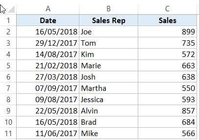
In this data set, if you have to refer to the range that has the Date, you will have to use A2:A11 in formulas. Similarly, for Sales Rep and Sales, you will have to use B2:B11 and C2:C11.
While it’s alright when you only have a couple of data points, but in case you huge complex data sets, using cell references to refer to data could be time-consuming.
Excel Named Ranges makes it easy to refer to data sets in Excel.
You can create a named range in Excel for each data category, and then use that name instead of the cell references. For example, dates can be named ‘Date’, Sales Rep data can be named ‘SalesRep’ and sales data can be named ‘Sales’.

You can also create a name for a single cell. For example, if you have the sales commission percentage in a cell, you can name that cell as ‘Commission’.
Benefits of Creating Named Ranges in Excel
Here are the benefits of using named ranges in Excel.
Use Names instead of Cell References
When you create Named Ranges in Excel, you can use these names instead of the cell references.
For example, you can use =SUM(SALES) instead of =SUM(C2:C11) for the above data set.
Have a look at ṭhe formulas listed below. Instead of using cell references, I have used the Named Ranges.
- Number of sales with value more than 500: =COUNTIF(Sales,”>500″)
- Sum of all the sales done by Tom: =SUMIF(SalesRep,”Tom”,Sales)
- Commission earned by Joe (sales by Joe multiplied by commission percentage):
=SUMIF(SalesRep,”Joe”,Sales)*Commission
You would agree that these formulas are easy to create and easy to understand (especially when you share it with someone else or revisit it yourself.
No Need to Go Back to the Dataset to Select Cells
Another significant benefit of using Named Ranges in Excel is that you don’t need to go back and select the cell ranges.
You can just type a couple of alphabets of that named range and Excel will show the matching named ranges (as shown below):

Named Ranges Make Formulas Dynamic
By using Named Ranges in Excel, you can make Excel formulas dynamic.
For example, in the case of sales commission, instead of using the value 2.5%, you can use the Named Range.
Now, if your company later decides to increase the commission to 3%, you can simply update the Named Range, and all the calculation would automatically update to reflect the new commission.
How to Create Named Ranges in Excel
Here are three ways to create Named Ranges in Excel:
Method #1 – Using Define Name
Here are the steps to create Named Ranges in Excel using Define Name:
This will create a Named Range SALESREP.
Method #2: Using the Name Box
- Select the range for which you want to create a name (do not select headers).
- Go to the Name Box on the left of Formula bar and Type the name of the with which you want to create the Named Range.

- Note that the Name created here will be available for the entire Workbook. If you wish to restrict it to a worksheet, use Method 1.
Method #3: Using Create From Selection Option
This is the recommended way when you have data in tabular form, and you want to create named range for each column/row.
For example, in the dataset below, if you want to quickly create three named ranges (Date, Sales_Rep, and Sales), then you can use the method shown below.
Here are the steps to quickly create named ranges from a dataset:
This will create three Named Ranges – Date, Sales_Rep, and Sales.
Note that it automatically picks up names from the headers. If there are any space between words, it inserts an underscore (as you can’t have spaces in named ranges).
Naming Convention for Named Ranges in Excel
There are certain naming rules you need to know while creating Named Ranges in Excel:
- The first character of a Named Range should be a letter and underscore character(_), or a backslash(). If it’s anything else, it will show an error. The remaining characters can be letters, numbers, special characters, period, or underscore.
- You can not use names that also represent cell references in Excel. For example, you can’t use AB1 as it is also a cell reference.
- You can’t use spaces while creating named ranges. For example, you can’t have Sales Rep as a named range. If you want to combine two words and create a Named Range, use an underscore, period or uppercase characters to create it. For example, you can have Sales_Rep, SalesRep, or SalesRep.
- While creating named ranges, Excel treats uppercase and lowercase the same way. For example, if you create a named range SALES, then you will not be able to create another named range such as ‘sales’ or ‘Sales’.
- A Named Range can be up to 255 characters long.
Too Many Named Ranges in Excel? Don’t Worry
Sometimes in large data sets and complex models, you may end up creating a lot of Named Ranges in Excel.
What if you don’t remember the name of the Named Range you created?
Don’t worry – here are some useful tips.
Getting the Names of All the Named Ranges
Here are the steps to get a list of all the named ranges you created:
This will give you a list of all the Named Ranges in that workbook. To use a named range (in formulas or a cell), double click on it.

Displaying the Matching Named Ranges
- If you have some idea about the Name, type a few initial characters, and Excel will show a drop down of the matching names.


How to Edit Named Ranges in Excel
If you have already created a Named Range, you can edit it using the following steps:
Useful Named Range Shortcuts (the Power of F3)
Here are some useful keyboard shortcuts that will come handy when you are working with Named Ranges in Excel:
- To get a list of all the Named Ranges and pasting it in Formula: F3
- To create new name using Name Manager Dialogue Box: Control + F3
- To create Named Ranges from Selection: Control + Shift + F3
Creating Dynamic Named Ranges in Excel
So far in this tutorial, we have created static Named Ranges.
This means that these Named Ranges would always refer to the same dataset.
For example, if A1:A10 has been named as ‘Sales’, it would always refer to A1:A10.
If you add more sales data, then you would have to manually go and update the reference in the named range.
In the world of ever-expanding data sets, this may end up taking up a lot of your time. Every time you get new data, you may have to update the Named Ranges in Excel.
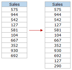
To tackle this issue, we can create Dynamic Named Ranges in Excel that would automatically account for additional data and include it in the existing Named Range.
For example, For example, if I add two additional sales data points, a dynamic named range would automatically refer to A1:A12.
This kind of Dynamic Named Range can be created by using Excel INDEX function. Instead of specifying the cell references while creating the Named Range, we specify the formula. The formula automatically updated when the data is added or deleted.
Let’s see how to create Dynamic Named Ranges in Excel.
Suppose we have the sales data in cell A2:A11.

Here are the steps to create Dynamic Named Ranges in Excel:
-
- Go to the Formula tab and click on Define Name.

- In the New Name dialogue box type the following:
- Name: Sales
- Scope: Workbook
- Refers to: =$A$2:INDEX($A$2:$A$100,COUNTIF($A$2:$A$100,”<>”&””))

- Click OK.
- Go to the Formula tab and click on Define Name.


Done!
You now have a dynamic named range with the name ‘Sales’. This would automatically update whenever you add data to it or remove data from it.
How does Dynamic Named Ranges Work?
To explain how this work, you need to know a bit more about Excel INDEX function.
Most people use INDEX to return a value from a list based on the row and column number.
But the INDEX function also has another side to it.
It can be used to return a cell reference when it is used as a part of a cell reference.
For example, here is the formula that we have used to create a dynamic named range:
=$A$2:INDEX($A$2:$A$100,COUNTIF($A$2:$A$100,"<>"&""))
INDEX($A$2:$A$100,COUNTIF($A$2:$A$100,”<>”&””) –> This part of the formula is expected to return a value (which would be the 10th value from the list, considering there are ten items).
However, when used in front of a reference (=$A$2:INDEX($A$2:$A$100,COUNTIF($A$2:$A$100,”<>”&””))) it returns the reference to the cell instead of the value.
Hence, here it returns =$A$2:$A$11
If we add two additional values to the sales column, it would then return =$A$2:$A$13
When you add new data to the list, Excel COUNTIF function returns the number of non-blank cells in the data. This number is used by the INDEX function to fetch the cell reference of the last item in the list.
Note:
- This would only work if there are no blank cells in the data.
- In the example taken above, I have assigned a large number of cells (A2:A100) for the Named Range formula. You can adjust this based on your data set.
You can also use OFFSET function to create a Dynamic Named Ranges in Excel, however, since OFFSET function is volatile, it may lead a slow Excel workbook. INDEX, on the other hand, is semi-volatile, which makes it a better choice to create Dynamic Named Ranges in Excel.
You may also like the following Excel resources:
- Free Excel Templates.
- Free Online Excel Training (7-Part Online Video Course).
- Useful Excel Macro Code Examples.
- 10 Advanced Excel VLOOKUP Examples.
- Creating a Drop Down List in Excel.
- Creating a Named Range in Google Sheets.
- How to Reference Another Sheet or Workbook in Excel
- How to Delete Named Range in Excel?
Named ranges are one of these crusty old features in Excel that few users understand. New users may find them weird and scary, and even old hands may avoid them because they seem pointless and complex.
But named ranges are actually a pretty cool feature. They can make formulas *a lot* easier to create, read, and maintain. And as a bonus, they make formulas easier to reuse (more portable).
In fact, I use named ranges all the time when testing and prototyping formulas. They help me get formulas working faster. I also use named ranges because I’m lazy, and don’t like typing in complex references 
The basics of named ranges in Excel
What is a named range?
A named range is just a human-readable name for a range of cells in Excel. For example, if I name the range A1:A100 «data», I can use MAX to get the maximum value with a simple formula:
=MAX(data) // max value

The beauty of named ranges is that you can use meaningful names in your formulas without thinking about cell references. Once you have a named range, just use it just like a cell reference. All of these formulas are valid with the named range «data»:
=MAX(data) // max value
=MIN(data) // min value
=COUNT(data) // total values
=AVERAGE(data) // min value
Video: How to create a named range
Creating a named range is easy
Creating a named range is fast and easy. Just select a range of cells, and type a name into the name box. When you press return, the name is created:

To quickly test the new range, choose the new name in the dropdown next to the name box. Excel will select the range on the worksheet.
Excel can create names automatically (ctrl + shift + F3)
If you have well structured data with labels, you can have Excel create named ranges for you. Just select the data, along with the labels, and use the «Create from Selection» command on the Formulas tab of the ribbon:

You can also use the keyboard shortcut control + shift + F3.
Using this feature, we can create named ranges for the population of 12 states in one step:

When you click OK, the names are created. You’ll find all newly created names in the drop down menu next to the name box:

With names created, you can use them in formulas like this
=SUM(MN,WI,MI)
Update named ranges in the Name Manager (Control + F3)
Once you create a named range, use the Name Manager (Control + F3) to update as needed. Select the name you want to work with, then change the reference directly (i.e. edit «refers to»), or click the button at right and select a new range.

There’s no need to click the Edit button to update a reference. When you click Close, the range name will be updated.
Note: if you select an entire named range on a worksheet, you can drag to a new location and the reference will be updated automatically. However, I don’t know a way to adjust range references by clicking and dragging directly on the worksheet. If you know a way to do this, chime in below!
See all named ranges (control + F3)
To quickly see all named ranges in a workbook, use the dropdown menu next to the name box.
If you want to see more detail, open the Name Manager (Control + F3), which lists all names with references, and provides a filter as well:

Note: in older versions of Excel on the Mac, there is no Name Manager, and you’ll see the Define Name dialog instead.
Copy and paste all named ranges (F3)
If you want a more persistent record of named ranges in a workbook, you can paste the full list of names anywhere you like. Go to Formulas > Use in Formula (or use the shortcut F3), then choose Paste names > Paste List:

When you click the Paste List button, you’ll see the names and references pasted into the worksheet:

See names directly on the worksheet
If you set the zoom level to less than 40%, Excel will show range names directly on the worksheet:

Thanks for this tip, Felipe!
Names have rules
When creating named ranges, follow these rules:
- Names must begin with a letter, an underscore (_), or a backslash ()
- Names can’t contain spaces and most punctuation characters.
- Names can’t conflict with cell references – you can’t name a range «A1» or «Z100».
- Single letters are OK for names («a», «b», «x», etc.), but the letters «r» and «c» are reserved.
- Names are not case-sensitive – «home», «HOME», and «HoMe» are all the same to Excel.
Named ranges in formulas
Named ranges are easy to use in formulas
For example, lets say you name a cell in your workbook «updated». The idea is you can put the current date in the cell (Ctrl +  and refer to the date elsewhere in the workbook.

The formula in B8 looks like this:
="Updated: "& TEXT(updated, "ddd, mmmm d, yyyy")
You can paste this formula anywhere in the workbook and it will display correctly. Whenever you change the date in «updated», the message will update wherever the formula is used. See this page for more examples.
Named ranges appear when typing a formula
Once you’ve created a named range, it will appear automatically in formulas when you type the first letter of the name. Press the tab key to enter the name when you have a match and want Excel to enter the name.

Named ranges can work like constants
Because named ranges are created in a central location, you can use them like constants without a cell reference. For example, you can create names like «MPG» (miles per gallon) and «CPG» (cost per gallon) with and assign fixed values:

Then you can use these names anywhere you like in formulas, and update their value in one central location.

Named ranges are absolute by default
By default, named ranges behave like absolute references. For example, in this worksheet, the formula to calculate fuel would be:
=C5/$D$2

The reference to D2 is absolute (locked) so the formula can be copied down without D2 changing.
If we name D2 «MPG» the formula becomes:
=C5/MPG

Since MPG is absolute by default, the formula can be copied down column D as-is.
Named ranges can also be relative
Although named ranges are absolute by default, they can also be relative. A relative named range refers to a range that is relative to the position of the active cell at the time the range is created. As a result, relative named ranges are useful building generic formulas that work wherever they are moved.
For example, you can create a generic «CellAbove» named range like this:
- Select cell A2
- Control + F3 to open Name Manager
- Tab into ‘Refers to’ section, then type: =A1
CellAbove will now retrieve the value from the cell above wherever it is it used.
Important: make sure the active cell is at the correct location before creating the name.
Apply named ranges to existing formulas
If you have existing formulas that don’t use named ranges, you can ask Excel to apply the named ranges in the formulas for you. Start by selecting the cells that contain formulas you want to update. Then run Formulas > Define Names > Apply Names.

Excel will then replace references that have a corresponding named range with the name itself.
You can also apply names with find and replace:

Important: Save a backup of your worksheet, and select just the cells you want to change before using find and replace on formulas.
Key benefits of named ranges
Named ranges make formulas easier to read
The biggest single benefit to named ranges is they make formulas easier to read and maintain. This is because they replace cryptic references with meaningful names. For example, consider this worksheet with data on planets in our solar system. Without named ranges, a VLOOKUP formula to fetch «Position» from the table is quite cryptic:
=VLOOKUP($H$4,$B$3:$E$11,2,0)

However, with B3:E11 named «data», and H4 named «planet», we can write formulas like this:
=VLOOKUP(planet,data,2,0) // position
=VLOOKUP(planet,data,3,0) // diameter
=VLOOKUP(planet,data,4,0) // satellites

At a glance, you can see the only difference in these formulas in the column index.
Named ranges make formulas portable and reusable
Named ranges can make it much easier to reuse a formula in a different worksheet. If you define names ahead of time in a worksheet, you can paste in a formula that uses these names and it will «just work». This is a great way to quickly get a formula working.
For example, this formula counts unique values in a range of numeric data:
=SUM(--(FREQUENCY(data,data)>0))
To quickly «port» this formula to your own worksheet, name a range «data» and paste the formula into the worksheet. As long as «data» contains numeric values, the formula will work straightway.
Tip: I recommend that you create the needed range names *first* in the destination workbook, then copy in the formula as text only (i.e. don’t copy the cell that contains the formula in another worksheet, just copy the text of the formula). This stops Excel from creating names on-the-fly and lets you to fully control the name creation process. To copy only formula text, copy text from the formula bar, or copy via another application (i.e. browser, text editor, etc.).
Named ranges can be used for navigation
Named ranges are great for quick navigation. Just select the dropdown menu next to the name box, and choose a name. When you release the mouse, the range will be selected. When a named range exists on another sheet, you’ll be taken to that sheet automatically.

Named ranges work well with hyperlinks
Named ranges make hyperlinks easy. For example, if you name A1 in Sheet1 «home», you can create a hyperlink somewhere else that takes you back there.


To use a named range inside the HYPERLINK function, add a hash (#) in front of the named range:
=HYPERLINK("#home","take me home")
You can use this same syntax to create a hyperlink to a table:
=HYPERLINK("#Table1","Go to Table1")Note: in older versions of Excel you can’t link to a table like this. However, you can define a name equal to a table (i.e. =Table1) and hyperlink to that.
Named ranges for data validation
Names ranges work well for data validation, since they let you use a logically named reference to validate input with a drop down menu. Below, the range G4:G8 is named «statuslist», then apply data validation with a List linked like this:

The result is a dropdown menu in column E that only allows values in the named range:

Dynamic Named Ranges
Names ranges are extremely useful when they automatically adjust to new data in a worksheet. A range set up this way is referred to as a «dynamic named range». There are two ways to make a range dynamic: formulas and tables.
Dynamic named range with a Table
A Table is the easiest way to create a dynamic named range. Select any cell in the data, then use the shortcut Control + T:

When you create an Excel Table, a name is automatically created (e.g. Table1), but you can rename the table as you like. Once you have created a table, it will expand automatically when data is added.

Dynamic named range with a formula
You can also create a dynamic named range with formulas, using functions like OFFSET and INDEX. Although these formulas are moderately complex, they provide a lightweight solution when you don’t want to use a table. The links below provide examples with full explanations:
- Example of dynamic range formula with INDEX
- Example of dynamic range formula with OFFSET
Table names in data validation
Since Excel Tables provide an automatic dynamic range, they would seem to be a natural fit for data validation rules, where the goal is to validate against a list that may be always changing. However, one problem with tables is that you can’t use structured references directly to create data validation or conditional formatting rules. In other words, you can’t use a table name in conditional formatting or data validation input areas.
However, as a workaround, you can define named a named range that points to a table, and then use the named range for data validation or conditional formatting. The video below runs through this approach in detail.
Video: How to use named ranges with tables
Deleting named ranges
Note: If you have formulas that refer to named ranges, you may want to update the formulas first before removing names. Otherwise, you’ll see #NAME? errors in formulas that still refer to deleted names. Always save your worksheet before removing named ranges in case you have problems and need to revert to the original.
Named ranges adjust when deleting and inserting cells
When you delete *part* of a named range, or if insert cells/rows/columns inside a named range, the range reference will adjust accordingly and remain valid. However, if you delete all of the cells that enclose a named range, the named range will lose the reference and display a #REF error. For example, if I name A1 «test», then delete column A, the name manager will show «refers to» as:
=Sheet1!#REF!
Delete names with Name Manager
To remove named ranges from a workbook manually, open the name manager, select a range, and click the Delete button. If you want to remove more than one name at the same time, you can Shift + Click or Ctrl + Click to select multiple names, then delete in one step.
Delete names with errors
If you have a lot of names with reference errors, you can use the filter button in the name manager to filter on names with errors:

Then shift+click to select all names and delete.
Named ranges and Scope
Named ranges in Excel have something called «scope», which determines whether a named range is local to a given worksheet, or global across the entire workbook. Global names have a scope of «workbook», and local names have a scope equal to the sheet name they exist on. For example, the scope for a local name might be «Sheet2».
The purpose of scope
Named ranges with a global scope are useful when you want all sheets in a workbook to have access to certain data, variables, or constants. For example, you might use a global named range a tax rate assumption used in several worksheets.
Local scope
Local scope means a name is works only on the sheet it was created on. This means you can have multiple worksheets in the same workbook that all use the same name. For example, perhaps you have a workbook with monthly tracking sheets (one per month) that use named ranges with the same name, all scoped locally. This might allow you to reuse the same formulas in different sheets. The local scope allows the names in each sheet to work correctly without colliding with names in the other sheets.
To refer to a name with a local scope, you can prefix the sheet name to the range name:
Sheet1!total_revenue
Sheet2!total_revenue
Sheet3!total_revenue
Range names created with the name box automatically have global scope. To override this behavior, add the sheet name when defining the name:
Sheet3!my_new_name
Global scope
Global scope means a name will work anywhere in a workbook. For example, you could name a cell «last_update», enter a date in the cell. Then you can use the formula below to display the date last updated in any worksheet.
=last_update
Global names must be unique within a workbook.
Local scope
Locally scoped named ranges make sense for worksheets that use named ranges for local assumptions only. For example, perhaps you have a workbook with monthly tracking sheets (one per month) that use named ranges with the same name, all scoped locally. The local scope allows the names in each sheet to work correctly without colliding with names in the other sheets.
Managing named range scope
By default, new names created with the namebox are global, and you can’t edit the scope of a named range after it’s created. However, as a workaround, you can delete and recreate a name with the desired scope.
If you want to change several names at once from global to local, sometimes it makes sense to copy the sheet that contains the names. When you duplicate a worksheet that contains named ranges, Excel copies the named ranges to the second sheet, changing the scope to local at the same time. After you have the second sheet with locally scoped names, you can optionally delete the first sheet.
Jan Karel Pieterse and Charles Williams have developed a utility called the Name Manager that provides many useful operations for named ranges. You can download the Name Manager utility here.
Names are one convenient identity. Imagine how we’d be addressed if we didn’t have names? Excel tries to make our lives easier by providing us with a similar convenience.
Excel’s Names feature can be surprisingly powerful for organizing data in Excel. Named Ranges let you name a group of cells and then refer to them as a unit as if they were a single cell.
Using named ranges can make formulas easier to read and understand and provides simple navigation via the Name Box. Named ranges are easy to create and can be used for a variety of purposes.
This tutorial will teach you how to use Names feature in Excel.

What are Named Ranges
In Excel, a cell or a range of cells can be named to make their usage easier. It would be simpler to use a named range directly in a formula or select said range.
You can name:
- a Range of cells,
- a Formula,
- a Constant or
- a Table
Benefits of Creating Named Ranges in Excel
- The prime advantage of named ranges is the ease they provide. You don’t have to keep glancing at certain cells or tables to pick up values or cell references and can use a named range instead.
- Using a named range will save typos that may otherwise occur while typing values or formulas since entering named ranges is a clickable option.
- They are of great help to use in formulas as the named range appears upon typing the first letter of the name.
- Named ranges make formulas movable and they can be used from sheet to sheet and workbook to workbook.
- A dynamic named range can automatically account for expanding and contracting data (when values are added or deleted from a dataset) without having to change the formula or recalculate.
- A named range can be used for data validation (creating drop-down menus) without much hassle.
- Hyperlinks can quickly be created from existing named ranges.
- Named ranges make navigation and directing very easy. You can click on a named range in the Name Box and arrive at the named range.
- For all the above benefits that named ranges deliver, they are very simple and quick to create.
Rules for naming Named Ranges
There are several pointers not to trespass while creating named ranges:
- A name should have less than 255 characters.
- A name should not have space and punctuation characters (exceptions mentioned as follows).
- A name’s first character has to be a letter, an underscore ( _ ), or a backslash ( ).
- A name may contain a question mark but never as a first character.
- A name is not case-sensitive. (sale, Sale, and SALE are treated as one name).
- A name must not resemble a cell reference (e.g., A1, A$1).
- A name may be a single letter name but must not be r, R, c, or C as «R» and «C» signify row and column selection shortcuts.
How to Create Named Ranges in Excel
There are two methods to create named ranges in excel. We will see both these methods in this section.
Let’s say we have the data as shown below and we want to create two named ranges – one for the History marks and the second one for the Geography marks.

We will create these two named ranges using two different methods to help you get a hang of both methods.
Method 1 – Creating Named Ranges from the Name Box
The how-to here is pretty simple. Select the range, enter the desired name in the «name box» and press Enter. Done! Really! We can show you how easy this is with a visual.
Here’s how it’s done:
- For naming the History marks range, we will select the History marks i.e., range C3:C7.

- Click on the name box.
- Enter the desired name («History» in this case).

- Press the Enter key.
Method 2 – Creating Named Ranges from the ‘Define Name’ Option
Names can also be created from the «Define Name» button, in the formulas tab. To use this method follow the below steps:
- Select the range which you want to name, in our case it will be D3:D7.
- Navigate to the «Formulas Tab» and click the «Define Name» button.

- Now, in the «New Name» window enter the desired name for the named range.

- After entering the desired name click the «OK» button and it is done.
How to Edit Named Ranges in Excel
Suppose you accidentally missed a cell in the range or want to change the name of your named range. This means the named range needs to be edited.
Named ranges can be managed through the «Name Manager» which can be found under the «Formulas» tab > Name Manager or can be accessed through the keyboard shortcut Ctrl + F3.

This is what you will see when you open the Name Manager:

Here, you can see the named ranges in your sheet and their details. Double click the named range you wish to edit or select the named range and click the «Edit…» button.

Clicking on the «Edit…» button will open the «Edit Name» window where you can edit the name or the cell range of the named range. When done, click «OK» and then click the «Close» button on the Name Manager.
How to Delete Named Ranges
The Name Manager can also be used to delete named ranges. Click the named range you wish to remove, press the «Delete» button.

You will get a pop-up confirmation asking whether you want to delete the named range or not. Press «OK» and that will delete your chosen named range.

Note that the Name Manager also has a «Filter» button that can be used for filtering the names and only viewing the relevant names at a given time. It can be quite handy when you have a lot of names to deal with.
Recommended Reading: How to Lock and Protect Cells in Excel
How to Create Names from Cell Text
For batch information where the data is in the columnar or row format (i.e., in either columnar form with headings at the top and its relevant data below. Or in rows with headings on the left and its data on the right) there is a quicker way of naming ranges. We can use the «Create from Selection» feature in Excel to give the heading’s name to the range. Here is how:
So, we have the dataset containing marks scored by students in various subjects. The layout is in columnar form. We can use the «Create from Selection» feature in this case as –

- Select the range and the heading. We will select columns C, D, E, and F to name each range according to its heading.

- In the «Formulas» tab, click «Create from Selection» or use the keyboard shortcut Ctrl + Shift + F3. This is what you should see:

- According to the layout of your dataset, select the row or column where the headings need to be picked from. For our case, we will select the «Top row» option as headings. «Marks in History», «Marks in Geography», «Marks in Science», and «Marks in Math» are in the top row.
- After selecting the appropriate options click «OK».
Doing this has created multiple named ranges for our data. You can see from the drop-down in the Name Box that we have 4 named ranges created according to the headings of each column.

Note that the spaces in headings are replaced with underscores while creating the names.
Named Ranges with Hyperlinks
If you thought named ranges made you bounce around with ease through worksheets, wait for their synergy with hyperlinks. Named ranges make hyperlinking a smoother process as data required for hyperlinking would already be grouped and named. Let’s show you how this will work.
For the sake of this example let’s assume that we have another named range «Student» in Sheet2 as shown.

We will hyperlink the Student column from Sheet1 to direct us to the student range in Sheet2.
- Select the Student range in Sheet2 (i.e., B3:B7).

- Right-click the selected area and click on «Link». The «Insert Hyperlink» window is what you should see.

- We will select «Student» from «Defined Names» which we have already defined in Sheet2.
- Click «OK».

We have hyperlinked the Student Names to Sheet2 using the «Student» named range. Clicking on any of the marks should take us to the «Student» range on Sheet2. Let’s check.

Affirmative!
How to Create an Excel Name for a Constant
The Name Manager can also be used to create a name for a constant value. This constant value will not be a cell reference on the sheet but it can be used by its name in formulas.
For our example, we will use a named constant to calculate the percentage of the overall marks of each of 5 students. We start by accessing the Name Manager and applying for a new name.

The percentage will be calculated by dividing the sum of the attained marks by the total (each subject is marked out of 50. Which makes 50 x 4 = 200). We will set «200» as our named constant and give it the name «total».
Using «total», we can calculate the percentages without having to refer to «200».

Here, we have substituted «200» for «total» and calculated each student’s overall percentage.
How to Make a Named Formula
Taking the above example, what if we named the whole formula and get the same results? Sounds like a good bargain for smart input. Let’s see how to do that.
We first head to good old Name Manager and «New Name» again. We will name our formula «Percentage». The reference of this name is shown as
=SUM(Sheet2!$C3:$F3)/total

The range of the SUM in the formula is «C3:F3». The columns have been locked into absolute references by the $ sign. Notice that the rows have not been locked as absolute references so that the formula can be dragged to apply to all the rows.

Now just by using «Percentage», we can use the named formula to calculate the students’ percentages.
Named Ranges for Data Validation
Named ranges make the «Data Validation» feature in Excel a breeze. You can create a drop-down menu with values from a named range.
This comes with some advantages. You can simply refer to the named range in the Data Validation window instead of having to directly enter the cell ranges. It also gives a point of relevance to see the named range in sight. Let’s see how it’s done.
Let’s assume – we have a list of products and their prices and discounts. Our objective here is to calculate the discounted price for each product after entering its relevant discount. Instead of copy-pasting each discount, we want the option to select the discount from a drop-down menu for each cell in column D.

We will create a drop-down menu with the «Discount» named range (G3:G6).
- Select the cells for which you want to create the drop-downs (D3:D9 for our case).

- Under the «Data» tab, in the «Data Tools» section, select «Data Validation» dropdown and click the next «Data Validation» option.
- Inside the «Data Validation» window, under «Allow», choose «List» and enter the required named range under «Source». We will enter the reference of our «Discount» range here.

- Click «OK». This has very conveniently created drop-down menus for all cells D3:D9, taking values from the «Discount» named range.

- Now we can select the respective discounts and arrive at our «Price after discount».
See all Names Directly on the Worksheet
There is a small hack that allows you to see all the names directly on the worksheet. You can view all your named ranges (marked with the names) on the sheet if you zoom out to anything less than 40%. We’ll follow that religiously and zoom out at 39%.

The only thing amiss about this is that the named range text is like a watermark; it’s not opaque and will not work so well for small and narrow columns. This hack is suitable for data with a wide-set column or several more rows so the name of the range can be seen. Otherwise, it would be on the brink of being unnoticeable.
Scope of a Name
If you open the Name Manager and have a look at the named ranges, you will find that each named range has a scope (e.g., Sheet1, Sheet2, Workbook, etc.) against it.

Scope refers to the location, or level, within which the name is recognized. For instance, in the above image «range4» can only be used within Sheet1 whereas all the other names can be used across the entire workbook.
Based on this there can be 2 levels of scopes:
- Local worksheet scope
- Global workbook scope
Local Worksheet Scope
Locally scoped names can only be recognized and used on the sheet it is created upon. This implies that inside a single workbook we can have the same locally scoped names (each within a separate worksheet). For instance – you can have a yearly expense workbook with a worksheet for each month and then we can have a single locally scoped name within each worksheet.
Pro Tip: Named ranges made using the Name Box have global scope by default. However, you can tie the named range down to a sheet (in other words, make it locally scoped) simply by using the sheet’s name before the range’s name (with an exclamation mark).
Sheet1!Expenses
Global Workbook scope
Globally scoped names can be recognized and used across the whole workbook. Global names must always be unique within the workbook. For instance – we can create a global name to define the value of a constant like pi (as 3.14) and use it across the whole workbook.
Creating Dynamic Named Ranges in Excel
Up until now with all the examples above, we can say that if we were to expand on the data by adding more values, the formulas already applied wouldn’t account for the new values. This means that whenever values will be added to the dataset of the named range (e.g., B2:B15) which expands the dataset to B2:B20, the named range will still not account for the additional 5 values and remain a named range for B2:B15. This means the named range is static as opposed to a dynamic named range. The additional step that would need to be taken to fix this is to edit the named range and modify the range mentioned.
A dynamic named range on the contrary will itself adjust for changes in the range. To make our named range dynamic, we will add a function to the reference of the named range. If this sounds too complicated, let us show you how it’s done.
There are a couple of ways of creating a dynamic named range. One of them is using the OFFSET function. The drawback is however that OFFSET is a volatile function; with each and every change in a worksheet, OFFSET recalculates. This is not an issue for an uncomplicated worksheet with small datasets. But with complex and large worksheets, you will find that OFFSET slows things down. In such a case, the other way to create a dynamic named range is using the INDEX function.
So if you can use OFFSET for small datasets and INDEX for large ones, why not just master the INDEX function and use that? So this use of the INDEX function for dynamic named ranges is what we’ll be tapping into right now. Let’s see an example:

Taking simple sales data, we will add a dynamic named range that we will later use to calculate the total sales:
- Open the «Name Manager» > click the «New Name» option.
- Set the desired name (we are naming our named range «Sales»).

- In «Refers to», feed the following formula, and click «OK».
=$C$3:INDEX($C$3:$C$1048576,COUNTIF($C$3:$C$1048576,"<>"&" "))

We have used the SUM function to total the named range «Sales». It has given us a total of «3186» which is also confirmed from selecting the cells with the results displayed in the status bar below.
Now let’s add some values to this dataset to see if the formula applied complies with changes in the data.

We have added new sales data and the named range has updated itself because of the formula we have put in to build the range. So how does this formula work?
Let’s see the formula again:
=$C$3:INDEX($C$3:$C$1048576,COUNTIF($C$3:$C$1048576,"<>"&" "))
Since we’re using the INDEX function in the formula, let’s get familiar with it. The INDEX function returns a value or cell reference of a particular cell in a given range. The part we need to work with right now is the return of a cell reference.
The COUNTIF function counts the number of cells within a range that meets the given condition. The range given to COUNTIF is C3:C1048576. COUNTIF needs to look through the entire C column ahead of C3 (if you press Ctrl + down key, you will find the last row given in Excel which is row number 1048576. That is why we have used C1048576 in our formula. According to how big or small your data is, you can refer to any row ahead of your last value, suppose 100 rows ahead of your last value. In this way the formula will account for all changes made up to the last-mentioned row).
The condition given to COUNTIF is counting the number of cells from C3 to C1048576 that should not be equal to (defined by «<>») blank cells (defined by » «). Take note that this will work only if the data does not consist of blank cells as the blank cells are the ones to be ignored by the function.
According to this condition, the non-blank cells that COUNTIF was able to find from the given range were C3:C9. Passing this result to the INDEX function, INDEX then returns the value of the last item of the list (which would be C9’s value i.e., 404). The formula starts with the first cell that we need to include in our named range (i.e. C3, fed as an absolute reference by «$» signs). Using this reference before the INDEX function makes INDEX return the cell reference instead of the value which will then be C9.
The result of the whole formula has worked like this:

Note: Dynamic named ranges aren’t shown in the Name Box. Use the Name Manager to see all named ranges (static and dynamic).
Named Range Shortcuts
The more matters are sitting on your fingertips, the better. To wrap things up, here are some useful keyboard shortcuts with named ranges that should move you around the sheet even faster.
- F3 – Pops up a «Paste Name» dialogue box for pasting a named range from the full list of named ranges.
- Ctrl + F3 – Opens «Name Manager»
- Ctrl + alt + F3 – Pops up «New Name» dialog box for creating a new named range.
- Ctrl + shift + F3 – Pops up «Create Names from Selection» dialog box for creating named ranges from headings/titles.
- F5 – Pops up the «Go To» dialog box for navigating to the chosen named range from the full list of named ranges.
With that, we’ve discussed the ins and outs of the Named Ranges in Excel. They are simple, but extremely useful while working with larger datasets and multiple ranges. While you solidify your expertise with some practice, we’ll have another awesome tutorial ready for you ready!
 What is the first thing that comes to your mind when thinking about Excel?
In my case, it’s probably cells. After all, most of the time we spend working with Excel, we’re working with cells. Therefore, it makes sense that, when using Visual Basic for Applications for purposes of becoming more efficient users of Excel, one of the topics we must learn is how to work with cells within the VBA environment.
This VBA tutorial provides a basic explanation of how to work with cells using Visual Basic for Applications. More precisely, in this particular post I explain all the basic details you need to know to work with Excel’s VBA Range object. Range is the object that you use for purposes of referencing and working with cells within VBA.
However, the importance of Excel’s VBA Range object doesn’t end with the above. A substantial amount of the work you carry out with Excel involves the Range object. The Range object is one of the most commonly used objects in Excel VBA.
Despite the importance of Excel’s VBA Range, creating references to objects is generally one of the most confusing topics for users who are beginning to work with macros and Visual Basic for Applications. In the case of cell ranges, this is (to a certain extent) understandable, since VBA allows you to refer to ranges in many different ways.
The fact remains that, regardless of how confusing the topic of Excel’s VBA Range object may be, you must master it in order to become a macro and VBA expert. My main purpose with this VBA tutorial is to help you understand the basic matters surrounding this topic and illustrate the most common ways in which you can refer to Excel’s VBA Range object using Visual Basic for Applications.
More precisely, in this post you’ll learn about the following topics related to Excel’s VBA Range object:
Let’s start by taking a more detailed look at…
What Is Excel’s VBA Range Object
Excel’s VBA Range is an object. Objects are what is manipulated by Visual Basic for Applications.
More precisely, you can use the Range object to represent a range within a worksheet. This means that, by using Excel’s VBA Range object, you can refer to:
- A single cell.
- A row or a column of cells.
- A selection of cells, regardless of whether they’re contiguous or not.
- A 3-D range.
As you can see from the above, the size of Excel’s VBA Range objects can vary widely. At the most basic level, you can be making reference to a single (1) cell. On the other extreme, you have the possibility of referencing all of the cells in an Excel worksheet.
Despite this flexibility when referring to cells within a particular Excel worksheet, Excel’s VBA Range object does have some limitations. The most relevant is that you can only use it to refer to a single Excel worksheet at a time. Therefore, in order to refer to ranges of cells in different worksheets, you must use separate references for each of the worksheets.
How To Refer To Excel’s VBA Range Object
One of the first things you’ll have to learn in order to master Excel’s VBA Range object is how to refer to it. The following sections explain the most relevant rules you need to know in order to craft appropriate references.
The first few sections cover the most basic way of referring to Excel’s VBA Range object: the Range property. This is also how the macro recorder generally refers to the Range object.
However, further down, you’ll find some additional methods to create object references, such as using the Cells or Offset properties.
These are, however, not the only ways to refer to Excel’s VBA Range objects. There are a few more advanced methods, such as using the Application.Union method, which I don’t cover in this beginners VBA tutorial.
You may be wondering, which way is the best for purposes of referring to Excel’s VBA Range object?
Generally, the best method to use in order to craft a reference to Excel’s VBA Range object depends on the context and your specific needs.
Introduction To Referencing Excel’s VBA Range Object And The Object Qualifier
In order to be able to work appropriately with Range objects, you must understand how to work with the 2 main parts of a reference to Excel’s VBA Range object:
- The object qualifier. This makes reference, more generally, to the general rules to creating object references. I cover this topic thoroughly here.
- The relevant property or method that you’re using for purposes of returning a Range object. This makes reference, more generally, to the specific rules that apply to referring to Excel’s VBA Range object.
This VBA tutorial focuses on the second element above: the main properties you can use in order to refer to Excel’s VBA Range object.
Nonetheless, I explain a few key points regarding object referencing below. If you’re interested in learning more about the general rules that apply to object references, please refer to Excel VBA Object Model And Object References: The Essential Guide, which you can find in the Archives.
Introduction To Fully Qualified VBA Object References
Objects are capable of acting as containers for other objects.
At a basic level, when referencing a particular object, you tell Excel what the object is by referencing all of its parents. In other words, you go through Excel’s VBA object hierarchy.
You move through Excel’s object hierarchy by using the dot(.) operator to connect the objects at each of the different levels.
These types of specific references are known as fully qualified references.
How does a fully qualified reference look in the case of Excel’s VBA Range object?
The object at the top of the Excel VBA object hierarchy is Application. Application itself contains other objects.
Excel’s VBA Range object is contained within the Worksheet object. More precisely:
- The Worksheet object has a Range property (Worksheet.Range).
- The Worksheet.Range property returns a Range object.
The parent object of Worksheets is the Workbook object. Workbooks itself is contained within the Application object.
The hierarchical relationship between these different objects looks as follows:

Therefore, the basic structure you must use to refer to Excel’s VBA Range object is the following:
Application.Workbooks.Worksheets.RangeYou’ll notice that a few things within the basic structure described above are ambiguous. In particular, you’ll notice that this doesn’t specify the particular Excel workbook or worksheet that you’re referring to. In order to do this, you must understand…
How To Refer To An Object From A Collection
Within Visual Basic for Applications, an object collection is a group of related objects.
Both Workbooks and Worksheets, which are used to create a fully qualified reference to Excel’s VBA Range object, are examples of collections. There are 2 basic ways to refer to a particular object within a collection:
- Use the VBA object name. In this case, the syntax is “Collection_name(“Object_name”)”.
- Use an index number instead of the object name. If you choose this option, the basic syntax is “Collection_name(Index_number)”.
Notice how, in the first method you must use quotations (“”) within the parentheses. If you use the second method, you don’t have to surround the Index_number with quotes.
Let’s assume, then, that you want to work with the Worksheet named “Sheet1” within the Workbook “Book1.xlsm”. Depending on which of the 2 methods to refer to an object within a collection you use, the reference looks different.
If you create the reference using the VBA object name, the reference looks as follows:
Application.Workbooks("Book1.xlsm").Worksheets("Sheet1").RangeWhereas if you decide to use an index number, the reference is the following:
Application.Workbooks(1).Worksheets(1).RangeI usually use the first option when working with Visual Basic for Applications. Therefore, this is the method that I use in the examples throughout this VBA tutorial.
Simplifying Fully Qualified Object References
Excel’s VBA object model contains some default objects. These are assumed unless you enter something different.
You can simplify fully qualified object references by relying on these default VBA objects. I don’t generally suggest doing this blindly, as it involves some dangers.
There are 2 main types of default objects that you can use for purposes of simplifying fully qualified object references:
- The Application object.
- The active Workbook and Worksheet objects.
The Application object is always assumed. In other words, Visual Basic for Applications always assumes that you’re working with Excel itself. Therefore, you can simplify your fully qualified object references by omitting the Application. For example, in the cases that I use as an example above, the simplified references are as follows:
Workbooks("Book1.xlsm").Worksheets("Sheet1").Range Workbooks(1).Worksheets(1).RangeAdditionally, VBA assumes that you’re working with the current active workbook and active worksheet. This simplification is trickier than the previous one because it relies on you correctly identifying the active workbook and worksheet. As you’ll imagine, this is slightly more difficult than identifying the Excel application itself 😉 .
However, you can also use these 2 default objects for creating even simpler VBA object references. Continuing with the same examples above, these become:
RangeThis brings us to the end of the introduction to the general rules to creating VBA object references. This summary has explained how to create fully qualified references and simplify them for purposes of creating the object qualifier that you use when crafting references to Excel’s VBA Range object.
The following sections focus on the specific rules that you can apply for purposes of referring to Excel’s VBA Range object. These are the most commonly used properties for returning a Range object.
How To Refer To Excel’s VBA Range Object Using The Range Property
The sections above explain, to a certain extent, the basic rules that you can apply to refer to Excel’s VBA Range object. Let’s start by recalling the 2 methods you can use to create a fully qualified reference if you’re working with the worksheet called “Sheet1” within the workbook named “Book1.xlsm”.
Application.Workbooks("Book1.xlsm").Worksheets("Sheet1").Range Application.Workbooks(1).Worksheets(1).RangeYou need to specify the particular range you want to work with. In other words, just using “Range” as it still appears in the examples above, isn’t enough.
Perhaps the most basic way to refer to Excel’s VBA Range object is by using the Range property. When applied, this property returns a Range object which represents a cell or range of cells.
There are 2 versions of the Range property: the Worksheet.Range property and the Range.Range property. The logic behind both of them is the substantially the same. The main difference is to which object they’re applied:
- In the case of the Worksheet.Range property, the Range property is applied to a worksheet.
- When using the Range.Range property, Range is applied to a range.
In other words, the Range property can be applied to 2 different types of objects:
- Worksheet objects.
- Range objects.
In the sections above, I explain how to create fully qualified object references. You’ve probably noticed that, in all of the examples above, the parent of Excel’s VBA Range object is the Worksheet object. In other words, in these cases, the Range property is applied to a Worksheet object.
However, you can also apply the Range property to a Range object. If you do this, the object returned by the Range property changes.
The reason for this, as explained by Microsoft, is that the Range.Range property acts in relation to the object to which it is applied to. Therefore, if you apply the Range.Range property, the property acts relative to the Range object, not the worksheet.
This means that you can apply the Range.Range property for purposes of referencing a range in relation to another range. I provide examples of how such a reference works below.
Basic Syntax Of The Range Property
The basic syntax that you can use to refer to Excel’s VBA Range object is “expression.Range(“Cell_Range”)”. You’ll notice that this syntax follow the general rules that I explain above for other VBA objects such as Workbooks and Worksheets. In particular, you’ll notice that there are 4 basic elements:
- Element #1: The keyword “Range”.
- Element #2: Parentheses that follow the keyword.
- Element #3: The relevant cell range. I explain different ways in which you can define the range below.
- Element #4: Quotations. The Cell_Range to which you’re making reference is generally within quotations (“”).
In this particular case, “expression” is simply a variable representing a Worksheet object (in the case of the Worksheet.Range property) or a Range object (for the Range.Range object).
Perhaps the most interesting item in the syntax of the Range property is the Cell_Range.
Let’s take a look at some of its characteristics…
In very broad terms, you can usually make reference to Cell_Range in a similar way to the one you use when writing a regular Excel formula. This means using A1-style references. However, there are a few important particularities, which I introduce in this section.
Don’t worry if everything seems a little bit confusing at first. I show some sample references in the following sections in order to make everything clear.
You can use 2 different syntaxes to define the range you want to work with:
Syntax #1: (“Cell1”)
This is the minimum you must include for purposes of defining the relevant cell range. As a general rule, when you use this syntax, the argument (Cell1) must be either of the following:
- A string expressing the cell range address.
- The name of a named cell range.
When naming a range, you can use any of the following 3 operators:
- Colon (:): This is the operator you use to set up arrays. In the context of referring to cell ranges, you can use to refer to entire columns or rows, ranges of contiguous cells or ranges of noncontiguous cells.
- Space ( ): This is the intersection operator. As shown below, you can use the intersection operator for purposes of referring to cells that are common to 2 separate ranges.
- Comma (,): This is the union operator, which you can use to combine several ranges. As shown in the example below, you can use this operator when working with ranges of noncontiguous cells.
Syntax #2: “(Cell1, Cell2)”
If you choose to use this syntax, you’re basically delineating the relevant range by naming the cells in 2 of its corners:
- “Cell1” is the cell in the upper-left corner of the range.
- “Cell2” is the cell in the lower-right corner of the range.
However, this syntax isn’t as restrictive as it may seem at first glance. In this case, arguments can include:
- Range objects;
- Cell range addresses;
- Named cell range names; or
- A combination of the above items.
Let’s take a look at some specific applications of the Range property:
How To Refer To A Single Cell Using The Worksheet.Range Property
If the Excel VBA Range object you want to refer to is a single cell, the syntax is simply “Range(“Cell”)”. For example, if you want to make reference to a single cell, such as A1, type “Range(“A1″)”.

We can take it a step further and create a fully qualified reference for this single cell, assuming that we continue to work with Sheet1 within Book1.xlsm:
Application.Workbooks("Book1.xlsm").Worksheets("Sheet1").Range("A1")You’ve probably noticed something very important:
There is no such thing as a Cell object. Cell is not an object by itself. Cells are contained within the Range object.
Perhaps even more accurately, cells are a property. Properties are the characteristics that you can use to describe an object. I cover the topic of object properties here.
You can actually use this property (Cells) to refer to a range. I explain how you can do this below.
The example above applies the Range property to a Worksheet object. In other words, it is an example of the Worksheet.Range property.
Now let’s take a look at what happens if the Range property is applied to a Range object:
How To Refer To A Single Cell In Relation To Another Range Using The Range.Range Property
Let’s assume, that instead of specifying a fully qualified reference as above, you simply use the Selection object as follows:
Selection.Range("A1")Further, let’s assume that the current selection is the cell range between C3 and D5 (cells C3, C4, C5, D3, D4 and D5) of the active Excel worksheet. This selection is a Range object.
Since the Selection object represents the current selected area in the document, the reference above returns cell C3. It doesn’t return cell A1, as the previous fully qualified reference.
The reason for the different behavior of the 2 sample references above is because the Range property behaves relative to the object to which it is applied. In other words, when the Range property is applied to a Range object, it behaves relative to that Range (more precisely, its upper-left corner). When it is applied to a Worksheet object, it behaves relative to the Worksheet.
Creating references by applying the Range property to a Range object is not very straightforward. I personally find it a little confusing and counterintuitive.
However, the ability to refer to cells in relation to other range has several advantages. This allows you to (for example) refer to a cell without knowing its address beforehand.
Fortunately, there are alternatives for purposes of referring to a particular cell in relation to a range. The main one is the Range.Offset property, which I explain below.
How To Refer To An Entire Column Or Row Using The Worksheet.Range Property
Excel’s VBA Range objects can consist of complete rows or columns. You can refer to an entire row or column as follows:


- Row: “Range(“Row_Number:Row_Number”)”.
- Column: “Range(“Column_Letter:Column_Letter”)”.
For example, if you want to refer to the first row (Row 1) of a particular Excel worksheet, the syntax is “Range(“1:1″)”.

If, on the other hand, you want to refer to the first column (Column A), you type “Range(“A:A”).

Assuming that you’re working with Sheet 1 within Book1.xlsm, the fully qualified references are as follows:
Application.Workbooks("Book1.xlsm").Worksheets("Sheet1").Range("1:1") Application.Workbooks("Book1.xlsm").Worksheets("Sheet1").Range("A:A")How To Refer To A Range Of Contiguous Cells Using The Worksheet.Range Property
You can refer to a range of cells by using the following syntax: “Range(“Cell_Range”). I describe how you can use 2 different syntaxes for purposes of referring to these type of ranges above:
- By identifying the full range.
- By delineating the range, naming the cells in its upper-left and lower-right corners.
Let’s take a look at how both of these look like in practice:
If you want to make reference to a range of cells between cells A1 and B5 (A1, A2, A3, A4, A5, B1, B2, B3, B4 and B5), one appropriate syntax is “Range(“A1:B5″)”. Continuing to work with Sheet1 within Book1.xlsm, the fully qualified reference is as follows:
Application.Workbooks("Book1.xlsm").Worksheets("Sheet1").Range("A1:B5")
However, if you choose to apply the second syntax, where you delineate the relevant range, the appropriate syntax is “Range(“A1”, “B5″)”. In this case, the fully qualified reference looks as follows:
Application.Workbooks("Book1.xlsm").Worksheets("Sheet1").Range("A1", "B5")How To Refer To A Range Of NonContiguous Cells Using The Worksheet.Range Property
The syntax for purposes of referring to a range of noncontiguous cells in Excel is very similar to that used to refer to a range of contiguous cells. You simply separate the different areas by using a comma (,). Therefore, the basic syntax is “Range(“Cell_Range_1,Cell_Range_#,…”)”.
Let’s assume that you want to refer to the following ranges of noncontiguous cells:

- Cells A1 to B5 (A1, A2, A3, A4, A5, B1, B2, B3, B4 and B5).
- Cells D1 to D5 (D1, D2, D3, D4 and D5).
You refer to such range by typing “Range(“A1:B5,D1:D5″)”. In this case, the fully qualified reference looks as follows:
Application.Workbooks("Book1.xlsm").Worksheets("Sheet1").Range("A1:B5,D1:D5")

However, when working with ranges of noncontiguous cells, you may want to process each of the different areas separately. The reason for this is that some methods/properties have issues when working with such noncontiguous cell ranges.
You can handle the separate processing with a loop.
How To Refer To The Intersection Of 2 Ranges Using The Worksheet.Range Property
I describe how, when using the Range property, you can use 3 operators for purposes of identifying the relevant Range above. We’ve already gone through examples that use the colon (:) and comma (,) operators. These were used in the previous sections for purposes of referring to ranges of contiguous or noncontiguous cells.
The third operator, space ( ), is useful when you want to refer to the intersection of 2 ranges. The reason for this is clear:
The space ( ) operator is, precisely, the intersection operator.
Let’s assume that you want to refer to the intersection of the following 2 ranges:

- Cells B1 to B10 (B1, B2, B3, B4, B5, B6, B7, B8, B9 and B10).
- Cells A5 to C5 (A5, B5 and C5).

In this case, the appropriate syntax is “Range(“B1:B10 A5:C5″)”. When working with Sheet1 of Book1.xlsm, a fully qualified reference can be constructed as follows:
Application.Workbooks("Book1.xlsm").Worksheets("Sheet1").Range("B1:B10 A5:C5")Such a reference returns the cells that are common to the 2 ranges. In this particular case, the only cell that is common to both ranges is B5.
How To Refer To A Named VBA Range Using The Worksheet.Range Property
If you’re referring to a VBA Range that has a name, the syntax is very similar to the basic case of referring to a single cell. You simply replace the address that you use to refer to the range with the appropriate name.
For example, if you want to create a reference to a VBA Range named “Excel_Tutorial_Example”, the appropriate syntax is “Range(“Excel_Tutorial_Example”)”. In this case, a fully qualified reference looks as follows:
Application.Workbooks("Book1.xlsm").Worksheets("Sheet1").Range("Excel_Tutorial_Example")
Remember to use quotation marks (“”) around the name of the range. If you don’t use quotes, Visual Basic for Applications interprets it as a variable.
How To Refer To Merged Cells Using The Worksheet.Range Property
In general, working with merged cells isn’t that straightforward. In the case of macros this is no exception. The following are some of the (potential) challenges you may face when working with a range that contains merged cells:


- The macro behaving differently from what you expected.
- Issues with sorting.
I may cover the topic of working with merged cells in future tutorials. For the moment, I explain how to refer to merged cells using the Range property. This should help you avoid some of the most common pitfalls when working with merged cells.
The first thing to consider when referring to merged cells is that you can reference them in either of the following 2 ways:
- By referring to the entire merged cell range.
- By referring only to the upper-left cell of the merged range.
Let’s assume that you’re working on an Excel spreadsheet where the cell range from A1 to C5 is merged. This includes cells A1, A2, A3, A4, A5, B1, B2, B3, B4, B5, C1, C2, C3, C4 and C5. In this case, the appropriate syntax is either of the following:
- If you refer to the entire merged range, “Range(“A1:C5″)”. In this case, the fully qualified reference is “Application.Workbooks(“Book1.xlsm”).Worksheets(“Sheet1”).Range(“A1:C5″)”.
- If you refer only to the upper-left cell of the merged range, “Range(“A1″)”. The fully qualified reference under this method is “Application.Workbooks(“Book1.xlsm”).Worksheets(“Sheet1”).Range(“A1″)”.
In both cases, the result is the same.

You should be particularly careful when trying to assign values to merged cells. Generally, you can only carry this operation by assigning the value to the upper-left cell of the range (cell A1 in the example above). Otherwise, Excel VBA (usually) doesn’t:
- Carry out the value assignment; and
- Return an error.
How To Refer To A VBA Range Object Using Shortcuts For The Range Property
References to Excel’s VBA Range object using the Range property can be made shorter using square brackets ([ ]).
You can use this shortcut as follows:
- Don’t use the keyword “Range”.
- Surround the relevant property arguments with square brackets ([ ]) instead of using parentheses and double quotes (“”).
Let’s take a look at how this looks in practice by applying the shortcut to the different cases and examples shown and explained in the sections above.
Shortcut #1: Referring To A Single Cell
Instead of typing “Range(“Cell”)” as explained above, type “[Cell]”.
For example if you’re making reference to cell A1, use “[A1]”. The fully qualified reference for cell A1 in Sheet1 of Book1.xlsm looks as follows:
Application.Workbooks("Book1.xlsm").Worksheets("Sheet1").[A1]

Shortcut #2: Referring To An Entire Row Or Column
In this case, the usual syntax is either “Range(“Row_Number:Row_Number”)” or “Range(“Column_Letter:Column_Letter”)”. I explain this above.
By applying square brackets, you can shorten the references to the following:

- Row: “[Row_Number:Row_Number]”.
- Column: “[Column_Letter:Column_Letter]”.
For example, if you’re referring to the first row (Row 1) or the first column (Column A) of an Excel worksheet, the syntax is as follows:
And the fully qualified references, assuming you’re working with Sheet1 of Book1.xlsm are the following:
Application.Workbooks("Book1.xlsm").Worksheets("Sheet1").[1:1] Application.Workbooks("Book1.xlsm").Worksheets("Sheet1").[A:A]Shortcut #3: Referring To A Range Of Contiguous Cells
Generally, you refer to a range of cells by using the syntax “Range(“Cell_Range”)”. If you’re identifying the full range by using the colon (:) operator, as I explain above, you usually structure the reference as “Range(“Top_Left_Cell:Right_Bottom_Cell”)”.
You can shorten the reference to a range of contiguous cells by using square brackets as follows: “[Top_Left_Cell:Right_Bottom_Cell]”.
For example in order to refer to a range of cells between cells A1 and B5 (A1, A2, A3, A4, A5, B1, B2, B3, B4 and B5), you can type “[A1:B5]”. Alternatively, if you’re using a fully qualified reference and are working with Sheet1 of Book1.xlsm, the syntax is as follows:
Application.Workbooks("Book1.xlsm").Worksheets("Sheet1").[A1:B5]
Shortcut #4: Referring To A Range Of NonContiguous Cells
This case is fairly similar to the previous one, in which we made reference to a range of contiguous cells. However, in order to separate the different areas, you use the comma (,) operator, as explained previously. In other words, the basic syntax is usually “Range(“Cell_Range_1,Cell_Range_#,…”)”.
When using square brackets, you can simplify the reference above to “[Cell_Range_1,Cell_Range_#,…]”.
If you want to refer to the following ranges of noncontiguous cells:

- Cells A1 to B5 (A1, A2, A3, A4, A5, B1, B2, B3, B4 and B5).
- Cells D1 to D5 (D1, D2, D3, D4 and D5).
The syntax of a reference using square brackets is “[A1:B5,D1:D5]”. The fully qualified reference looks as follows:
Application.Workbooks("Book1.xlsm").Worksheets("Sheet1").[A1:B5,D1:D5]

Shortcut #5: Referring To The Intersection Of 2 Ranges
Generally, the syntax for referring to the intersection of 2 ranges uses the space operator and is “Range(“Cell_Range_1 Cell_Range_2″)”. When using square brackets, this becomes “[Cell_Range_1 Cell_Range_2]”.
Let’s go back to the example I use above and assume that you want to refer to the intersection of the following 2 ranges:

- Cells B1 to B10 (B1, B2, B3, B4, B5, B6, B7, B8, B9 and B10).
- Cells A5 to C5 (A5, B5 and C5).
You can create a reference using square brackets as follows: “[B1:B10 A5:C5]”. When working with Sheet1 of Book1.xlsm, the fully qualified reference is:
Application.Workbooks("Book1.xlsm").Worksheets("Sheet1").[B1:B10 A5:C5]And this returns the only cell common to both ranges: B5.
Shortcut #6: Referring To A Named VBA Range
As explained above, when referring to a VBA Range that has a name, you replace the address of the range with the relevant name. Therefore, the basic syntax is “Range(“Range_Name”)”.
When using square brackets, the logic is the same. Therefore, you can refer to a named range by typing “[Range_Name]”.
For example, when referring to a VBA Range named “Excel_Tutorial_Example”, the reference can be structures as “[Excel_Tutorial_Example]”. When using a fully qualified reference, it looks as follows:
Application.Workbooks("Book1.xlsm").Worksheets("Sheet1").[Excel_Tutorial_Example]
How To Refer To A VBA Range Object Using The Cells Property
There is no Cell object within Visual Basic for Applications. There is a Worksheet.Cells property and a Range.Cells property. You can use the Cells property to return a Range object representing the cells.
The main difference between both Cells properties is in connection with the object to which the property is applied to:


- When using the Worksheet.Cells property, you’re applying the property to a Worksheet object.
- When using the Range.Cells property, that property is applied to a Range object.
This is important because, depending on the context, the properties may return different cells. More precisely, when applying the Cells property to a Range object, you’re referring to a cell in relation to another range.
This probably sounds confusing, I agree. Don’t worry, as the explanation and examples below make this topic clear. The most important thing to remember is that the Cells property allows you to refer to a cell range.
Since the basic logic behind both properties (Worksheet.Cells and Range.Cells) is similar, I cover both at the same time.
There are several ways in which you can use the Cells property to refer to a Range object. I explain the main methods of doing this in the following sections.
Syntax Of The Cells Property
The basic syntax of the Cells property is “expression.Cells(Row_Number, Column_Number)”, where:
- “expression” is a variable representing a VBA object. This VBA object can be either a worksheet (in the case of the Worksheet.Cells property) or a range (for the Range.Cells property).
- “Row_Number” and “Column_Number” are the numbers of both the row and the column.
- Is common to use numbers in both cases.
- When using this syntax, you can also use a letter to refer to the column. In this case, wrap the letter in double quotes (“”). Other than the quotations (“”) (surrounding the letter), you don’t need to use other quotations in the same way as you do when using the Range property.
One of the main differences between the Range and the Cells properties is that the Cells property takes row and column numbers as arguments. You can see this reflected in the syntax described above.
There are additional possible ways to implement the Cells property. However, they’re secondary and I explain them below.
The Range object has a property called the Range.Item property, which I explain below. The reason why you can specify the Row_Number and Column_Number arguments immediately after the Cells keyword is that the Range.Item property is the default property of the Range object. This is the same reason why, as explained above, you can also use a letter wrapped in double quotes (“”) to refer to the column. If you’re interested in understanding the relationship between the Range.Item property and the Cells property, please refer to the relevant section below.
For the moment, let’s go back to some of the VBA Ranges that have appeared in previous examples and see how to refer to them using the Cells property.
How To Refer To A Single Cell Using The Worksheet.Cells Property
The most basic use case of the Cells property is referring to a single cell.
The fact that the Cells property can only be used (usually) for purposes of returning a range of 1 cell is one of the main characteristics that distinguishes the Cells from the Range property.
There is actually a way to use the Cells property for purposes of referring to larger cell ranges. However, this involves combining the Range and Cells properties. I explain this method below.
Referring to a single cell using the Cells property is relatively simple. For example, if you want to refer to cell A1 within Sheet1 of Book1.xlsm, the fully qualified reference is pretty much what you’d expect considering the basic syntax shown in the previous section:
Application.Workbooks("Book1.xlsm").Worksheets("Sheet1").Cells(1, 1)
Application.Workbooks("Book1.xlsm").Worksheets("Sheet1").Cells(1, "A")

There is, however, a second way to create references to a single cell when using the Worksheet.Cells property. Let’s take a look at this…
Alternative Syntax For Referring To A Single Cell Using The Worksheet.Cells Property
The syntax of the Cells property that I describe above is probably the one that you’ll use the most in practice.
The following alternative is substantially the same as the syntax that I have explained above. It also starts with “expression.Cells”. The difference lies in the arguments that appear within the parentheses.
This alternative syntax is “expression.Cells(Cell_Index)”. In this particular case, there is only 1 argument: the index of the relevant cell.
The main question, then, is how does Visual Basic for Applications determine the index of a cell?
For these purposes, each and every cell is assigned a number. Cells are numbered from left to right and from top to bottom. In other words:

- Numbering begins with the first row:
- Cell A1 is assigned the number 1.
- Cell B1 is assigned the number 2.
- Cell C1 is assigned the number 3.
- The process continues with each of the subsequence cells, until…
- Cell XFD1 (the last cell in the first row) is assigned the number 16,384.
- Once all the cells in the first row have been assigned a number, the process continues with the second row:
- Cell A2 is assigned the number 16,385.
- Cell B2 is assigned the number 16,386.
- Cell C2 is assigned the number 16,387.
- The number assignment continues until…
- Cell XFD2 (the last cell in the second row) is assigned the number 32,768.
- The process continues with the third row.
- Then the fourth row.
- And so on, until…
- It reaches row 1,048,576.
- And…
- The last cell in an Excel worksheet (cell XFD1048676) is assigned the number 17,179,869,184.
The following screenshot gives you an idea of how this number assignment goes:

For example, if you want to refer to cell A2 using this syntax, the appropriate reference is “Cells(16385)”. A fully qualified reference for cell A2 in Sheet1 of Book1.xlsm is as follows:
Application.Workbooks("Book1.xlsm").Worksheets("Sheet1").Cells(16385)
The initial 2 examples of the Cells property, show how it is applied to a Worksheet object. However, you can also use this syntax to apply the property to a Range object. This allows you to refer to a cell relative to another range.
How To Refer To A Single Cell In Relation To A Range Using The Range.Cells Property
Assume that the current selection is a range covering cells C3 through D5 (cells C3, C4, C5, D3, D4 and D5) of the active Excel worksheet. You already know that this is a Range object.
We can use the Selection property to create the following reference:
Selection.Cells(1, 1)This reference returns cell C3 itself.
This is different from what the previous example (a fully qualified reference) returned (cell A1).
The reason for the different behaviors seen in the examples above is that the Range property behaves relative to the object to which it is applied (a worksheet or a range). In the case of cell ranges (such as the example above), the Range property behaves in relation to the upper-left corner of the range. The logic is the same that explains the different behaviors when applying the Range property to a Worksheet object or a Range object.
Similarly, you can create references to a single cell in relation to a range using the alternative syntax of the Cells property that I described above. Let’s take a look at this case:
Alternative Syntax For Referring To A Single Cell In Relation To A Range Using The Range.Cells Property
To recall, the alternative syntax is “expression.Cells(Cell_Index)”.
In such case:


- Each of the cells within the range is assigned a number.
- The assignment is carried out following the same pattern described above for the whole worksheet. From left to right and from top to bottom.
For example, let’s assume that you are working with the cell range from A1 to B10 and want to select cell A5.

In this case, the reference is “Range(“A1:B10″).Cells(9)”. The following screenshot shows the way the Cell_Index numbers are assigned to the cells within the relevant range:

A fully qualified reference, when working with Sheet1 of Book1.xlsm is as follows:
Application.Workbooks("Book1.xlsm").Worksheets("Sheet1").Range("A1:B10").Cells(9)
An interesting aspect of applying this syntax of the Cells property to a Range object is that the argument for the Cells property is not limited by the number of cells in the referenced range. If you use a number that is larger than the amount of cells in the relevant range, Visual Basic for Applications continues counting as if the range was taller (extending to the bottom) than it’s in reality. In other words: The Range object returned by the Cells property doesn’t have to be inside the original/source cell range.
In the case of the range described in the example above (A1:B10), the Cell_Index assignment continues as shown in the following screenshot:
For example, the cell range from A1 to B10 contains 20 cells. Let’s assume that you type “21” as an argument for the Cells property. The resulting reference is “Range(“A1:B10″).Cells(21)”. The fully qualified reference is:
Application.Workbooks("Book1.xlsm").Worksheets("Sheet1").Range("A1:B10").Cells(21)This statement makes reference to cell A11 which is outside the originally referenced range (A1:B10).
How To Refer To A Cell Range Using The Range And Cells Properties
As anticipated above, you can combine the Range and Cells properties to refer to cell ranges. Perhaps the easiest way to do this is to use the Cells property as a parameter of the Range property.
For these purposes, use the following syntax: “Range(Cells(Row_Number_First_Cell, Column_Number_First_cell), Cells(Row_Number_Last_Cell, Column_Number_Last_Cell))”.
For example, if you want to refer to a range covering cells A1 to B5 (A1, A2, A3, A4, A5, B1, B2, B3, B4 and B5) in Sheet1 of Book1.xlsm using the Cells property, you’d type “Range(Cells(1, 1), Cells(5, 2)). The corresponding fully qualified reference is as follows:
Application.Workbooks("Book1.xlsm").Worksheets("Sheet1").Range(Cells(1, 1), Cells(5, 2))
This technique is useful (for example) when you use variables to specify the parameters of the Cells property. This can happen, for example, when looping.
How To Refer To All The Cells In A Worksheet Using The Worksheet.Cells Property
This is probably the simplest, but also most limited, way to implement the Cells property. The statement “expression.Cells” returns absolutely all of the cells in the relevant Excel worksheet.
For example, the following statement returns absolutely all of the cells of Sheet1 in Book1.xlsm:
Application.Workbooks("Book1.xlsm").Worksheets("Sheet1").CellsThis method doesn’t allow you to reference a single cell.
Why You Should Learn To Use The Cells Property To Refer To Excel’s VBA Range Object
Using the Cells property may seem like a slightly more complicated way to refer to Excel’s VBA Range object than using the Range property. However there are some scenarios where using the Cells property may be more appropriate.
Perhaps the most important scenario in which the Cells property shows its usefulness is when you’re using variables instead of the actual numbers as the arguments for the Cells property. In practice, you’re likely to find yourself in this situation (using variables instead of hardcoded numbers as arguments of the Cells property) often.
The Cells property and the ability to use variables as arguments is helpful when carrying out certain activities with Visual Basic for Applications. A common case of such an activity is looping (a topic I cover here).
How To Refer To A VBA Range Object Using The Range.Offset Property
Just as the previously explained properties, the Range.Offset property also returns a Range object.
However, in the case of the Range.Offset property, the Range object returned is that located a certain number of rows and columns from a specified range.
In other words, the returned Range object is determined by the following factors:


- A base range, which is going to be the base of the offset.
- The number of rows by which the base range is to be offset.
- The number of columns by which the base range is to be offset.
The syntax of the Range.Offset property reflects these 3 elements. This syntax is “expression.Offset(Row_Offset, Column_Offset)”, where:
- “expression” is a variable representing a VBA Range object.
- “Row_Offset” is the number of rows by which the range is to be offset. This value can be either positive (offset is done downwards) or negative (offset is done upwards).
- “Column_Offset” is the number of columns by which the range is to be offset. In the case of positive values, the offset is made to the right. When using negative values, the offset is made to the left.
Both the Row_Offset and the Column_Offset arguments carry the offset from the upper-left cell of the VBA Range object represented by “expression”.
The way the Offset property works means that it can only be applied to a Range object. In other words, there is no Worksheet.Offset property. This means that this property is a great alternative for purposes of referring to a particular cell in relation to a range without using the more complicated methods that I explain above, namely applying the Range or the Cells properties to a Range object.
Let’s look at a few examples of how to use the Range.Offset property to refer to a VBA Range object:
How To Refer To A Single Cell Using The Range.Offset Property
In the simplest case, you can use Range.Offset for referring to a single cell as follows:
Application.Workbooks("Book1.xlsm").Worksheets("Sheet1").Range("A1").Offset(RowOffset:=1, ColumnOffset:=1)You can simplify this statement by omitting the keywords “RowOffset” and “ColumnOffset”. The resulting reference is the following:
Application.Workbooks("Book1.xlsm").Worksheets("Sheet1").Range("A1").Offset(1, 1)In this particular case, Visual Basic for Applications returns a cell that is 1 row below and 1 column to the right of cell A1. In other words, the base range is cell A1.
And, from there, VBA moves 1 row down and 1 column to the right. Therefore, the above reference, refers to cell B2.
In certain cases, you may want to create a relative reference in which the Range.Offset property only needs to move a certain number of rows or columns (but not both) to find the cell it should return. In these cases, you can simply omit the irrelevant argument.
For example, the following statements refer to a cell one row below the cell A1. In other words, it refers to cell A2:
Application.Workbooks("Book1.xlsm").Worksheets("Sheet1").Range("A1").Offset(RowOffset:=1) Application.Workbooks("Book1.xlsm").Worksheets("Sheet1").Range("A1").Offset(1)
Similarly, the following statements refer to cell B1, which is one column to the right of cell A1:
Application.Workbooks("Book1.xlsm").Worksheets("Sheet1").Range("A1").Offset(ColumnOffset:=1) Application.Workbooks("Book1.xlsm").Worksheets("Sheet1").Range("A1").Offset(, 1)
Let’s take a look at a different way to refer to the base range. The following statement also refers to a single cell. However, notice the difference in the way the base cell for the offset is expressed.
ActiveCell.Offset(1, 1)In this case, instead of using “Range”, I use the Application.ActiveCell property. This property returns a Range object that represents the current active cell.
Therefore, Visual Basic for Applications returns a cell that is 1 row below and 1 column to the right of the current active cell. For example, if the current active cell is A1, the statement above returns cell B2.
The Range.Offset property generates an error if it is used for trying to return a cell that doesn’t exist. This may happen, for example, if the current active cell is A1 and you use the following reference:
ActiveCell.Offset(-1, -1)The statement above is asking Visual Basic for Applications to return the cell that is 1 row above and 1 column to the left of cell A1. Since no such cell exists, an error is generated.
How To Refer To A Range Of Cells Using The Range.Offset Property
You already know the different operators that you can use for purposes of referring to a range of cells using Visual Basic for Applications. Particularly important is the colon (:) operator, which you can use to set up arrays and create references to ranges of contiguous cells.
If you want to refer to a range of cells using the Range.Offset property, you can simply use the same colon operator in order to define the cell range that is the base of the offset.
The logic of the offset continues to be the same.
Take a look, for example, at the following VBA Range object reference:
Application.Workbooks("Book1.xlsm").Worksheets("Sheet1").Range("A1:B5").Offset(3, 3)This statement proceeds as follows:


- It sets as base range that containing cells A1 through B5 (A1, A2, A3, A4, A5, B1, B2, B3, B4 and B5).

- It moves the range 3 cells to the right and 3 cells down.

As a consequence of the above, the statement returns the range from cells D4 to E8 (D4, D5, D6, D7, D8, E4, E5, E6, E7 and E8).

Why You Should Learn To Use The Range.Offset Property To Refer To Excel’s VBA Range Object
The Range.Offset property is (usually) most useful when:
- You’re working with variables instead of actual numbers as arguments; and
- In looping procedures.
The Range.Offset property is also commonly used by the macro recorder when you use relative references while recording a macro. Therefore, you can expect to encounter this type of reference structure constantly when working with macros and Visual Basic for Applications.
How To Refer To A VBA Range Object Using The Range.Item Property
For reasons that I explain at the end of this section, you may not end up using the Range.Item property too much in your day-to-day Excel work. However, you may still need to use this property from time to time. Additionally, having a good understanding of the Range.Item property is helpful for purposes of becoming a better user of the Cells property which I describe above and understanding its syntax.
Just as some of the other properties discussed throughout this VBA tutorial, the Range.Item property returns an object. The object is a range.
In this particular case, the range is determined by starting with a particular specified range. The Range.Item property then accesses a particular cell in that range, based on the arguments you use.
The syntax of the Range.Item property is very similar to those of the other properties covered by this VBA tutorial: “expression.Item(Row_Index,Column_Index)”. In this case, “expression” is a variable representing a Range object.
Notice, however, that in the case of the Range.Item property, I refer to “Row_Index” and “Column_Index”. In the case of most of the other properties covered in this VBA tutorial, the arguments made reference to either numbers (for example “Row_Number”) or letters (such as “Column_Letter”).
The only other time I use the word index for purposes of describing a property’s arguments is when explaining an alternative syntax for purposes of referring to a single cell with the Cells property. The reason why the Range.Item property uses index in order to identify both the row and column is because the behavior of the Row_Index argument is very similar to that of the Cell_Index argument in that use case of the Cells property.
Let’s take a closer look at this Row_Index argument. The main characteristics of this argument are the following:
- It is required.
- It must be a number.
- It determines the cell that you access within the relevant range. For these purposes, there are 2 options.
- If the only argument you’re using is Row_Index, cells are numbered from left to right and from top to bottom. I explain, in detail, how this works above.
- If you’re using both Row_Index and Column_Index, Row_Index determines the row of the cell you access within the applicable range.
The other argument of the Range.Item property (Column_Index) behaves slightly different. The following are its main characteristics:
- It’s optional.
- It can be a number or a string. As a consequence of this characteristic you can use both the column number or the column letter (wrapped in quotations) to refer to a particular column. I show you how this works below.
- It determines the column of the cell you access within the relevant range.
Both arguments are relative offsets. Visual Basic for Applications uses those arguments to determine how many rows and columns to move away from the originally specified range.
I explain (above) how, when applied to a Range object, the Cells property is not limited by the number of cells in the specified range. In other words, you can use the Cells property to refer to cells outside that range. The same thing happens with the Range.Item property.
After reading about the other properties above, you probably have a good idea about what the Range.Item property does. Nonetheless, let’s take a look at a couple of examples.
For example, the following statements all return cell A1 of Sheet1 in Book1.xlsm:
Application.Workbooks("Book1.xlsm").Worksheets("Sheet1").Range("A1:D10").Cells.Item(1) Application.Workbooks("Book1.xlsm").Worksheets("Sheet1").Range("A1:D10").Cells.Item(1, 1) Application.Workbooks("Book1.xlsm").Worksheets("Sheet1").Range("A1:D10").Cells.Item(1, "A")
However, let’s assume that you want to refer to cell B8. For these purposes, you can use either of the following references:
Application.Workbooks("Book1.xlsm").Worksheets("Sheet1").Range("A1:D10").Cells.Item(30) Application.Workbooks("Book1.xlsm").Worksheets("Sheet1").Range("A1:D10").Cells.Item(8, 2) Application.Workbooks("Book1.xlsm").Worksheets("Sheet1").Range("A1:D10").Cells.Item(8, "B")
Part of the importance of the Range.Item property is that it allows you to refer to a specific cell in relation to a range.
However, perhaps even more important for purposes of this VBA tutorial, the Item property is the default property for the Range object. You can generally omit the Item keyword before specifying the Row_Index and Column_Index arguments. In the case of the last example above, this results in the following shortened references:
Application.Workbooks("Book1.xlsm").Worksheets("Sheet1").Range("A1:D10").Cells(30) Application.Workbooks("Book1.xlsm").Worksheets("Sheet1").Range("A1:D10").Cells(8, 2) Application.Workbooks("Book1.xlsm").Worksheets("Sheet1").Range("A1:D10").Cells(8, "B")The structure used in these references probably looks quite familiar by now. The reason for this is that this structure is substantially the same as that which I describe above when explaining the Cells property.
Due mainly to this reason, you’ll probably won’t use the Range.Item property too often. Instead, you’ll likely resort to the Cells property.
However, now you know that, if required for your purposes, you can use the Range.Item property for purposes of referring to Excel’s VBA Range objects.
Furthermore, having a good knowledge about the Range.Item property is helpful for, among others purposes:


- Having a better understanding of the Cells property.
- Crafting better references to Excel’s VBA Range objects with the Cells property.
Conclusion
The Range object is one of the most important and frequently used Excel VBA objects.
Unfortunately, the topic of Excel’s VBA Range object can sometimes be confusing for certain users. One of the main reasons for this is the fact that there are several different ways to refer to the Range object.
This VBA tutorial provides a brief introduction to the topic of Excel’s VBA Range object. Perhaps more importantly, this post explains and illustrates some of the most common methods for purposes of creating appropriate references to the Range object.
Now that you’ve read this post, you probably have a good understanding of Excel’s VBA Range object and won’t be confused by the different alternatives you can use to reference it. In particular, you’re probably now an expert when it comes to creating references to Range objects using any of the following properties:
- Range.
- Cells.
- Offset.
- Item.
There are still some other ways to refer to and manipulate Excel’s VBA Range objects. Some of these are the Application.Union method and the Range.Areas property.
November 15, 2015/
Chris Newman
What Is A Named Range?
Creating a named range allows you to refer to a cell or group of cells with a custom name instead of the usual column/row reference. The HUGE benefit to using Named Ranges is it adds the ability to describe the data inside your cells. Let’s look at a quick example:
Can you tell if shipping costs are charged with the product price?
-
= (B7 + B5 * C4) * (1 + A3)
-
=(ShippingCharge + ProductPrice * Quantity) * (1 + TaxRate)
Hopefully, you can clearly see option number TWO gives you immediate insight to whether the cost of the products includes shipping costs. This allows the user to easily understand how the formula is calculating without having to waste time searching through cells to figure out what is what.
How Do I Use Named Ranges?
As a financial analyst, I play around with a bunch of rates. Examples could be anything from a tax rate to an estimated inflation rate. I use named ranges to organize my variables that either are changed infrequently (ie Month or Year) or something that will be static for a good amount of time (ie inflation rate). Here are a list of common names I use on a regular basis:
-
ReportDate
-
Year
-
Month
-
FcstID
-
TaxRate
-
RawData
Creating Unique Names On The Fly
It is super easy to create a Named Range. All you have to do is highlight the cell(s) you want to reference and give it a name in the Name Box. You name cannot have any spaces in it, so if you need to separate words you can either capitalize the beginning of each new word or use an underscore (_). Make sure you hit the ENTER key after you have finished typing the name to confirm the creation of the Named Range.
As a side note, any Named Range created with the Name Box has a Workbook scope. This means the named range can be accessed by any worksheet in your Excel file.
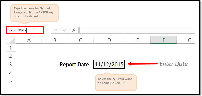
Creating Names With The «Name Manager»
If you want to customize your named ranges even more, you can open up the Name Manager (Formulas tab > Defined Names group > Name Manager button) to edit and create new named ranges.
I won’t go into great detail in this article, but know that with the Name Manager you can
-
Change the name of an existing Named Range
-
Change the reference formula
-
Specify the scope (what worksheets the name can be accessed from)
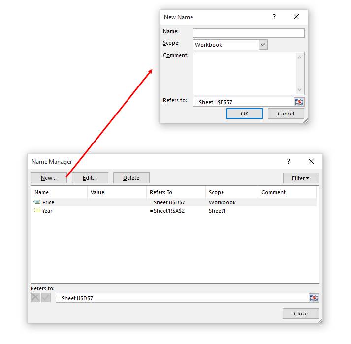
On To The VBA
Now that you have had a brief overview on Named Ranges, lets dig into some VBA macros you can use to help automate the use of Named Ranges.
Add A Named Range
The below VBA code shows ways you can create various types of named ranges.
Sub NameRange_Add()
‘PURPOSE: Various ways to create a Named Range
‘SOURCE: www.TheSpreadsheetGuru.com
Dim cell As Range
Dim rng As Range
Dim RangeName As String
Dim CellName As String
‘Single Cell Reference (Workbook Scope)
RangeName = «Price»
CellName = «D7»
Set cell = Worksheets(«Sheet1»).Range(CellName)
ThisWorkbook.Names.Add Name:=RangeName, RefersTo:=cell
‘Single Cell Reference (Worksheet Scope)
RangeName = «Year»
CellName = «A2»
Set cell = Worksheets(«Sheet1»).Range(CellName)
Worksheets(«Sheet1»).Names.Add Name:=RangeName, RefersTo:=cell
‘Range of Cells Reference (Workbook Scope)
RangeName = «myData»
CellName = «F9:J18»
Set cell = Worksheets(«Sheet1»).Range(CellName)
ThisWorkbook.Names.Add Name:=RangeName, RefersTo:=cell
‘Secret Named Range (doesn’t show up in Name Manager)
RangeName = «Username»
CellName = «L45»
Set cell = Worksheets(«Sheet1»).Range(CellName)
ThisWorkbook.Names.Add Name:=RangeName, RefersTo:=cell, Visible:=False
End Sub
Loop Through Named Ranges
This VBA macro code shows how you can cycle through the named ranges within your spreadsheet.
Sub NamedRange_Loop()
‘PURPOSE: Delete all Named Ranges in the Active Workbook
‘SOURCE: www.TheSpreadsheetGuru.com
Dim nm As Name
‘Loop through each named range in workbook
For Each nm In ActiveWorkbook.Names
Debug.Print nm.Name, nm.RefersTo
Next nm
‘Loop through each named range scoped to a specific worksheet
For Each nm In Worksheets(«Sheet1»).Names
Debug.Print nm.Name, nm.RefersTo
Next nm
End Sub
Delete All Named Ranges
If you need to clean up a bunch of junk named ranges, this VBA code will let you do it.
Sub NamedRange_DeleteAll()
‘PURPOSE: Delete all Named Ranges in the ActiveWorkbook (Print Areas optional)
‘SOURCE: www.TheSpreadsheetGuru.com
Dim nm As Name
Dim DeleteCount As Long
‘Delete PrintAreas as well?
UserAnswer = MsgBox(«Do you want to skip over Print Areas?», vbYesNoCancel)
If UserAnswer = vbYes Then SkipPrintAreas = True
If UserAnswer = vbCancel Then Exit Sub
‘Error Handler in case Delete Function Errors out
On Error GoTo Skip
‘Loop through each name and delete
For Each nm In ActiveWorkbook.Names
If SkipPrintAreas = True And Right(nm.Name, 10) = «Print_Area» Then GoTo Skip
‘Error Handler in case Delete Function Errors out
On Error GoTo Skip
‘Delete Named Range
nm.Delete
DeleteCount = DeleteCount + 1
Skip:
‘Reset Error Handler
On Error GoTo 0
Next
‘Report Result
If DeleteCount = 1 Then
MsgBox «[1] name was removed from this workbook.»
Else
MsgBox «[» & DeleteCount & «] names were removed from this workbook.»
End If
End Sub
Delete Named Ranges with Error References
This VBA code will delete only Named Ranges with errors in them. These errors can be caused by worksheets being deleted or rows/columns being deleted.
Sub NamedRange_DeleteErrors()
‘PURPOSE: Delete all Named Ranges with #REF error in the ActiveWorkbook
‘SOURCE: www.TheSpreadsheetGuru.com
Dim nm As Name
Dim DeleteCount As Long
‘Loop through each name and delete
For Each nm In ActiveWorkbook.Names
If InStr(1, nm.RefersTo, «#REF!») > 0 Then
‘Error Handler in case Delete Function Errors out
On Error GoTo Skip
‘Delete Named Range
nm.Delete
DeleteCount = DeleteCount + 1
End If
Skip:
‘Reset Error Handler
On Error GoTo 0
Next
‘Report Result
If DeleteCount = 1 Then
MsgBox «[1] errorant name was removed from this workbook.»
Else
MsgBox «[» & DeleteCount & «] errorant names were removed from this workbook.»
End If
End Sub
Anything Missing From This Guide?
Let me know if you have any ideas for other useful VBA macros concerning Named Ranges. Or better yet, share with me your own macros and I can add them to the article for everyone else to see! I look forward to reading your comments below.
About The Author
Hey there! I’m Chris and I run TheSpreadsheetGuru website in my spare time. By day, I’m actually a finance professional who relies on Microsoft Excel quite heavily in the corporate world. I love taking the things I learn in the “real world” and sharing them with everyone here on this site so that you too can become a spreadsheet guru at your company.
Through my years in the corporate world, I’ve been able to pick up on opportunities to make working with Excel better and have built a variety of Excel add-ins, from inserting tickmark symbols to automating copy/pasting from Excel to PowerPoint. If you’d like to keep up to date with the latest Excel news and directly get emailed the most meaningful Excel tips I’ve learned over the years, you can sign up for my free newsletters. I hope I was able to provide you with some value today and I hope to see you back here soon!
— Chris
Founder, TheSpreadsheetGuru.com