
In this article, we will be dealing with the conversion of Excel (.xlsx) file into .csv. There are two formats mostly used in Excel :
- (*.xlsx) : Excel Microsoft Office Open XML Format Spreadsheet file.
- (*.xls) : Excel Spreadsheet (Excel 97-2003 workbook).
Let’s Consider a dataset of a shopping store having data about Customer Serial Number, Customer Name, Customer ID, and Product Cost stored in Excel file.
check all used files here.
Python3
import pandas as pd
df = pd.DataFrame(pd.read_excel("Test.xlsx"))
df
Output :

Now, let’s see different ways to convert an Excel file into a CSV file :
Method 1: Convert Excel file to CSV file using the pandas library.
Pandas is an open-source software library built for data manipulation and analysis for Python programming language. It offers various functionality in terms of data structures and operations for manipulating numerical tables and time series. It can read, filter, and re-arrange small and large datasets and output them in a range of formats including Excel, JSON, CSV.
For reading an excel file, using the read_excel() method and convert the data frame into the CSV file, use to_csv() method of pandas.
Code:
Python3
import pandas as pd
read_file = pd.read_excel ("Test.xlsx")
read_file.to_csv ("Test.csv",
index = None,
header=True)
df = pd.DataFrame(pd.read_csv("Test.csv"))
df
Output:

Method 2: Convert Excel file to CSV file using xlrd and CSV library.
xlrd is a library with the main purpose to read an excel file.
csv is a library with the main purpose to read and write a csv file.
Code:
Python3
import xlrd
import csv
import pandas as pd
sheet = xlrd.open_workbook("Test.xlsx").sheet_by_index(0)
col = csv.writer(open("T.csv",
'w',
newline=""))
for row in range(sheet.nrows):
col.writerow(sheet.row_values(row))
df = pd.DataFrame(pd.read_csv("T.csv"))
df
Output:

Method 3: Convert Excel file to CSV file using openpyxl and CSV library.
openpyxl is a library to read/write Excel 2010 xlsx/xlsm/xltx/xltm files.It was born from lack of existing library to read/write natively from Python the Office Open XML format.
Code:
Python3
import openpyxl
import csv
import pandas as pd
excel = openpyxl.load_workbook("Test.xlsx")
sheet = excel.active
col = csv.writer(open("tt.csv",
'w',
newline=""))
for r in sheet.rows:
col.writerow([cell.value for cell in r])
df = pd.DataFrame(pd.read_csv("tt.csv"))
df
Output:

Время на прочтение
10 мин
Количество просмотров 290K
Первая часть статьи была опубликована тут.
Как читать и редактировать Excel файлы при помощи openpyxl
ПЕРЕВОД
Оригинал статьи — www.datacamp.com/community/tutorials/python-excel-tutorial
Автор — Karlijn Willems
Эта библиотека пригодится, если вы хотите читать и редактировать файлы .xlsx, xlsm, xltx и xltm.
Установите openpyxl using pip. Общие рекомендации по установке этой библиотеки — сделать это в виртуальной среде Python без системных библиотек. Вы можете использовать виртуальную среду для создания изолированных сред Python: она создает папку, содержащую все необходимые файлы, для использования библиотек, которые потребуются для Python.
Перейдите в директорию, в которой находится ваш проект, и повторно активируйте виртуальную среду venv. Затем перейдите к установке openpyxl с помощью pip, чтобы убедиться, что вы можете читать и записывать с ним файлы:
# Activate virtualenv
$ source activate venv

# Install `openpyxl` in `venv`
$ pip install openpyxl
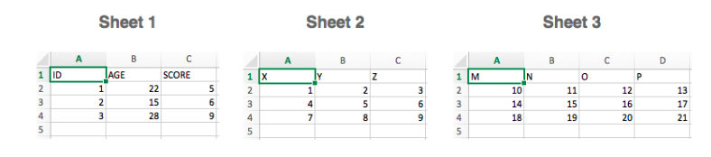
Теперь, когда вы установили openpyxl, вы можете начать загрузку данных. Но что именно это за данные? Например, в книге с данными, которые вы пытаетесь получить на Python, есть следующие листы:
Функция load_workbook () принимает имя файла в качестве аргумента и возвращает объект рабочей книги, который представляет файл. Это можно проверить запуском type (wb). Не забудьте убедиться, что вы находитесь в правильной директории, где расположена электронная таблица. В противном случае вы получите сообщение об ошибке при импорте.
# Import `load_workbook` module from `openpyxl`
from openpyxl import load_workbook

# Load in the workbook
wb = load_workbook('./test.xlsx')

# Get sheet names
print(wb.get_sheet_names())
Помните, вы можете изменить рабочий каталог с помощью os.chdir (). Фрагмент кода выше возвращает имена листов книги, загруженной в Python. Вы можете использовать эту информацию для получения отдельных листов книги. Также вы можете проверить, какой лист активен в настоящий момент с помощью wb.active. В приведенном ниже коде, вы также можете использовать его для загрузки данных на другом листе книги:
# Get a sheet by name
sheet = wb.get_sheet_by_name('Sheet3')

# Print the sheet title
sheet.title

# Get currently active sheet
anotherSheet = wb.active

# Check `anotherSheet`
anotherSheet
На первый взгляд, с этими объектами Worksheet мало что можно сделать. Однако, можно извлекать значения из определенных ячеек на листе книги, используя квадратные скобки [], к которым нужно передавать точную ячейку, из которой вы хотите получить значение.
Обратите внимание, это похоже на выбор, получение и индексирование массивов NumPy и Pandas DataFrames, но это еще не все, что нужно сделать, чтобы получить значение. Нужно еще добавить значение атрибута:
# Retrieve the value of a certain cell
sheet['A1'].value

# Select element 'B2' of your sheet
c = sheet['B2']

# Retrieve the row number of your element
c.row

# Retrieve the column letter of your element
c.column

# Retrieve the coordinates of the cell
c.coordinate
Помимо value, есть и другие атрибуты, которые можно использовать для проверки ячейки, а именно row, column и coordinate:
Атрибут row вернет 2;
Добавление атрибута column к “С” даст вам «B»;
coordinate вернет «B2».
Вы также можете получить значения ячеек с помощью функции cell (). Передайте аргументы row и column, добавьте значения к этим аргументам, которые соответствуют значениям ячейки, которые вы хотите получить, и, конечно же, не забудьте добавить атрибут value:
# Retrieve cell value
sheet.cell(row=1, column=2).value

# Print out values in column 2
for i in range(1, 4):
     print(i, sheet.cell(row=i, column=2).value)
Обратите внимание: если вы не укажете значение атрибута value, вы получите <Cell Sheet3.B1>, который ничего не говорит о значении, которое содержится в этой конкретной ячейке.
Вы используете цикл с помощью функции range (), чтобы помочь вам вывести значения строк, которые имеют значения в столбце 2. Если эти конкретные ячейки пусты, вы получите None.
Более того, существуют специальные функции, которые вы можете вызвать, чтобы получить другие значения, например get_column_letter () и column_index_from_string.
В двух функциях уже более или менее указано, что вы можете получить, используя их. Но лучше всего сделать их явными: пока вы можете получить букву прежнего столбца, можно сделать обратное или получить индекс столбца, перебирая букву за буквой. Как это работает:
# Import relevant modules from `openpyxl.utils`
from openpyxl.utils import get_column_letter, column_index_from_string

# Return 'A'
get_column_letter(1)

# Return '1'
column_index_from_string('A')
Вы уже получили значения для строк, которые имеют значения в определенном столбце, но что нужно сделать, если нужно вывести строки файла, не сосредотачиваясь только на одном столбце?
Конечно, использовать другой цикл.
Например, вы хотите сосредоточиться на области, находящейся между «A1» и «C3», где первый указывает левый верхний угол, а второй — правый нижний угол области, на которой вы хотите сфокусироваться. Эта область будет так называемой cellObj, которую вы видите в первой строке кода ниже. Затем вы указываете, что для каждой ячейки, которая находится в этой области, вы хотите вывести координату и значение, которое содержится в этой ячейке. После окончания каждой строки вы хотите выводить сообщение-сигнал о том, что строка этой области cellObj была выведена.
# Print row per row
for cellObj in sheet['A1':'C3']:
      for cell in cellObj:
              print(cells.coordinate, cells.value)
      print('--- END ---')
Обратите внимание, что выбор области очень похож на выбор, получение и индексирование списка и элементы NumPy, где вы также используете квадратные скобки и двоеточие чтобы указать область, из которой вы хотите получить значения. Кроме того, вышеприведенный цикл также хорошо использует атрибуты ячейки!
Чтобы визуализировать описанное выше, возможно, вы захотите проверить результат, который вернет вам завершенный цикл:
('A1', u'M')
('B1', u'N')
('C1', u'O')
--- END ---
('A2', 10L)
('B2', 11L)
('C2', 12L)
--- END ---
('A3', 14L)
('B3', 15L)
('C3', 16L)
--- END ---
Наконец, есть некоторые атрибуты, которые вы можете использовать для проверки результата импорта, а именно max_row и max_column. Эти атрибуты, конечно, являются общими способами обеспечения правильной загрузки данных, но тем не менее в данном случае они могут и будут полезны.
# Retrieve the maximum amount of rows
sheet.max_row

# Retrieve the maximum amount of columns
sheet.max_column
Это все очень классно, но мы почти слышим, что вы сейчас думаете, что это ужасно трудный способ работать с файлами, особенно если нужно еще и управлять данными.
Должно быть что-то проще, не так ли? Всё так!
Openpyxl имеет поддержку Pandas DataFrames. И можно использовать функцию DataFrame () из пакета Pandas, чтобы поместить значения листа в DataFrame:
# Import `pandas`
import pandas as pd

# Convert Sheet to DataFrame
df = pd.DataFrame(sheet.values)
Если вы хотите указать заголовки и индексы, вам нужно добавить немного больше кода:
# Put the sheet values in `data`
data = sheet.values

# Indicate the columns in the sheet values
cols = next(data)[1:]

# Convert your data to a list
data = list(data)

# Read in the data at index 0 for the indices
idx = [r[0] for r in data]

# Slice the data at index 1
data = (islice(r, 1, None) for r in data)

# Make your DataFrame
df = pd.DataFrame(data, index=idx, columns=cols)
Затем вы можете начать управлять данными при помощи всех функций, которые есть в Pandas. Но помните, что вы находитесь в виртуальной среде, поэтому, если библиотека еще не подключена, вам нужно будет установить ее снова через pip.
Чтобы записать Pandas DataFrames обратно в файл Excel, можно использовать функцию dataframe_to_rows () из модуля utils:
# Import `dataframe_to_rows`
from openpyxl.utils.dataframe import dataframe_to_rows

# Initialize a workbook
wb = Workbook()

# Get the worksheet in the active workbook
ws = wb.active

# Append the rows of the DataFrame to your worksheet
for r in dataframe_to_rows(df, index=True, header=True):
    ws.append(r)
Но это определенно не все! Библиотека openpyxl предлагает вам высокую гибкость в отношении того, как вы записываете свои данные в файлы Excel, изменяете стили ячеек или используете режим только для записи. Это делает ее одной из тех библиотек, которую вам точно необходимо знать, если вы часто работаете с электронными таблицами.
И не забудьте деактивировать виртуальную среду, когда закончите работу с данными!
Теперь давайте рассмотрим некоторые другие библиотеки, которые вы можете использовать для получения данных в электронной таблице на Python.
Готовы узнать больше?
Чтение и форматирование Excel файлов xlrd
Эта библиотека идеальна, если вы хотите читать данные и форматировать данные в файлах с расширением .xls или .xlsx.
# Import `xlrd`
import xlrd

# Open a workbook
workbook = xlrd.open_workbook('example.xls')

# Loads only current sheets to memory
workbook = xlrd.open_workbook('example.xls', on_demand = True)
Если вы не хотите рассматривать всю книгу, можно использовать такие функции, как sheet_by_name () или sheet_by_index (), чтобы извлекать листы, которые необходимо использовать в анализе.
# Load a specific sheet by name
worksheet = workbook.sheet_by_name('Sheet1')

# Load a specific sheet by index
worksheet = workbook.sheet_by_index(0)

# Retrieve the value from cell at indices (0,0)
sheet.cell(0, 0).value
Наконец, можно получить значения по определенным координатам, обозначенным индексами.
О том, как xlwt и xlutils, соотносятся с xlrd расскажем дальше.
Запись данных в Excel файл при помощи xlrd
Если нужно создать электронные таблицы, в которых есть данные, кроме библиотеки XlsxWriter можно использовать библиотеки xlwt. Xlwt идеально подходит для записи и форматирования данных в файлы с расширением .xls.
Когда вы вручную хотите записать в файл, это будет выглядеть так:
# Import `xlwt`
import xlwt
# Initialize a workbook
book = xlwt.Workbook(encoding="utf-8")
# Add a sheet to the workbook
sheet1 = book.add_sheet("Python Sheet 1")
# Write to the sheet of the workbook
sheet1.write(0, 0, "This is the First Cell of the First Sheet")
# Save the workbook
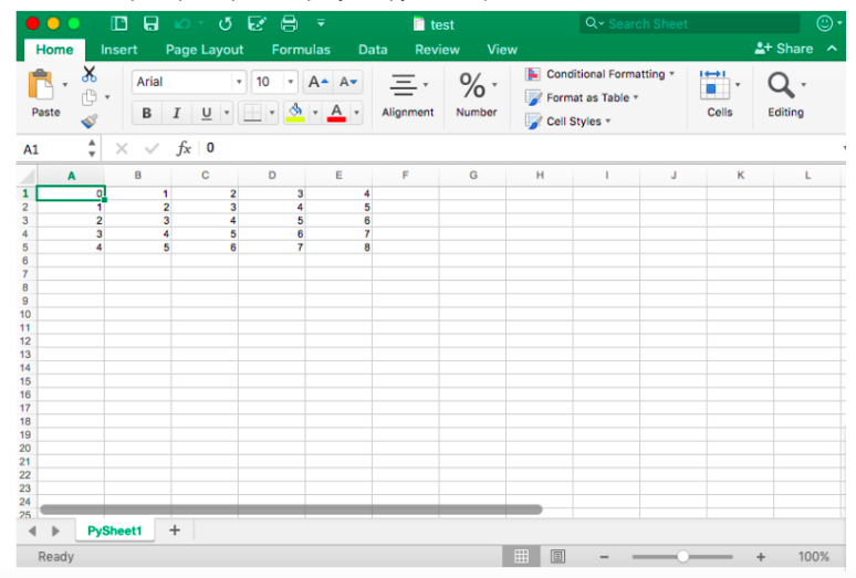
book.save("spreadsheet.xls")Если нужно записать данные в файл, то для минимизации ручного труда можно прибегнуть к циклу for. Это позволит немного автоматизировать процесс. Делаем скрипт, в котором создается книга, в которую добавляется лист. Далее указываем список со столбцами и со значениями, которые будут перенесены на рабочий лист.
Цикл for будет следить за тем, чтобы все значения попадали в файл: задаем, что с каждым элементом в диапазоне от 0 до 4 (5 не включено) мы собираемся производить действия. Будем заполнять значения строка за строкой. Для этого указываем row элемент, который будет “прыгать” в каждом цикле. А далее у нас следующий for цикл, который пройдется по столбцам листа. Задаем условие, что для каждой строки на листе смотрим на столбец и заполняем значение для каждого столбца в строке. Когда заполнили все столбцы строки значениями, переходим к следующей строке, пока не заполним все имеющиеся строки.
# Initialize a workbook
book = xlwt.Workbook()

# Add a sheet to the workbook
sheet1 = book.add_sheet("Sheet1")

# The data
cols = ["A", "B", "C", "D", "E"]
txt = [0,1,2,3,4]

# Loop over the rows and columns and fill in the values
for num in range(5):
      row = sheet1.row(num)
      for index, col in enumerate(cols):
          value = txt[index] + num
          row.write(index, value)

# Save the result
book.save("test.xls")
В качестве примера скриншот результирующего файла:
Теперь, когда вы видели, как xlrd и xlwt взаимодействуют вместе, пришло время посмотреть на библиотеку, которая тесно связана с этими двумя: xlutils.
Коллекция утилит xlutils
Эта библиотека в основном представляет собой набор утилит, для которых требуются как xlrd, так и xlwt. Включает в себя возможность копировать и изменять/фильтровать существующие файлы. Вообще говоря, оба этих случая подпадают теперь под openpyxl.
Использование pyexcel для чтения файлов .xls или .xlsx
Еще одна библиотека, которую можно использовать для чтения данных таблиц в Python — pyexcel. Это Python Wrapper, который предоставляет один API для чтения, обработки и записи данных в файлах .csv, .ods, .xls, .xlsx и .xlsm.
Чтобы получить данные в массиве, можно использовать функцию get_array (), которая содержится в пакете pyexcel:
# Import `pyexcel`
import pyexcel

# Get an array from the data
my_array = pyexcel.get_array(file_name="test.xls")

Также можно получить данные в упорядоченном словаре списков, используя функцию get_dict ():
# Import `OrderedDict` module
from pyexcel._compact import OrderedDict

# Get your data in an ordered dictionary of lists
my_dict = pyexcel.get_dict(file_name="test.xls", name_columns_by_row=0)

# Get your data in a dictionary of 2D arrays
book_dict = pyexcel.get_book_dict(file_name="test.xls")
Однако, если вы хотите вернуть в словарь двумерные массивы или, иными словами, получить все листы книги в одном словаре, стоит использовать функцию get_book_dict ().
Имейте в виду, что обе упомянутые структуры данных, массивы и словари вашей электронной таблицы, позволяют создавать DataFrames ваших данных с помощью pd.DataFrame (). Это упростит обработку ваших данных!
Наконец, вы можете просто получить записи с pyexcel благодаря функции get_records (). Просто передайте аргумент file_name функции и обратно получите список словарей:
# Retrieve the records of the file
records = pyexcel.get_records(file_name="test.xls")
Записи файлов при помощи pyexcel
Так же, как загрузить данные в массивы с помощью этого пакета, можно также легко экспортировать массивы обратно в электронную таблицу. Для этого используется функция save_as () с передачей массива и имени целевого файла в аргумент dest_file_name:
# Get the data
data = [[1, 2, 3], [4, 5, 6], [7, 8, 9]]

# Save the array to a file
pyexcel.save_as(array=data, dest_file_name="array_data.xls")
Обратите внимание: если указать разделитель, то можно добавить аргумент dest_delimiter и передать символ, который хотите использовать, в качестве разделителя между “”.
Однако, если у вас есть словарь, нужно будет использовать функцию save_book_as (). Передайте двумерный словарь в bookdict и укажите имя файла, и все ОК:
# The data
2d_array_dictionary = {'Sheet 1': [
                                   ['ID', 'AGE', 'SCORE']
                                   [1, 22, 5],
                                   [2, 15, 6],
                                   [3, 28, 9]
                                  ],
                       'Sheet 2': [
                                    ['X', 'Y', 'Z'],
                                    [1, 2, 3],
                                    [4, 5, 6]
                                    [7, 8, 9]
                                  ],
                       'Sheet 3': [
                                    ['M', 'N', 'O', 'P'],
                                    [10, 11, 12, 13],
                                    [14, 15, 16, 17]
                                    [18, 19, 20, 21]
                                   ]}

# Save the data to a file
pyexcel.save_book_as(bookdict=2d_array_dictionary, dest_file_name="2d_array_data.xls")
Помните, что когда используете код, который напечатан в фрагменте кода выше, порядок данных в словаре не будет сохранен!
Чтение и запись .csv файлов
Если вы все еще ищете библиотеки, которые позволяют загружать и записывать данные в CSV-файлы, кроме Pandas, рекомендуем библиотеку csv:
# import `csv`
import csv

# Read in csv file
for row in csv.reader(open('data.csv'), delimiter=','):
      print(row)

# Write csv file
data = [[1, 2, 3], [4, 5, 6], [7, 8, 9]]
outfile = open('data.csv', 'w')
writer = csv.writer(outfile, delimiter=';', quotechar='"')
writer.writerows(data)
outfile.close()
Обратите внимание, что NumPy имеет функцию genfromtxt (), которая позволяет загружать данные, содержащиеся в CSV-файлах в массивах, которые затем можно помещать в DataFrames.
Финальная проверка данных
Когда данные подготовлены, не забудьте последний шаг: проверьте правильность загрузки данных. Если вы поместили свои данные в DataFrame, вы можете легко и быстро проверить, был ли импорт успешным, выполнив следующие команды:
# Check the first entries of the DataFrame
df1.head()

# Check the last entries of the DataFrame
df1.tail()
Note: Используйте DataCamp Pandas Cheat Sheet, когда вы планируете загружать файлы в виде Pandas DataFrames.
Если данные в массиве, вы можете проверить его, используя следующие атрибуты массива: shape, ndim, dtype и т.д.:
# Inspect the shape
data.shape

# Inspect the number of dimensions
data.ndim

# Inspect the data type
data.dtype
Что дальше?
Поздравляем, теперь вы знаете, как читать файлы Excel в Python  Но импорт данных — это только начало рабочего процесса в области данных. Когда у вас есть данные из электронных таблиц в вашей среде, вы можете сосредоточиться на том, что действительно важно: на анализе данных.
Если вы хотите глубже погрузиться в тему — знакомьтесь с PyXll, которая позволяет записывать функции в Python и вызывать их в Excel.

This article will show in detail how to work with Excel files and how to modify specific data with Python.
First we will learn how to work with CSV files by reading, writing and updating them. Then we will take a look how to read files, filter them by sheets, search for rows/columns, and update cells of xlsx files.
Let’s start with the simplest spreadsheet format: CSV.
Part 1 — The CSV file
A CSV file is a comma-separated values file, where plain text data is displayed in a tabular format. They can be used with any spreadsheet program, such as Microsoft Office Excel, Google Spreadsheets, or LibreOffice Calc.
CSV files are not like other spreadsheet files though, because they don’t allow you to save cells, columns, rows or formulas. Their limitation is that they also allow only one sheet per file. My plan for this first part of the article is to show you how to create CSV files using Python 3 and the standard library module CSV.
This tutorial will end with two GitHub repositories and a live web application that actually uses the code of the second part of this tutorial (yet updated and modified to be for a specific purpose).
Writing to CSV files
First, open a new Python file and import the Python CSV module.
import csvCSV Module
The CSV module includes all the necessary methods built in. These include:
- csv.reader
- csv.writer
- csv.DictReader
- csv.DictWriter
- and others
In this guide we are going to focus on the writer, DictWriter and DictReader methods. These allow you to edit, modify, and manipulate the data stored in a CSV file.
In the first step we need to define the name of the file and save it as a variable. We should do the same with the header and data information.
filename = "imdb_top_4.csv"
header = ("Rank", "Rating", "Title")
data = [
(1, 9.2, "The Shawshank Redemption(1994)"),
(2, 9.2, "The Godfather(1972)"),
(3, 9, "The Godfather: Part II(1974)"),
(4, 8.9, "Pulp Fiction(1994)")
]
Now we need to create a function named writer that will take in three parameters: header, data and filename.
def writer(header, data, filename):
  pass
The next step is to modify the writer function so it creates a file that holds data from the header and data variables. This is done by writing the first row from the header variable and then writing four rows from the data variable (there are four rows because there are four tuples inside the list).
def writer(header, data, filename):
  with open (filename, "w", newline = "") as csvfile:
    movies = csv.writer(csvfile)
    movies.writerow(header)
    for x in data:
      movies.writerow(x)
The official Python documentation describes how the csv.writer method works. I would strongly suggest that you to take a minute to read it.
And voilà! You created your first CSV file named imdb_top_4.csv. Open this file with your preferred spreadsheet application and you should see something like this:
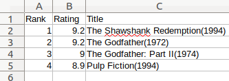
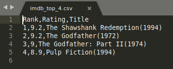
The result might be written like this if you choose to open the file in some other application:
Updating the CSV files
To update this file you should create a new function named updater that will take just one parameter called filename.
def updater(filename):
    with open(filename, newline= "") as file:
        readData = [row for row in csv.DictReader(file)]
        # print(readData)
        readData[0]['Rating'] = '9.4'
        # print(readData)

    readHeader = readData[0].keys()
    writer(readHeader, readData, filename, "update")
This function first opens the file defined in the filename variable and then saves all the data it reads from the file inside of a variable named readData. The second step is to hard code the new value and place it instead of the old one in the readData[0][‘Rating’] position.
The last step in the function is to call the writer function by adding a new parameter update that will tell the function that you are doing an update.
csv.DictReader is explained more in the official Python documentation here.
For writer to work with a new parameter, you need to add a new parameter everywhere writer is defined. Go back to the place where you first called the writer function and add “write” as a new parameter:
writer(header, data, filename, "write")Just below the writer function call the updater and pass the filename parameter into it:
writer(header, data, filename, "write")
updater(filename)
Now you need to modify the writer function to take a new parameter named option:
def writer(header, data, filename, option):From now on we expect to receive two different options for the writer function (write and update). Because of that we should add two if statements to support this new functionality. First part of the function under “if option == “write:” is already known to you. You just need to add the “elif option == “update”: section of the code and the else part just as they are written bellow:
def writer(header, data, filename, option):
        with open (filename, "w", newline = "") as csvfile:
            if option == "write":

                movies = csv.writer(csvfile)
                movies.writerow(header)
                for x in data:
                    movies.writerow(x)
            elif option == "update":
                writer = csv.DictWriter(csvfile, fieldnames = header)
                writer.writeheader()
                writer.writerows(data)
            else:
                print("Option is not known")
Bravo! Your are done!
Now your code should look something like this:
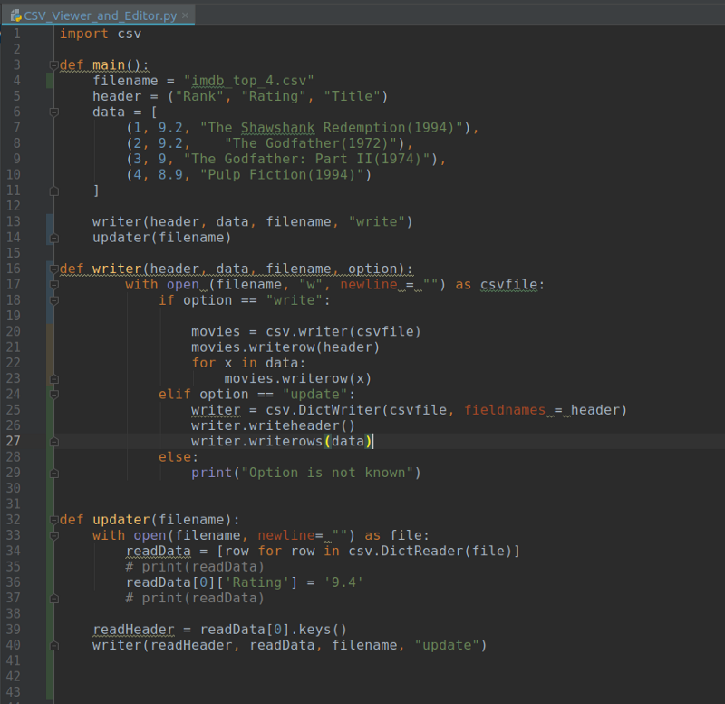
You can also find the code here:
https://github.com/GoranAviani/CSV-Viewer-and-Editor
In the first part of this article we have seen how to work with CSV files. We have created and updated one such file.
Part 2 — The xlsx file
For several weekends I have worked on this project. I have started working on it because there was a need for this kind of solution in my company. My first idea was to build this solution directly in my company’s system, but then I wouldn’t have anything to write about, eh?
I build this solution using Python 3 and openpyxl library. The reason why I have chosen openpyxl is because it represents a complete solution for creating worksheets, loading, updating, renaming and deleting them. It also allows us to read or write to rows and columns, merge or un-merge cells or create Python excel charts etc.
Openpyxl terminology and basic info
- Workbook is the name for an Excel file in Openpyxl.
- A workbook consists of sheets (default is 1 sheet). Sheets are referenced by their names.
- A sheet consists of rows (horizontal lines) starting from the number 1 and columns (vertical lines) starting from the letter A.
- Rows and columns result in a grid and form cells which may contain some data (numerical or string value) or formulas.
Openpyxl in nicely documented and I would advise that you take a look here.
The first step is to open your Python environment and install openpyxl within your terminal:
pip install openpyxlNext, import openpyxl into your project and then to load a workbook into the theFile variable.
import openpyxl

theFile = openpyxl.load_workbook('Customers1.xlsx')
print(theFile.sheetnames)
currentSheet = theFile['customers 1']
print(currentSheet['B4'].value)
As you can see, this code prints all sheets by their names. It then selects the sheet that is named “customers 1” and saves it to a currentSheet variable. In the last line, the code prints the value that is located in the B4 position of the “customers 1” sheet.
This code works as it should but it is very hard coded. To make this more dynamic we will write code that will:
- Read the file
- Get all sheet names
- Loop through all sheets
- In the last step, the code will print values that are located in B4 fields of each found sheet inside the workbook.
import openpyxl

theFile = openpyxl.load_workbook('Customers1.xlsx')
allSheetNames = theFile.sheetnames

print("All sheet names {} " .format(theFile.sheetnames))


for x in allSheetNames:
    print("Current sheet name is {}" .format(x))
    currentSheet = theFile[x]
    print(currentSheet['B4'].value)
This is better than before, but it is still a hard coded solution and it still assumes the value you will be looking for is in the B4 cell, which is just silly
I expect your project will need to search inside all sheets in the Excel file for a specific value. To do this we will add one more for loop in the “ABCDEF” range and then simply print cell names and their values.
import openpyxl

theFile = openpyxl.load_workbook('Customers1.xlsx')
allSheetNames = theFile.sheetnames

print("All sheet names {} " .format(theFile.sheetnames))


for sheet in allSheetNames:
    print("Current sheet name is {}" .format(sheet))
    currentSheet = theFile[sheet]
    # print(currentSheet['B4'].value)

    #print max numbers of wors and colums for each sheet
    #print(currentSheet.max_row)
    #print(currentSheet.max_column)

    for row in range(1, currentSheet.max_row + 1):
        #print(row)
        for column in "ABCDEF":  # Here you can add or reduce the columns
            cell_name = "{}{}".format(column, row)
            #print(cell_name)
            print("cell position {} has value {}".format(cell_name, currentSheet[cell_name].value))
We did this by introducing the “for row in range..” loop. The range of the for loop is defined from the cell in row 1 to the sheet’s maximum number or rows. The second for loop searches within predefined column names “ABCDEF”. In the second loop we will display the full position of the cell (column name and row number) and a value.
However, in this article my task is to find a specific column that is named “telephone” and then go through all the rows of that column. To do that we need to modify the code like below.
import openpyxl

theFile = openpyxl.load_workbook('Customers1.xlsx')
allSheetNames = theFile.sheetnames

print("All sheet names {} " .format(theFile.sheetnames))


def find_specific_cell():
    for row in range(1, currentSheet.max_row + 1):
        for column in "ABCDEFGHIJKL":  # Here you can add or reduce the columns
            cell_name = "{}{}".format(column, row)
            if currentSheet[cell_name].value == "telephone":
                #print("{1} cell is located on {0}" .format(cell_name, currentSheet[cell_name].value))
                print("cell position {} has value {}".format(cell_name, currentSheet[cell_name].value))
                return cell_name

for sheet in allSheetNames:
    print("Current sheet name is {}" .format(sheet))
    currentSheet = theFile[sheet]
This modified code goes through all cells of every sheet, and just like before the row range is dynamic and the column range is specific. The code loops through cells and looks for a cell that holds a text “telephone”. Once the code finds the specific cell it notifies the user in which cell the text is located. The code does this for every cell inside of all sheets that are in the Excel file.
The next step is to go through all rows of that specific column and print values.
import openpyxl

theFile = openpyxl.load_workbook('Customers1.xlsx')
allSheetNames = theFile.sheetnames

print("All sheet names {} " .format(theFile.sheetnames))


def find_specific_cell():
    for row in range(1, currentSheet.max_row + 1):
        for column in "ABCDEFGHIJKL":  # Here you can add or reduce the columns
            cell_name = "{}{}".format(column, row)
            if currentSheet[cell_name].value == "telephone":
                #print("{1} cell is located on {0}" .format(cell_name, currentSheet[cell_name].value))
                print("cell position {} has value {}".format(cell_name, currentSheet[cell_name].value))
                return cell_name

def get_column_letter(specificCellLetter):
    letter = specificCellLetter[0:-1]
    print(letter)
    return letter

def get_all_values_by_cell_letter(letter):
    for row in range(1, currentSheet.max_row + 1):
        for column in letter:
            cell_name = "{}{}".format(column, row)
            #print(cell_name)
            print("cell position {} has value {}".format(cell_name, currentSheet[cell_name].value))


for sheet in allSheetNames:
    print("Current sheet name is {}" .format(sheet))
    currentSheet = theFile[sheet]
    specificCellLetter = (find_specific_cell())
    letter = get_column_letter(specificCellLetter)

    get_all_values_by_cell_letter(letter)
This is done by adding a function named get_column_letter that finds a letter of a column. After the letter of the column is found we loop through all rows of that specific column. This is done with the get_all_values_by_cell_letter function which will print all values of those cells.
Wrapping up
Bra gjort! There are many thing you can do after this. My plan was to build an online app that will standardize all Swedish telephone numbers taken from a text box and offer users the possibility to simply copy the results from the same text box. The second step of my plan was to expand the functionality of the web app to support the upload of Excel files, processing of telephone numbers inside those files (standardizing them to a Swedish format) and offering the processed files back to users.
I have done both of those tasks and you can see them live in the Tools page of my Incodaq.com site:
https://tools.incodaq.com/
Also the code from the second part of this article is available on GitHub:
https://github.com/GoranAviani/Manipulate-Excel-spreadsheets
Thank you for reading! Check out more articles like this on my Medium profile: https://medium.com/@goranaviani and other fun stuff I build on my GitHub page: https://github.com/GoranAviani
Learn to code for free. freeCodeCamp’s open source curriculum has helped more than 40,000 people get jobs as developers. Get started
Watch Now This tutorial has a related video course created by the Real Python team. Watch it together with the written tutorial to deepen your understanding: Reading and Writing Files With Pandas
pandas is a powerful and flexible Python package that allows you to work with labeled and time series data. It also provides statistics methods, enables plotting, and more. One crucial feature of pandas is its ability to write and read Excel, CSV, and many other types of files. Functions like the pandas read_csv() method enable you to work with files effectively. You can use them to save the data and labels from pandas objects to a file and load them later as pandas Series or DataFrame instances.
In this tutorial, you’ll learn:
- What the pandas IO tools API is
- How to read and write data to and from files
- How to work with various file formats
- How to work with big data efficiently
Let’s start reading and writing files!
Installing pandas
The code in this tutorial is executed with CPython 3.7.4 and pandas 0.25.1. It would be beneficial to make sure you have the latest versions of Python and pandas on your machine. You might want to create a new virtual environment and install the dependencies for this tutorial.
First, you’ll need the pandas library. You may already have it installed. If you don’t, then you can install it with pip:
Once the installation process completes, you should have pandas installed and ready.
Anaconda is an excellent Python distribution that comes with Python, many useful packages like pandas, and a package and environment manager called Conda. To learn more about Anaconda, check out Setting Up Python for Machine Learning on Windows.
If you don’t have pandas in your virtual environment, then you can install it with Conda:
Conda is powerful as it manages the dependencies and their versions. To learn more about working with Conda, you can check out the official documentation.
Preparing Data
In this tutorial, you’ll use the data related to 20 countries. Here’s an overview of the data and sources you’ll be working with:
-
Country is denoted by the country name. Each country is in the top 10 list for either population, area, or gross domestic product (GDP). The row labels for the dataset are the three-letter country codes defined in ISO 3166-1. The column label for the dataset is
COUNTRY. -
Population is expressed in millions. The data comes from a list of countries and dependencies by population on Wikipedia. The column label for the dataset is
POP. -
Area is expressed in thousands of kilometers squared. The data comes from a list of countries and dependencies by area on Wikipedia. The column label for the dataset is
AREA. -
Gross domestic product is expressed in millions of U.S. dollars, according to the United Nations data for 2017. You can find this data in the list of countries by nominal GDP on Wikipedia. The column label for the dataset is
GDP. -
Continent is either Africa, Asia, Oceania, Europe, North America, or South America. You can find this information on Wikipedia as well. The column label for the dataset is
CONT. -
Independence day is a date that commemorates a nation’s independence. The data comes from the list of national independence days on Wikipedia. The dates are shown in ISO 8601 format. The first four digits represent the year, the next two numbers are the month, and the last two are for the day of the month. The column label for the dataset is
IND_DAY.
This is how the data looks as a table:
| COUNTRY | POP | AREA | GDP | CONT | IND_DAY | |
|---|---|---|---|---|---|---|
| CHN | China | 1398.72 | 9596.96 | 12234.78 | Asia | |
| IND | India | 1351.16 | 3287.26 | 2575.67 | Asia | 1947-08-15 |
| USA | US | 329.74 | 9833.52 | 19485.39 | N.America | 1776-07-04 |
| IDN | Indonesia | 268.07 | 1910.93 | 1015.54 | Asia | 1945-08-17 |
| BRA | Brazil | 210.32 | 8515.77 | 2055.51 | S.America | 1822-09-07 |
| PAK | Pakistan | 205.71 | 881.91 | 302.14 | Asia | 1947-08-14 |
| NGA | Nigeria | 200.96 | 923.77 | 375.77 | Africa | 1960-10-01 |
| BGD | Bangladesh | 167.09 | 147.57 | 245.63 | Asia | 1971-03-26 |
| RUS | Russia | 146.79 | 17098.25 | 1530.75 | 1992-06-12 | |
| MEX | Mexico | 126.58 | 1964.38 | 1158.23 | N.America | 1810-09-16 |
| JPN | Japan | 126.22 | 377.97 | 4872.42 | Asia | |
| DEU | Germany | 83.02 | 357.11 | 3693.20 | Europe | |
| FRA | France | 67.02 | 640.68 | 2582.49 | Europe | 1789-07-14 |
| GBR | UK | 66.44 | 242.50 | 2631.23 | Europe | |
| ITA | Italy | 60.36 | 301.34 | 1943.84 | Europe | |
| ARG | Argentina | 44.94 | 2780.40 | 637.49 | S.America | 1816-07-09 |
| DZA | Algeria | 43.38 | 2381.74 | 167.56 | Africa | 1962-07-05 |
| CAN | Canada | 37.59 | 9984.67 | 1647.12 | N.America | 1867-07-01 |
| AUS | Australia | 25.47 | 7692.02 | 1408.68 | Oceania | |
| KAZ | Kazakhstan | 18.53 | 2724.90 | 159.41 | Asia | 1991-12-16 |
You may notice that some of the data is missing. For example, the continent for Russia is not specified because it spreads across both Europe and Asia. There are also several missing independence days because the data source omits them.
You can organize this data in Python using a nested dictionary:
data = {
    'CHN': {'COUNTRY': 'China', 'POP': 1_398.72, 'AREA': 9_596.96,
            'GDP': 12_234.78, 'CONT': 'Asia'},
    'IND': {'COUNTRY': 'India', 'POP': 1_351.16, 'AREA': 3_287.26,
            'GDP': 2_575.67, 'CONT': 'Asia', 'IND_DAY': '1947-08-15'},
    'USA': {'COUNTRY': 'US', 'POP': 329.74, 'AREA': 9_833.52,
            'GDP': 19_485.39, 'CONT': 'N.America',
            'IND_DAY': '1776-07-04'},
    'IDN': {'COUNTRY': 'Indonesia', 'POP': 268.07, 'AREA': 1_910.93,
            'GDP': 1_015.54, 'CONT': 'Asia', 'IND_DAY': '1945-08-17'},
    'BRA': {'COUNTRY': 'Brazil', 'POP': 210.32, 'AREA': 8_515.77,
            'GDP': 2_055.51, 'CONT': 'S.America', 'IND_DAY': '1822-09-07'},
    'PAK': {'COUNTRY': 'Pakistan', 'POP': 205.71, 'AREA': 881.91,
            'GDP': 302.14, 'CONT': 'Asia', 'IND_DAY': '1947-08-14'},
    'NGA': {'COUNTRY': 'Nigeria', 'POP': 200.96, 'AREA': 923.77,
            'GDP': 375.77, 'CONT': 'Africa', 'IND_DAY': '1960-10-01'},
    'BGD': {'COUNTRY': 'Bangladesh', 'POP': 167.09, 'AREA': 147.57,
            'GDP': 245.63, 'CONT': 'Asia', 'IND_DAY': '1971-03-26'},
    'RUS': {'COUNTRY': 'Russia', 'POP': 146.79, 'AREA': 17_098.25,
            'GDP': 1_530.75, 'IND_DAY': '1992-06-12'},
    'MEX': {'COUNTRY': 'Mexico', 'POP': 126.58, 'AREA': 1_964.38,
            'GDP': 1_158.23, 'CONT': 'N.America', 'IND_DAY': '1810-09-16'},
    'JPN': {'COUNTRY': 'Japan', 'POP': 126.22, 'AREA': 377.97,
            'GDP': 4_872.42, 'CONT': 'Asia'},
    'DEU': {'COUNTRY': 'Germany', 'POP': 83.02, 'AREA': 357.11,
            'GDP': 3_693.20, 'CONT': 'Europe'},
    'FRA': {'COUNTRY': 'France', 'POP': 67.02, 'AREA': 640.68,
            'GDP': 2_582.49, 'CONT': 'Europe', 'IND_DAY': '1789-07-14'},
    'GBR': {'COUNTRY': 'UK', 'POP': 66.44, 'AREA': 242.50,
            'GDP': 2_631.23, 'CONT': 'Europe'},
    'ITA': {'COUNTRY': 'Italy', 'POP': 60.36, 'AREA': 301.34,
            'GDP': 1_943.84, 'CONT': 'Europe'},
    'ARG': {'COUNTRY': 'Argentina', 'POP': 44.94, 'AREA': 2_780.40,
            'GDP': 637.49, 'CONT': 'S.America', 'IND_DAY': '1816-07-09'},
    'DZA': {'COUNTRY': 'Algeria', 'POP': 43.38, 'AREA': 2_381.74,
            'GDP': 167.56, 'CONT': 'Africa', 'IND_DAY': '1962-07-05'},
    'CAN': {'COUNTRY': 'Canada', 'POP': 37.59, 'AREA': 9_984.67,
            'GDP': 1_647.12, 'CONT': 'N.America', 'IND_DAY': '1867-07-01'},
    'AUS': {'COUNTRY': 'Australia', 'POP': 25.47, 'AREA': 7_692.02,
            'GDP': 1_408.68, 'CONT': 'Oceania'},
    'KAZ': {'COUNTRY': 'Kazakhstan', 'POP': 18.53, 'AREA': 2_724.90,
            'GDP': 159.41, 'CONT': 'Asia', 'IND_DAY': '1991-12-16'}
}

columns = ('COUNTRY', 'POP', 'AREA', 'GDP', 'CONT', 'IND_DAY')
Each row of the table is written as an inner dictionary whose keys are the column names and values are the corresponding data. These dictionaries are then collected as the values in the outer data dictionary. The corresponding keys for data are the three-letter country codes.
You can use this data to create an instance of a pandas DataFrame. First, you need to import pandas:
>>>
>>> import pandas as pd
Now that you have pandas imported, you can use the DataFrame constructor and data to create a DataFrame object.
data is organized in such a way that the country codes correspond to columns. You can reverse the rows and columns of a DataFrame with the property .T:
>>>
>>> df = pd.DataFrame(data=data).T
>>> df
        COUNTRY      POP     AREA      GDP       CONT     IND_DAY
CHN       China  1398.72  9596.96  12234.8       Asia         NaN
IND       India  1351.16  3287.26  2575.67       Asia  1947-08-15
USA          US   329.74  9833.52  19485.4  N.America  1776-07-04
IDN   Indonesia   268.07  1910.93  1015.54       Asia  1945-08-17
BRA      Brazil   210.32  8515.77  2055.51  S.America  1822-09-07
PAK    Pakistan   205.71   881.91   302.14       Asia  1947-08-14
NGA     Nigeria   200.96   923.77   375.77     Africa  1960-10-01
BGD  Bangladesh   167.09   147.57   245.63       Asia  1971-03-26
RUS      Russia   146.79  17098.2  1530.75        NaN  1992-06-12
MEX      Mexico   126.58  1964.38  1158.23  N.America  1810-09-16
JPN       Japan   126.22   377.97  4872.42       Asia         NaN
DEU     Germany    83.02   357.11   3693.2     Europe         NaN
FRA      France    67.02   640.68  2582.49     Europe  1789-07-14
GBR          UK    66.44    242.5  2631.23     Europe         NaN
ITA       Italy    60.36   301.34  1943.84     Europe         NaN
ARG   Argentina    44.94   2780.4   637.49  S.America  1816-07-09
DZA     Algeria    43.38  2381.74   167.56     Africa  1962-07-05
CAN      Canada    37.59  9984.67  1647.12  N.America  1867-07-01
AUS   Australia    25.47  7692.02  1408.68    Oceania         NaN
KAZ  Kazakhstan    18.53   2724.9   159.41       Asia  1991-12-16
Now you have your DataFrame object populated with the data about each country.
Versions of Python older than 3.6 did not guarantee the order of keys in dictionaries. To ensure the order of columns is maintained for older versions of Python and pandas, you can specify index=columns:
>>>
>>> df = pd.DataFrame(data=data, index=columns).T
Now that you’ve prepared your data, you’re ready to start working with files!
Using the pandas read_csv() and .to_csv() Functions
A comma-separated values (CSV) file is a plaintext file with a .csv extension that holds tabular data. This is one of the most popular file formats for storing large amounts of data. Each row of the CSV file represents a single table row. The values in the same row are by default separated with commas, but you could change the separator to a semicolon, tab, space, or some other character.
Write a CSV File
You can save your pandas DataFrame as a CSV file with .to_csv():
>>>
>>> df.to_csv('data.csv')
That’s it! You’ve created the file data.csv in your current working directory. You can expand the code block below to see how your CSV file should look:
,COUNTRY,POP,AREA,GDP,CONT,IND_DAY
CHN,China,1398.72,9596.96,12234.78,Asia,
IND,India,1351.16,3287.26,2575.67,Asia,1947-08-15
USA,US,329.74,9833.52,19485.39,N.America,1776-07-04
IDN,Indonesia,268.07,1910.93,1015.54,Asia,1945-08-17
BRA,Brazil,210.32,8515.77,2055.51,S.America,1822-09-07
PAK,Pakistan,205.71,881.91,302.14,Asia,1947-08-14
NGA,Nigeria,200.96,923.77,375.77,Africa,1960-10-01
BGD,Bangladesh,167.09,147.57,245.63,Asia,1971-03-26
RUS,Russia,146.79,17098.25,1530.75,,1992-06-12
MEX,Mexico,126.58,1964.38,1158.23,N.America,1810-09-16
JPN,Japan,126.22,377.97,4872.42,Asia,
DEU,Germany,83.02,357.11,3693.2,Europe,
FRA,France,67.02,640.68,2582.49,Europe,1789-07-14
GBR,UK,66.44,242.5,2631.23,Europe,
ITA,Italy,60.36,301.34,1943.84,Europe,
ARG,Argentina,44.94,2780.4,637.49,S.America,1816-07-09
DZA,Algeria,43.38,2381.74,167.56,Africa,1962-07-05
CAN,Canada,37.59,9984.67,1647.12,N.America,1867-07-01
AUS,Australia,25.47,7692.02,1408.68,Oceania,
KAZ,Kazakhstan,18.53,2724.9,159.41,Asia,1991-12-16
This text file contains the data separated with commas. The first column contains the row labels. In some cases, you’ll find them irrelevant. If you don’t want to keep them, then you can pass the argument index=False to .to_csv().
Read a CSV File
Once your data is saved in a CSV file, you’ll likely want to load and use it from time to time. You can do that with the pandas read_csv() function:
>>>
>>> df = pd.read_csv('data.csv', index_col=0)
>>> df
        COUNTRY      POP      AREA       GDP       CONT     IND_DAY
CHN       China  1398.72   9596.96  12234.78       Asia         NaN
IND       India  1351.16   3287.26   2575.67       Asia  1947-08-15
USA          US   329.74   9833.52  19485.39  N.America  1776-07-04
IDN   Indonesia   268.07   1910.93   1015.54       Asia  1945-08-17
BRA      Brazil   210.32   8515.77   2055.51  S.America  1822-09-07
PAK    Pakistan   205.71    881.91    302.14       Asia  1947-08-14
NGA     Nigeria   200.96    923.77    375.77     Africa  1960-10-01
BGD  Bangladesh   167.09    147.57    245.63       Asia  1971-03-26
RUS      Russia   146.79  17098.25   1530.75        NaN  1992-06-12
MEX      Mexico   126.58   1964.38   1158.23  N.America  1810-09-16
JPN       Japan   126.22    377.97   4872.42       Asia         NaN
DEU     Germany    83.02    357.11   3693.20     Europe         NaN
FRA      France    67.02    640.68   2582.49     Europe  1789-07-14
GBR          UK    66.44    242.50   2631.23     Europe         NaN
ITA       Italy    60.36    301.34   1943.84     Europe         NaN
ARG   Argentina    44.94   2780.40    637.49  S.America  1816-07-09
DZA     Algeria    43.38   2381.74    167.56     Africa  1962-07-05
CAN      Canada    37.59   9984.67   1647.12  N.America  1867-07-01
AUS   Australia    25.47   7692.02   1408.68    Oceania         NaN
KAZ  Kazakhstan    18.53   2724.90    159.41       Asia  1991-12-16
In this case, the pandas read_csv() function returns a new DataFrame with the data and labels from the file data.csv, which you specified with the first argument. This string can be any valid path, including URLs.
The parameter index_col specifies the column from the CSV file that contains the row labels. You assign a zero-based column index to this parameter. You should determine the value of index_col when the CSV file contains the row labels to avoid loading them as data.
You’ll learn more about using pandas with CSV files later on in this tutorial. You can also check out Reading and Writing CSV Files in Python to see how to handle CSV files with the built-in Python library csv as well.
Using pandas to Write and Read Excel Files
Microsoft Excel is probably the most widely-used spreadsheet software. While older versions used binary .xls files, Excel 2007 introduced the new XML-based .xlsx file. You can read and write Excel files in pandas, similar to CSV files. However, you’ll need to install the following Python packages first:
- xlwt to write to
.xlsfiles - openpyxl or XlsxWriter to write to
.xlsxfiles - xlrd to read Excel files
You can install them using pip with a single command:
$ pip install xlwt openpyxl xlsxwriter xlrd
You can also use Conda:
$ conda install xlwt openpyxl xlsxwriter xlrd
Please note that you don’t have to install all these packages. For example, you don’t need both openpyxl and XlsxWriter. If you’re going to work just with .xls files, then you don’t need any of them! However, if you intend to work only with .xlsx files, then you’re going to need at least one of them, but not xlwt. Take some time to decide which packages are right for your project.
Write an Excel File
Once you have those packages installed, you can save your DataFrame in an Excel file with .to_excel():
>>>
>>> df.to_excel('data.xlsx')
The argument 'data.xlsx' represents the target file and, optionally, its path. The above statement should create the file data.xlsx in your current working directory. That file should look like this:
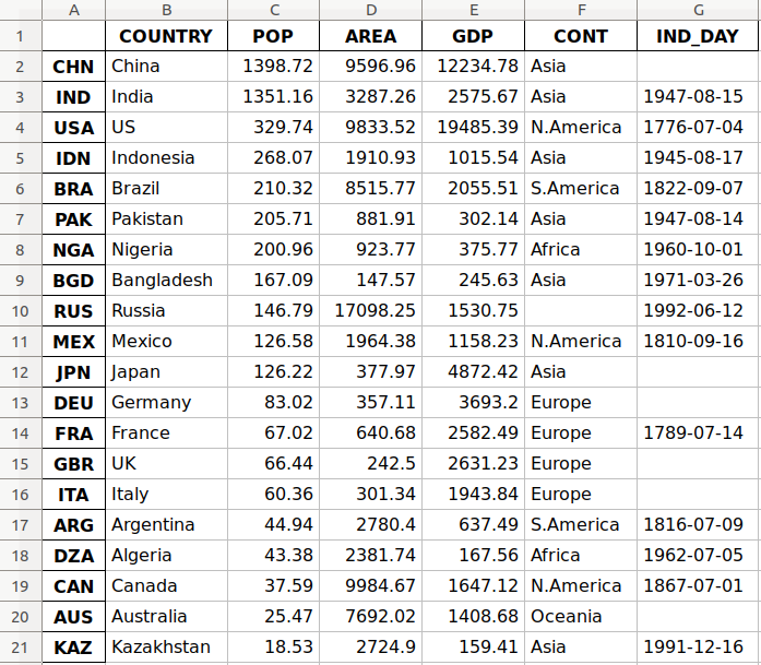
The first column of the file contains the labels of the rows, while the other columns store data.
Read an Excel File
You can load data from Excel files with read_excel():
>>>
>>> df = pd.read_excel('data.xlsx', index_col=0)
>>> df
        COUNTRY      POP      AREA       GDP       CONT     IND_DAY
CHN       China  1398.72   9596.96  12234.78       Asia         NaN
IND       India  1351.16   3287.26   2575.67       Asia  1947-08-15
USA          US   329.74   9833.52  19485.39  N.America  1776-07-04
IDN   Indonesia   268.07   1910.93   1015.54       Asia  1945-08-17
BRA      Brazil   210.32   8515.77   2055.51  S.America  1822-09-07
PAK    Pakistan   205.71    881.91    302.14       Asia  1947-08-14
NGA     Nigeria   200.96    923.77    375.77     Africa  1960-10-01
BGD  Bangladesh   167.09    147.57    245.63       Asia  1971-03-26
RUS      Russia   146.79  17098.25   1530.75        NaN  1992-06-12
MEX      Mexico   126.58   1964.38   1158.23  N.America  1810-09-16
JPN       Japan   126.22    377.97   4872.42       Asia         NaN
DEU     Germany    83.02    357.11   3693.20     Europe         NaN
FRA      France    67.02    640.68   2582.49     Europe  1789-07-14
GBR          UK    66.44    242.50   2631.23     Europe         NaN
ITA       Italy    60.36    301.34   1943.84     Europe         NaN
ARG   Argentina    44.94   2780.40    637.49  S.America  1816-07-09
DZA     Algeria    43.38   2381.74    167.56     Africa  1962-07-05
CAN      Canada    37.59   9984.67   1647.12  N.America  1867-07-01
AUS   Australia    25.47   7692.02   1408.68    Oceania         NaN
KAZ  Kazakhstan    18.53   2724.90    159.41       Asia  1991-12-16
read_excel() returns a new DataFrame that contains the values from data.xlsx. You can also use read_excel() with OpenDocument spreadsheets, or .ods files.
You’ll learn more about working with Excel files later on in this tutorial. You can also check out Using pandas to Read Large Excel Files in Python.
Understanding the pandas IO API
pandas IO Tools is the API that allows you to save the contents of Series and DataFrame objects to the clipboard, objects, or files of various types. It also enables loading data from the clipboard, objects, or files.
Write Files
Series and DataFrame objects have methods that enable writing data and labels to the clipboard or files. They’re named with the pattern .to_<file-type>(), where <file-type> is the type of the target file.
You’ve learned about .to_csv() and .to_excel(), but there are others, including:
.to_json().to_html().to_sql().to_pickle()
There are still more file types that you can write to, so this list is not exhaustive.
These methods have parameters specifying the target file path where you saved the data and labels. This is mandatory in some cases and optional in others. If this option is available and you choose to omit it, then the methods return the objects (like strings or iterables) with the contents of DataFrame instances.
The optional parameter compression decides how to compress the file with the data and labels. You’ll learn more about it later on. There are a few other parameters, but they’re mostly specific to one or several methods. You won’t go into them in detail here.
Read Files
pandas functions for reading the contents of files are named using the pattern .read_<file-type>(), where <file-type> indicates the type of the file to read. You’ve already seen the pandas read_csv() and read_excel() functions. Here are a few others:
read_json()read_html()read_sql()read_pickle()
These functions have a parameter that specifies the target file path. It can be any valid string that represents the path, either on a local machine or in a URL. Other objects are also acceptable depending on the file type.
The optional parameter compression determines the type of decompression to use for the compressed files. You’ll learn about it later on in this tutorial. There are other parameters, but they’re specific to one or several functions. You won’t go into them in detail here.
Working With Different File Types
The pandas library offers a wide range of possibilities for saving your data to files and loading data from files. In this section, you’ll learn more about working with CSV and Excel files. You’ll also see how to use other types of files, like JSON, web pages, databases, and Python pickle files.
CSV Files
You’ve already learned how to read and write CSV files. Now let’s dig a little deeper into the details. When you use .to_csv() to save your DataFrame, you can provide an argument for the parameter path_or_buf to specify the path, name, and extension of the target file.
path_or_buf is the first argument .to_csv() will get. It can be any string that represents a valid file path that includes the file name and its extension. You’ve seen this in a previous example. However, if you omit path_or_buf, then .to_csv() won’t create any files. Instead, it’ll return the corresponding string:
>>>
>>> df = pd.DataFrame(data=data).T
>>> s = df.to_csv()
>>> print(s)
,COUNTRY,POP,AREA,GDP,CONT,IND_DAY
CHN,China,1398.72,9596.96,12234.78,Asia,
IND,India,1351.16,3287.26,2575.67,Asia,1947-08-15
USA,US,329.74,9833.52,19485.39,N.America,1776-07-04
IDN,Indonesia,268.07,1910.93,1015.54,Asia,1945-08-17
BRA,Brazil,210.32,8515.77,2055.51,S.America,1822-09-07
PAK,Pakistan,205.71,881.91,302.14,Asia,1947-08-14
NGA,Nigeria,200.96,923.77,375.77,Africa,1960-10-01
BGD,Bangladesh,167.09,147.57,245.63,Asia,1971-03-26
RUS,Russia,146.79,17098.25,1530.75,,1992-06-12
MEX,Mexico,126.58,1964.38,1158.23,N.America,1810-09-16
JPN,Japan,126.22,377.97,4872.42,Asia,
DEU,Germany,83.02,357.11,3693.2,Europe,
FRA,France,67.02,640.68,2582.49,Europe,1789-07-14
GBR,UK,66.44,242.5,2631.23,Europe,
ITA,Italy,60.36,301.34,1943.84,Europe,
ARG,Argentina,44.94,2780.4,637.49,S.America,1816-07-09
DZA,Algeria,43.38,2381.74,167.56,Africa,1962-07-05
CAN,Canada,37.59,9984.67,1647.12,N.America,1867-07-01
AUS,Australia,25.47,7692.02,1408.68,Oceania,
KAZ,Kazakhstan,18.53,2724.9,159.41,Asia,1991-12-16
Now you have the string s instead of a CSV file. You also have some missing values in your DataFrame object. For example, the continent for Russia and the independence days for several countries (China, Japan, and so on) are not available. In data science and machine learning, you must handle missing values carefully. pandas excels here! By default, pandas uses the NaN value to replace the missing values.
The continent that corresponds to Russia in df is nan:
>>>
>>> df.loc['RUS', 'CONT']
nan
This example uses .loc[] to get data with the specified row and column names.
When you save your DataFrame to a CSV file, empty strings ('') will represent the missing data. You can see this both in your file data.csv and in the string s. If you want to change this behavior, then use the optional parameter na_rep:
>>>
>>> df.to_csv('new-data.csv', na_rep='(missing)')
This code produces the file new-data.csv where the missing values are no longer empty strings. You can expand the code block below to see how this file should look:
,COUNTRY,POP,AREA,GDP,CONT,IND_DAY
CHN,China,1398.72,9596.96,12234.78,Asia,(missing)
IND,India,1351.16,3287.26,2575.67,Asia,1947-08-15
USA,US,329.74,9833.52,19485.39,N.America,1776-07-04
IDN,Indonesia,268.07,1910.93,1015.54,Asia,1945-08-17
BRA,Brazil,210.32,8515.77,2055.51,S.America,1822-09-07
PAK,Pakistan,205.71,881.91,302.14,Asia,1947-08-14
NGA,Nigeria,200.96,923.77,375.77,Africa,1960-10-01
BGD,Bangladesh,167.09,147.57,245.63,Asia,1971-03-26
RUS,Russia,146.79,17098.25,1530.75,(missing),1992-06-12
MEX,Mexico,126.58,1964.38,1158.23,N.America,1810-09-16
JPN,Japan,126.22,377.97,4872.42,Asia,(missing)
DEU,Germany,83.02,357.11,3693.2,Europe,(missing)
FRA,France,67.02,640.68,2582.49,Europe,1789-07-14
GBR,UK,66.44,242.5,2631.23,Europe,(missing)
ITA,Italy,60.36,301.34,1943.84,Europe,(missing)
ARG,Argentina,44.94,2780.4,637.49,S.America,1816-07-09
DZA,Algeria,43.38,2381.74,167.56,Africa,1962-07-05
CAN,Canada,37.59,9984.67,1647.12,N.America,1867-07-01
AUS,Australia,25.47,7692.02,1408.68,Oceania,(missing)
KAZ,Kazakhstan,18.53,2724.9,159.41,Asia,1991-12-16
Now, the string '(missing)' in the file corresponds to the nan values from df.
When pandas reads files, it considers the empty string ('') and a few others as missing values by default:
'nan''-nan''NA''N/A''NaN''null'
If you don’t want this behavior, then you can pass keep_default_na=False to the pandas read_csv() function. To specify other labels for missing values, use the parameter na_values:
>>>
>>> pd.read_csv('new-data.csv', index_col=0, na_values='(missing)')
        COUNTRY      POP      AREA       GDP       CONT     IND_DAY
CHN       China  1398.72   9596.96  12234.78       Asia         NaN
IND       India  1351.16   3287.26   2575.67       Asia  1947-08-15
USA          US   329.74   9833.52  19485.39  N.America  1776-07-04
IDN   Indonesia   268.07   1910.93   1015.54       Asia  1945-08-17
BRA      Brazil   210.32   8515.77   2055.51  S.America  1822-09-07
PAK    Pakistan   205.71    881.91    302.14       Asia  1947-08-14
NGA     Nigeria   200.96    923.77    375.77     Africa  1960-10-01
BGD  Bangladesh   167.09    147.57    245.63       Asia  1971-03-26
RUS      Russia   146.79  17098.25   1530.75        NaN  1992-06-12
MEX      Mexico   126.58   1964.38   1158.23  N.America  1810-09-16
JPN       Japan   126.22    377.97   4872.42       Asia         NaN
DEU     Germany    83.02    357.11   3693.20     Europe         NaN
FRA      France    67.02    640.68   2582.49     Europe  1789-07-14
GBR          UK    66.44    242.50   2631.23     Europe         NaN
ITA       Italy    60.36    301.34   1943.84     Europe         NaN
ARG   Argentina    44.94   2780.40    637.49  S.America  1816-07-09
DZA     Algeria    43.38   2381.74    167.56     Africa  1962-07-05
CAN      Canada    37.59   9984.67   1647.12  N.America  1867-07-01
AUS   Australia    25.47   7692.02   1408.68    Oceania         NaN
KAZ  Kazakhstan    18.53   2724.90    159.41       Asia  1991-12-16
Here, you’ve marked the string '(missing)' as a new missing data label, and pandas replaced it with nan when it read the file.
When you load data from a file, pandas assigns the data types to the values of each column by default. You can check these types with .dtypes:
>>>
>>> df = pd.read_csv('data.csv', index_col=0)
>>> df.dtypes
COUNTRY     object
POP        float64
AREA       float64
GDP        float64
CONT        object
IND_DAY     object
dtype: object
The columns with strings and dates ('COUNTRY', 'CONT', and 'IND_DAY') have the data type object. Meanwhile, the numeric columns contain 64-bit floating-point numbers (float64).
You can use the parameter dtype to specify the desired data types and parse_dates to force use of datetimes:
>>>
>>> dtypes = {'POP': 'float32', 'AREA': 'float32', 'GDP': 'float32'}
>>> df = pd.read_csv('data.csv', index_col=0, dtype=dtypes,
...                  parse_dates=['IND_DAY'])
>>> df.dtypes
COUNTRY            object
POP               float32
AREA              float32
GDP               float32
CONT               object
IND_DAY    datetime64[ns]
dtype: object
>>> df['IND_DAY']
CHN          NaT
IND   1947-08-15
USA   1776-07-04
IDN   1945-08-17
BRA   1822-09-07
PAK   1947-08-14
NGA   1960-10-01
BGD   1971-03-26
RUS   1992-06-12
MEX   1810-09-16
JPN          NaT
DEU          NaT
FRA   1789-07-14
GBR          NaT
ITA          NaT
ARG   1816-07-09
DZA   1962-07-05
CAN   1867-07-01
AUS          NaT
KAZ   1991-12-16
Name: IND_DAY, dtype: datetime64[ns]
Now, you have 32-bit floating-point numbers (float32) as specified with dtype. These differ slightly from the original 64-bit numbers because of smaller precision. The values in the last column are considered as dates and have the data type datetime64. That’s why the NaN values in this column are replaced with NaT.
Now that you have real dates, you can save them in the format you like:
>>>
>>> df = pd.read_csv('data.csv', index_col=0, parse_dates=['IND_DAY'])
>>> df.to_csv('formatted-data.csv', date_format='%B %d, %Y')
Here, you’ve specified the parameter date_format to be '%B %d, %Y'. You can expand the code block below to see the resulting file:
,COUNTRY,POP,AREA,GDP,CONT,IND_DAY
CHN,China,1398.72,9596.96,12234.78,Asia,
IND,India,1351.16,3287.26,2575.67,Asia,"August 15, 1947"
USA,US,329.74,9833.52,19485.39,N.America,"July 04, 1776"
IDN,Indonesia,268.07,1910.93,1015.54,Asia,"August 17, 1945"
BRA,Brazil,210.32,8515.77,2055.51,S.America,"September 07, 1822"
PAK,Pakistan,205.71,881.91,302.14,Asia,"August 14, 1947"
NGA,Nigeria,200.96,923.77,375.77,Africa,"October 01, 1960"
BGD,Bangladesh,167.09,147.57,245.63,Asia,"March 26, 1971"
RUS,Russia,146.79,17098.25,1530.75,,"June 12, 1992"
MEX,Mexico,126.58,1964.38,1158.23,N.America,"September 16, 1810"
JPN,Japan,126.22,377.97,4872.42,Asia,
DEU,Germany,83.02,357.11,3693.2,Europe,
FRA,France,67.02,640.68,2582.49,Europe,"July 14, 1789"
GBR,UK,66.44,242.5,2631.23,Europe,
ITA,Italy,60.36,301.34,1943.84,Europe,
ARG,Argentina,44.94,2780.4,637.49,S.America,"July 09, 1816"
DZA,Algeria,43.38,2381.74,167.56,Africa,"July 05, 1962"
CAN,Canada,37.59,9984.67,1647.12,N.America,"July 01, 1867"
AUS,Australia,25.47,7692.02,1408.68,Oceania,
KAZ,Kazakhstan,18.53,2724.9,159.41,Asia,"December 16, 1991"
The format of the dates is different now. The format '%B %d, %Y' means the date will first display the full name of the month, then the day followed by a comma, and finally the full year.
There are several other optional parameters that you can use with .to_csv():
sepdenotes a values separator.decimalindicates a decimal separator.encodingsets the file encoding.headerspecifies whether you want to write column labels in the file.
Here’s how you would pass arguments for sep and header:
>>>
>>> s = df.to_csv(sep=';', header=False)
>>> print(s)
CHN;China;1398.72;9596.96;12234.78;Asia;
IND;India;1351.16;3287.26;2575.67;Asia;1947-08-15
USA;US;329.74;9833.52;19485.39;N.America;1776-07-04
IDN;Indonesia;268.07;1910.93;1015.54;Asia;1945-08-17
BRA;Brazil;210.32;8515.77;2055.51;S.America;1822-09-07
PAK;Pakistan;205.71;881.91;302.14;Asia;1947-08-14
NGA;Nigeria;200.96;923.77;375.77;Africa;1960-10-01
BGD;Bangladesh;167.09;147.57;245.63;Asia;1971-03-26
RUS;Russia;146.79;17098.25;1530.75;;1992-06-12
MEX;Mexico;126.58;1964.38;1158.23;N.America;1810-09-16
JPN;Japan;126.22;377.97;4872.42;Asia;
DEU;Germany;83.02;357.11;3693.2;Europe;
FRA;France;67.02;640.68;2582.49;Europe;1789-07-14
GBR;UK;66.44;242.5;2631.23;Europe;
ITA;Italy;60.36;301.34;1943.84;Europe;
ARG;Argentina;44.94;2780.4;637.49;S.America;1816-07-09
DZA;Algeria;43.38;2381.74;167.56;Africa;1962-07-05
CAN;Canada;37.59;9984.67;1647.12;N.America;1867-07-01
AUS;Australia;25.47;7692.02;1408.68;Oceania;
KAZ;Kazakhstan;18.53;2724.9;159.41;Asia;1991-12-16
The data is separated with a semicolon (';') because you’ve specified sep=';'. Also, since you passed header=False, you see your data without the header row of column names.
The pandas read_csv() function has many additional options for managing missing data, working with dates and times, quoting, encoding, handling errors, and more. For instance, if you have a file with one data column and want to get a Series object instead of a DataFrame, then you can pass squeeze=True to read_csv(). You’ll learn later on about data compression and decompression, as well as how to skip rows and columns.
JSON Files
JSON stands for JavaScript object notation. JSON files are plaintext files used for data interchange, and humans can read them easily. They follow the ISO/IEC 21778:2017 and ECMA-404 standards and use the .json extension. Python and pandas work well with JSON files, as Python’s json library offers built-in support for them.
You can save the data from your DataFrame to a JSON file with .to_json(). Start by creating a DataFrame object again. Use the dictionary data that holds the data about countries and then apply .to_json():
>>>
>>> df = pd.DataFrame(data=data).T
>>> df.to_json('data-columns.json')
This code produces the file data-columns.json. You can expand the code block below to see how this file should look:
{"COUNTRY":{"CHN":"China","IND":"India","USA":"US","IDN":"Indonesia","BRA":"Brazil","PAK":"Pakistan","NGA":"Nigeria","BGD":"Bangladesh","RUS":"Russia","MEX":"Mexico","JPN":"Japan","DEU":"Germany","FRA":"France","GBR":"UK","ITA":"Italy","ARG":"Argentina","DZA":"Algeria","CAN":"Canada","AUS":"Australia","KAZ":"Kazakhstan"},"POP":{"CHN":1398.72,"IND":1351.16,"USA":329.74,"IDN":268.07,"BRA":210.32,"PAK":205.71,"NGA":200.96,"BGD":167.09,"RUS":146.79,"MEX":126.58,"JPN":126.22,"DEU":83.02,"FRA":67.02,"GBR":66.44,"ITA":60.36,"ARG":44.94,"DZA":43.38,"CAN":37.59,"AUS":25.47,"KAZ":18.53},"AREA":{"CHN":9596.96,"IND":3287.26,"USA":9833.52,"IDN":1910.93,"BRA":8515.77,"PAK":881.91,"NGA":923.77,"BGD":147.57,"RUS":17098.25,"MEX":1964.38,"JPN":377.97,"DEU":357.11,"FRA":640.68,"GBR":242.5,"ITA":301.34,"ARG":2780.4,"DZA":2381.74,"CAN":9984.67,"AUS":7692.02,"KAZ":2724.9},"GDP":{"CHN":12234.78,"IND":2575.67,"USA":19485.39,"IDN":1015.54,"BRA":2055.51,"PAK":302.14,"NGA":375.77,"BGD":245.63,"RUS":1530.75,"MEX":1158.23,"JPN":4872.42,"DEU":3693.2,"FRA":2582.49,"GBR":2631.23,"ITA":1943.84,"ARG":637.49,"DZA":167.56,"CAN":1647.12,"AUS":1408.68,"KAZ":159.41},"CONT":{"CHN":"Asia","IND":"Asia","USA":"N.America","IDN":"Asia","BRA":"S.America","PAK":"Asia","NGA":"Africa","BGD":"Asia","RUS":null,"MEX":"N.America","JPN":"Asia","DEU":"Europe","FRA":"Europe","GBR":"Europe","ITA":"Europe","ARG":"S.America","DZA":"Africa","CAN":"N.America","AUS":"Oceania","KAZ":"Asia"},"IND_DAY":{"CHN":null,"IND":"1947-08-15","USA":"1776-07-04","IDN":"1945-08-17","BRA":"1822-09-07","PAK":"1947-08-14","NGA":"1960-10-01","BGD":"1971-03-26","RUS":"1992-06-12","MEX":"1810-09-16","JPN":null,"DEU":null,"FRA":"1789-07-14","GBR":null,"ITA":null,"ARG":"1816-07-09","DZA":"1962-07-05","CAN":"1867-07-01","AUS":null,"KAZ":"1991-12-16"}}
data-columns.json has one large dictionary with the column labels as keys and the corresponding inner dictionaries as values.
You can get a different file structure if you pass an argument for the optional parameter orient:
>>>
>>> df.to_json('data-index.json', orient='index')
The orient parameter defaults to 'columns'. Here, you’ve set it to index.
You should get a new file data-index.json. You can expand the code block below to see the changes:
{"CHN":{"COUNTRY":"China","POP":1398.72,"AREA":9596.96,"GDP":12234.78,"CONT":"Asia","IND_DAY":null},"IND":{"COUNTRY":"India","POP":1351.16,"AREA":3287.26,"GDP":2575.67,"CONT":"Asia","IND_DAY":"1947-08-15"},"USA":{"COUNTRY":"US","POP":329.74,"AREA":9833.52,"GDP":19485.39,"CONT":"N.America","IND_DAY":"1776-07-04"},"IDN":{"COUNTRY":"Indonesia","POP":268.07,"AREA":1910.93,"GDP":1015.54,"CONT":"Asia","IND_DAY":"1945-08-17"},"BRA":{"COUNTRY":"Brazil","POP":210.32,"AREA":8515.77,"GDP":2055.51,"CONT":"S.America","IND_DAY":"1822-09-07"},"PAK":{"COUNTRY":"Pakistan","POP":205.71,"AREA":881.91,"GDP":302.14,"CONT":"Asia","IND_DAY":"1947-08-14"},"NGA":{"COUNTRY":"Nigeria","POP":200.96,"AREA":923.77,"GDP":375.77,"CONT":"Africa","IND_DAY":"1960-10-01"},"BGD":{"COUNTRY":"Bangladesh","POP":167.09,"AREA":147.57,"GDP":245.63,"CONT":"Asia","IND_DAY":"1971-03-26"},"RUS":{"COUNTRY":"Russia","POP":146.79,"AREA":17098.25,"GDP":1530.75,"CONT":null,"IND_DAY":"1992-06-12"},"MEX":{"COUNTRY":"Mexico","POP":126.58,"AREA":1964.38,"GDP":1158.23,"CONT":"N.America","IND_DAY":"1810-09-16"},"JPN":{"COUNTRY":"Japan","POP":126.22,"AREA":377.97,"GDP":4872.42,"CONT":"Asia","IND_DAY":null},"DEU":{"COUNTRY":"Germany","POP":83.02,"AREA":357.11,"GDP":3693.2,"CONT":"Europe","IND_DAY":null},"FRA":{"COUNTRY":"France","POP":67.02,"AREA":640.68,"GDP":2582.49,"CONT":"Europe","IND_DAY":"1789-07-14"},"GBR":{"COUNTRY":"UK","POP":66.44,"AREA":242.5,"GDP":2631.23,"CONT":"Europe","IND_DAY":null},"ITA":{"COUNTRY":"Italy","POP":60.36,"AREA":301.34,"GDP":1943.84,"CONT":"Europe","IND_DAY":null},"ARG":{"COUNTRY":"Argentina","POP":44.94,"AREA":2780.4,"GDP":637.49,"CONT":"S.America","IND_DAY":"1816-07-09"},"DZA":{"COUNTRY":"Algeria","POP":43.38,"AREA":2381.74,"GDP":167.56,"CONT":"Africa","IND_DAY":"1962-07-05"},"CAN":{"COUNTRY":"Canada","POP":37.59,"AREA":9984.67,"GDP":1647.12,"CONT":"N.America","IND_DAY":"1867-07-01"},"AUS":{"COUNTRY":"Australia","POP":25.47,"AREA":7692.02,"GDP":1408.68,"CONT":"Oceania","IND_DAY":null},"KAZ":{"COUNTRY":"Kazakhstan","POP":18.53,"AREA":2724.9,"GDP":159.41,"CONT":"Asia","IND_DAY":"1991-12-16"}}
data-index.json also has one large dictionary, but this time the row labels are the keys, and the inner dictionaries are the values.
There are few more options for orient. One of them is 'records':
>>>
>>> df.to_json('data-records.json', orient='records')
This code should yield the file data-records.json. You can expand the code block below to see the content:
[{"COUNTRY":"China","POP":1398.72,"AREA":9596.96,"GDP":12234.78,"CONT":"Asia","IND_DAY":null},{"COUNTRY":"India","POP":1351.16,"AREA":3287.26,"GDP":2575.67,"CONT":"Asia","IND_DAY":"1947-08-15"},{"COUNTRY":"US","POP":329.74,"AREA":9833.52,"GDP":19485.39,"CONT":"N.America","IND_DAY":"1776-07-04"},{"COUNTRY":"Indonesia","POP":268.07,"AREA":1910.93,"GDP":1015.54,"CONT":"Asia","IND_DAY":"1945-08-17"},{"COUNTRY":"Brazil","POP":210.32,"AREA":8515.77,"GDP":2055.51,"CONT":"S.America","IND_DAY":"1822-09-07"},{"COUNTRY":"Pakistan","POP":205.71,"AREA":881.91,"GDP":302.14,"CONT":"Asia","IND_DAY":"1947-08-14"},{"COUNTRY":"Nigeria","POP":200.96,"AREA":923.77,"GDP":375.77,"CONT":"Africa","IND_DAY":"1960-10-01"},{"COUNTRY":"Bangladesh","POP":167.09,"AREA":147.57,"GDP":245.63,"CONT":"Asia","IND_DAY":"1971-03-26"},{"COUNTRY":"Russia","POP":146.79,"AREA":17098.25,"GDP":1530.75,"CONT":null,"IND_DAY":"1992-06-12"},{"COUNTRY":"Mexico","POP":126.58,"AREA":1964.38,"GDP":1158.23,"CONT":"N.America","IND_DAY":"1810-09-16"},{"COUNTRY":"Japan","POP":126.22,"AREA":377.97,"GDP":4872.42,"CONT":"Asia","IND_DAY":null},{"COUNTRY":"Germany","POP":83.02,"AREA":357.11,"GDP":3693.2,"CONT":"Europe","IND_DAY":null},{"COUNTRY":"France","POP":67.02,"AREA":640.68,"GDP":2582.49,"CONT":"Europe","IND_DAY":"1789-07-14"},{"COUNTRY":"UK","POP":66.44,"AREA":242.5,"GDP":2631.23,"CONT":"Europe","IND_DAY":null},{"COUNTRY":"Italy","POP":60.36,"AREA":301.34,"GDP":1943.84,"CONT":"Europe","IND_DAY":null},{"COUNTRY":"Argentina","POP":44.94,"AREA":2780.4,"GDP":637.49,"CONT":"S.America","IND_DAY":"1816-07-09"},{"COUNTRY":"Algeria","POP":43.38,"AREA":2381.74,"GDP":167.56,"CONT":"Africa","IND_DAY":"1962-07-05"},{"COUNTRY":"Canada","POP":37.59,"AREA":9984.67,"GDP":1647.12,"CONT":"N.America","IND_DAY":"1867-07-01"},{"COUNTRY":"Australia","POP":25.47,"AREA":7692.02,"GDP":1408.68,"CONT":"Oceania","IND_DAY":null},{"COUNTRY":"Kazakhstan","POP":18.53,"AREA":2724.9,"GDP":159.41,"CONT":"Asia","IND_DAY":"1991-12-16"}]
data-records.json holds a list with one dictionary for each row. The row labels are not written.
You can get another interesting file structure with orient='split':
>>>
>>> df.to_json('data-split.json', orient='split')
The resulting file is data-split.json. You can expand the code block below to see how this file should look:
{"columns":["COUNTRY","POP","AREA","GDP","CONT","IND_DAY"],"index":["CHN","IND","USA","IDN","BRA","PAK","NGA","BGD","RUS","MEX","JPN","DEU","FRA","GBR","ITA","ARG","DZA","CAN","AUS","KAZ"],"data":[["China",1398.72,9596.96,12234.78,"Asia",null],["India",1351.16,3287.26,2575.67,"Asia","1947-08-15"],["US",329.74,9833.52,19485.39,"N.America","1776-07-04"],["Indonesia",268.07,1910.93,1015.54,"Asia","1945-08-17"],["Brazil",210.32,8515.77,2055.51,"S.America","1822-09-07"],["Pakistan",205.71,881.91,302.14,"Asia","1947-08-14"],["Nigeria",200.96,923.77,375.77,"Africa","1960-10-01"],["Bangladesh",167.09,147.57,245.63,"Asia","1971-03-26"],["Russia",146.79,17098.25,1530.75,null,"1992-06-12"],["Mexico",126.58,1964.38,1158.23,"N.America","1810-09-16"],["Japan",126.22,377.97,4872.42,"Asia",null],["Germany",83.02,357.11,3693.2,"Europe",null],["France",67.02,640.68,2582.49,"Europe","1789-07-14"],["UK",66.44,242.5,2631.23,"Europe",null],["Italy",60.36,301.34,1943.84,"Europe",null],["Argentina",44.94,2780.4,637.49,"S.America","1816-07-09"],["Algeria",43.38,2381.74,167.56,"Africa","1962-07-05"],["Canada",37.59,9984.67,1647.12,"N.America","1867-07-01"],["Australia",25.47,7692.02,1408.68,"Oceania",null],["Kazakhstan",18.53,2724.9,159.41,"Asia","1991-12-16"]]}
data-split.json contains one dictionary that holds the following lists:
- The names of the columns
- The labels of the rows
- The inner lists (two-dimensional sequence) that hold data values
If you don’t provide the value for the optional parameter path_or_buf that defines the file path, then .to_json() will return a JSON string instead of writing the results to a file. This behavior is consistent with .to_csv().
There are other optional parameters you can use. For instance, you can set index=False to forgo saving row labels. You can manipulate precision with double_precision, and dates with date_format and date_unit. These last two parameters are particularly important when you have time series among your data:
>>>
>>> df = pd.DataFrame(data=data).T
>>> df['IND_DAY'] = pd.to_datetime(df['IND_DAY'])
>>> df.dtypes
COUNTRY            object
POP                object
AREA               object
GDP                object
CONT               object
IND_DAY    datetime64[ns]
dtype: object

>>> df.to_json('data-time.json')
In this example, you’ve created the DataFrame from the dictionary data and used to_datetime() to convert the values in the last column to datetime64. You can expand the code block below to see the resulting file:
{"COUNTRY":{"CHN":"China","IND":"India","USA":"US","IDN":"Indonesia","BRA":"Brazil","PAK":"Pakistan","NGA":"Nigeria","BGD":"Bangladesh","RUS":"Russia","MEX":"Mexico","JPN":"Japan","DEU":"Germany","FRA":"France","GBR":"UK","ITA":"Italy","ARG":"Argentina","DZA":"Algeria","CAN":"Canada","AUS":"Australia","KAZ":"Kazakhstan"},"POP":{"CHN":1398.72,"IND":1351.16,"USA":329.74,"IDN":268.07,"BRA":210.32,"PAK":205.71,"NGA":200.96,"BGD":167.09,"RUS":146.79,"MEX":126.58,"JPN":126.22,"DEU":83.02,"FRA":67.02,"GBR":66.44,"ITA":60.36,"ARG":44.94,"DZA":43.38,"CAN":37.59,"AUS":25.47,"KAZ":18.53},"AREA":{"CHN":9596.96,"IND":3287.26,"USA":9833.52,"IDN":1910.93,"BRA":8515.77,"PAK":881.91,"NGA":923.77,"BGD":147.57,"RUS":17098.25,"MEX":1964.38,"JPN":377.97,"DEU":357.11,"FRA":640.68,"GBR":242.5,"ITA":301.34,"ARG":2780.4,"DZA":2381.74,"CAN":9984.67,"AUS":7692.02,"KAZ":2724.9},"GDP":{"CHN":12234.78,"IND":2575.67,"USA":19485.39,"IDN":1015.54,"BRA":2055.51,"PAK":302.14,"NGA":375.77,"BGD":245.63,"RUS":1530.75,"MEX":1158.23,"JPN":4872.42,"DEU":3693.2,"FRA":2582.49,"GBR":2631.23,"ITA":1943.84,"ARG":637.49,"DZA":167.56,"CAN":1647.12,"AUS":1408.68,"KAZ":159.41},"CONT":{"CHN":"Asia","IND":"Asia","USA":"N.America","IDN":"Asia","BRA":"S.America","PAK":"Asia","NGA":"Africa","BGD":"Asia","RUS":null,"MEX":"N.America","JPN":"Asia","DEU":"Europe","FRA":"Europe","GBR":"Europe","ITA":"Europe","ARG":"S.America","DZA":"Africa","CAN":"N.America","AUS":"Oceania","KAZ":"Asia"},"IND_DAY":{"CHN":null,"IND":-706320000000,"USA":-6106060800000,"IDN":-769219200000,"BRA":-4648924800000,"PAK":-706406400000,"NGA":-291945600000,"BGD":38793600000,"RUS":708307200000,"MEX":-5026838400000,"JPN":null,"DEU":null,"FRA":-5694969600000,"GBR":null,"ITA":null,"ARG":-4843411200000,"DZA":-236476800000,"CAN":-3234729600000,"AUS":null,"KAZ":692841600000}}
In this file, you have large integers instead of dates for the independence days. That’s because the default value of the optional parameter date_format is 'epoch' whenever orient isn’t 'table'. This default behavior expresses dates as an epoch in milliseconds relative to midnight on January 1, 1970.
However, if you pass date_format='iso', then you’ll get the dates in the ISO 8601 format. In addition, date_unit decides the units of time:
>>>
>>> df = pd.DataFrame(data=data).T
>>> df['IND_DAY'] = pd.to_datetime(df['IND_DAY'])
>>> df.to_json('new-data-time.json', date_format='iso', date_unit='s')
This code produces the following JSON file:
{"COUNTRY":{"CHN":"China","IND":"India","USA":"US","IDN":"Indonesia","BRA":"Brazil","PAK":"Pakistan","NGA":"Nigeria","BGD":"Bangladesh","RUS":"Russia","MEX":"Mexico","JPN":"Japan","DEU":"Germany","FRA":"France","GBR":"UK","ITA":"Italy","ARG":"Argentina","DZA":"Algeria","CAN":"Canada","AUS":"Australia","KAZ":"Kazakhstan"},"POP":{"CHN":1398.72,"IND":1351.16,"USA":329.74,"IDN":268.07,"BRA":210.32,"PAK":205.71,"NGA":200.96,"BGD":167.09,"RUS":146.79,"MEX":126.58,"JPN":126.22,"DEU":83.02,"FRA":67.02,"GBR":66.44,"ITA":60.36,"ARG":44.94,"DZA":43.38,"CAN":37.59,"AUS":25.47,"KAZ":18.53},"AREA":{"CHN":9596.96,"IND":3287.26,"USA":9833.52,"IDN":1910.93,"BRA":8515.77,"PAK":881.91,"NGA":923.77,"BGD":147.57,"RUS":17098.25,"MEX":1964.38,"JPN":377.97,"DEU":357.11,"FRA":640.68,"GBR":242.5,"ITA":301.34,"ARG":2780.4,"DZA":2381.74,"CAN":9984.67,"AUS":7692.02,"KAZ":2724.9},"GDP":{"CHN":12234.78,"IND":2575.67,"USA":19485.39,"IDN":1015.54,"BRA":2055.51,"PAK":302.14,"NGA":375.77,"BGD":245.63,"RUS":1530.75,"MEX":1158.23,"JPN":4872.42,"DEU":3693.2,"FRA":2582.49,"GBR":2631.23,"ITA":1943.84,"ARG":637.49,"DZA":167.56,"CAN":1647.12,"AUS":1408.68,"KAZ":159.41},"CONT":{"CHN":"Asia","IND":"Asia","USA":"N.America","IDN":"Asia","BRA":"S.America","PAK":"Asia","NGA":"Africa","BGD":"Asia","RUS":null,"MEX":"N.America","JPN":"Asia","DEU":"Europe","FRA":"Europe","GBR":"Europe","ITA":"Europe","ARG":"S.America","DZA":"Africa","CAN":"N.America","AUS":"Oceania","KAZ":"Asia"},"IND_DAY":{"CHN":null,"IND":"1947-08-15T00:00:00Z","USA":"1776-07-04T00:00:00Z","IDN":"1945-08-17T00:00:00Z","BRA":"1822-09-07T00:00:00Z","PAK":"1947-08-14T00:00:00Z","NGA":"1960-10-01T00:00:00Z","BGD":"1971-03-26T00:00:00Z","RUS":"1992-06-12T00:00:00Z","MEX":"1810-09-16T00:00:00Z","JPN":null,"DEU":null,"FRA":"1789-07-14T00:00:00Z","GBR":null,"ITA":null,"ARG":"1816-07-09T00:00:00Z","DZA":"1962-07-05T00:00:00Z","CAN":"1867-07-01T00:00:00Z","AUS":null,"KAZ":"1991-12-16T00:00:00Z"}}
The dates in the resulting file are in the ISO 8601 format.
You can load the data from a JSON file with read_json():
>>>
>>> df = pd.read_json('data-index.json', orient='index',
...                   convert_dates=['IND_DAY'])
The parameter convert_dates has a similar purpose as parse_dates when you use it to read CSV files. The optional parameter orient is very important because it specifies how pandas understands the structure of the file.
There are other optional parameters you can use as well:
- Set the encoding with
encoding. - Manipulate dates with
convert_datesandkeep_default_dates. - Impact precision with
dtypeandprecise_float. - Decode numeric data directly to NumPy arrays with
numpy=True.
Note that you might lose the order of rows and columns when using the JSON format to store your data.
HTML Files
An HTML is a plaintext file that uses hypertext markup language to help browsers render web pages. The extensions for HTML files are .html and .htm. You’ll need to install an HTML parser library like lxml or html5lib to be able to work with HTML files:
$pip install lxml html5lib
You can also use Conda to install the same packages:
$ conda install lxml html5lib
Once you have these libraries, you can save the contents of your DataFrame as an HTML file with .to_html():
>>>
df = pd.DataFrame(data=data).T
df.to_html('data.html')
This code generates a file data.html. You can expand the code block below to see how this file should look:
<table border="1" class="dataframe">
  <thead>
    <tr style="text-align: right;">
      <th></th>
      <th>COUNTRY</th>
      <th>POP</th>
      <th>AREA</th>
      <th>GDP</th>
      <th>CONT</th>
      <th>IND_DAY</th>
    </tr>
  </thead>
  <tbody>
    <tr>
      <th>CHN</th>
      <td>China</td>
      <td>1398.72</td>
      <td>9596.96</td>
      <td>12234.8</td>
      <td>Asia</td>
      <td>NaN</td>
    </tr>
    <tr>
      <th>IND</th>
      <td>India</td>
      <td>1351.16</td>
      <td>3287.26</td>
      <td>2575.67</td>
      <td>Asia</td>
      <td>1947-08-15</td>
    </tr>
    <tr>
      <th>USA</th>
      <td>US</td>
      <td>329.74</td>
      <td>9833.52</td>
      <td>19485.4</td>
      <td>N.America</td>
      <td>1776-07-04</td>
    </tr>
    <tr>
      <th>IDN</th>
      <td>Indonesia</td>
      <td>268.07</td>
      <td>1910.93</td>
      <td>1015.54</td>
      <td>Asia</td>
      <td>1945-08-17</td>
    </tr>
    <tr>
      <th>BRA</th>
      <td>Brazil</td>
      <td>210.32</td>
      <td>8515.77</td>
      <td>2055.51</td>
      <td>S.America</td>
      <td>1822-09-07</td>
    </tr>
    <tr>
      <th>PAK</th>
      <td>Pakistan</td>
      <td>205.71</td>
      <td>881.91</td>
      <td>302.14</td>
      <td>Asia</td>
      <td>1947-08-14</td>
    </tr>
    <tr>
      <th>NGA</th>
      <td>Nigeria</td>
      <td>200.96</td>
      <td>923.77</td>
      <td>375.77</td>
      <td>Africa</td>
      <td>1960-10-01</td>
    </tr>
    <tr>
      <th>BGD</th>
      <td>Bangladesh</td>
      <td>167.09</td>
      <td>147.57</td>
      <td>245.63</td>
      <td>Asia</td>
      <td>1971-03-26</td>
    </tr>
    <tr>
      <th>RUS</th>
      <td>Russia</td>
      <td>146.79</td>
      <td>17098.2</td>
      <td>1530.75</td>
      <td>NaN</td>
      <td>1992-06-12</td>
    </tr>
    <tr>
      <th>MEX</th>
      <td>Mexico</td>
      <td>126.58</td>
      <td>1964.38</td>
      <td>1158.23</td>
      <td>N.America</td>
      <td>1810-09-16</td>
    </tr>
    <tr>
      <th>JPN</th>
      <td>Japan</td>
      <td>126.22</td>
      <td>377.97</td>
      <td>4872.42</td>
      <td>Asia</td>
      <td>NaN</td>
    </tr>
    <tr>
      <th>DEU</th>
      <td>Germany</td>
      <td>83.02</td>
      <td>357.11</td>
      <td>3693.2</td>
      <td>Europe</td>
      <td>NaN</td>
    </tr>
    <tr>
      <th>FRA</th>
      <td>France</td>
      <td>67.02</td>
      <td>640.68</td>
      <td>2582.49</td>
      <td>Europe</td>
      <td>1789-07-14</td>
    </tr>
    <tr>
      <th>GBR</th>
      <td>UK</td>
      <td>66.44</td>
      <td>242.5</td>
      <td>2631.23</td>
      <td>Europe</td>
      <td>NaN</td>
    </tr>
    <tr>
      <th>ITA</th>
      <td>Italy</td>
      <td>60.36</td>
      <td>301.34</td>
      <td>1943.84</td>
      <td>Europe</td>
      <td>NaN</td>
    </tr>
    <tr>
      <th>ARG</th>
      <td>Argentina</td>
      <td>44.94</td>
      <td>2780.4</td>
      <td>637.49</td>
      <td>S.America</td>
      <td>1816-07-09</td>
    </tr>
    <tr>
      <th>DZA</th>
      <td>Algeria</td>
      <td>43.38</td>
      <td>2381.74</td>
      <td>167.56</td>
      <td>Africa</td>
      <td>1962-07-05</td>
    </tr>
    <tr>
      <th>CAN</th>
      <td>Canada</td>
      <td>37.59</td>
      <td>9984.67</td>
      <td>1647.12</td>
      <td>N.America</td>
      <td>1867-07-01</td>
    </tr>
    <tr>
      <th>AUS</th>
      <td>Australia</td>
      <td>25.47</td>
      <td>7692.02</td>
      <td>1408.68</td>
      <td>Oceania</td>
      <td>NaN</td>
    </tr>
    <tr>
      <th>KAZ</th>
      <td>Kazakhstan</td>
      <td>18.53</td>
      <td>2724.9</td>
      <td>159.41</td>
      <td>Asia</td>
      <td>1991-12-16</td>
    </tr>
  </tbody>
</table>
This file shows the DataFrame contents nicely. However, notice that you haven’t obtained an entire web page. You’ve just output the data that corresponds to df in the HTML format.
.to_html() won’t create a file if you don’t provide the optional parameter buf, which denotes the buffer to write to. If you leave this parameter out, then your code will return a string as it did with .to_csv() and .to_json().
Here are some other optional parameters:
headerdetermines whether to save the column names.indexdetermines whether to save the row labels.classesassigns cascading style sheet (CSS) classes.render_linksspecifies whether to convert URLs to HTML links.table_idassigns the CSSidto thetabletag.escapedecides whether to convert the characters<,>, and&to HTML-safe strings.
You use parameters like these to specify different aspects of the resulting files or strings.
You can create a DataFrame object from a suitable HTML file using read_html(), which will return a DataFrame instance or a list of them:
>>>
>>> df = pd.read_html('data.html', index_col=0, parse_dates=['IND_DAY'])
This is very similar to what you did when reading CSV files. You also have parameters that help you work with dates, missing values, precision, encoding, HTML parsers, and more.
Excel Files
You’ve already learned how to read and write Excel files with pandas. However, there are a few more options worth considering. For one, when you use .to_excel(), you can specify the name of the target worksheet with the optional parameter sheet_name:
>>>
>>> df = pd.DataFrame(data=data).T
>>> df.to_excel('data.xlsx', sheet_name='COUNTRIES')
Here, you create a file data.xlsx with a worksheet called COUNTRIES that stores the data. The string 'data.xlsx' is the argument for the parameter excel_writer that defines the name of the Excel file or its path.
The optional parameters startrow and startcol both default to 0 and indicate the upper left-most cell where the data should start being written:
>>>
>>> df.to_excel('data-shifted.xlsx', sheet_name='COUNTRIES',
...             startrow=2, startcol=4)
Here, you specify that the table should start in the third row and the fifth column. You also used zero-based indexing, so the third row is denoted by 2 and the fifth column by 4.
Now the resulting worksheet looks like this:
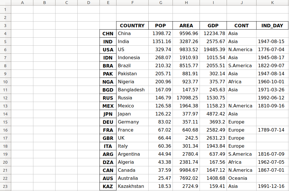
As you can see, the table starts in the third row 2 and the fifth column E.
.read_excel() also has the optional parameter sheet_name that specifies which worksheets to read when loading data. It can take on one of the following values:
- The zero-based index of the worksheet
- The name of the worksheet
- The list of indices or names to read multiple sheets
- The value
Noneto read all sheets
Here’s how you would use this parameter in your code:
>>>
>>> df = pd.read_excel('data.xlsx', sheet_name=0, index_col=0,
...                    parse_dates=['IND_DAY'])
>>> df = pd.read_excel('data.xlsx', sheet_name='COUNTRIES', index_col=0,
...                    parse_dates=['IND_DAY'])
Both statements above create the same DataFrame because the sheet_name parameters have the same values. In both cases, sheet_name=0 and sheet_name='COUNTRIES' refer to the same worksheet. The argument parse_dates=['IND_DAY'] tells pandas to try to consider the values in this column as dates or times.
There are other optional parameters you can use with .read_excel() and .to_excel() to determine the Excel engine, the encoding, the way to handle missing values and infinities, the method for writing column names and row labels, and so on.
SQL Files
pandas IO tools can also read and write databases. In this next example, you’ll write your data to a database called data.db. To get started, you’ll need the SQLAlchemy package. To learn more about it, you can read the official ORM tutorial. You’ll also need the database driver. Python has a built-in driver for SQLite.
You can install SQLAlchemy with pip:
You can also install it with Conda:
$ conda install sqlalchemy
Once you have SQLAlchemy installed, import create_engine() and create a database engine:
>>>
>>> from sqlalchemy import create_engine
>>> engine = create_engine('sqlite:///data.db', echo=False)
Now that you have everything set up, the next step is to create a DataFrame object. It’s convenient to specify the data types and apply .to_sql().
>>>
>>> dtypes = {'POP': 'float64', 'AREA': 'float64', 'GDP': 'float64',
...           'IND_DAY': 'datetime64'}
>>> df = pd.DataFrame(data=data).T.astype(dtype=dtypes)
>>> df.dtypes
COUNTRY            object
POP               float64
AREA              float64
GDP               float64
CONT               object
IND_DAY    datetime64[ns]
dtype: object
.astype() is a very convenient method you can use to set multiple data types at once.
Once you’ve created your DataFrame, you can save it to the database with .to_sql():
>>>
>>> df.to_sql('data.db', con=engine, index_label='ID')
The parameter con is used to specify the database connection or engine that you want to use. The optional parameter index_label specifies how to call the database column with the row labels. You’ll often see it take on the value ID, Id, or id.
You should get the database data.db with a single table that looks like this:
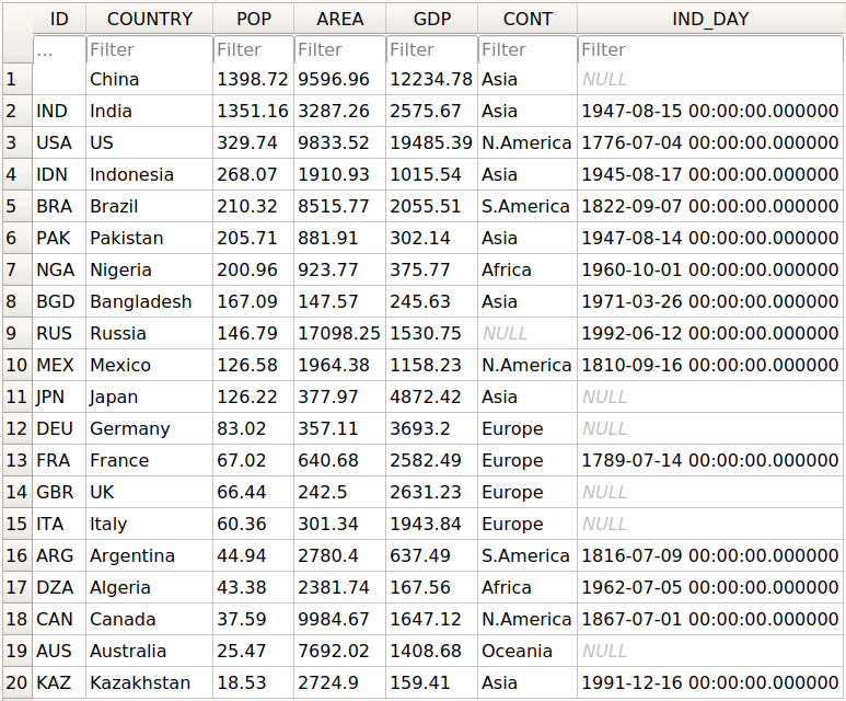
The first column contains the row labels. To omit writing them into the database, pass index=False to .to_sql(). The other columns correspond to the columns of the DataFrame.
There are a few more optional parameters. For example, you can use schema to specify the database schema and dtype to determine the types of the database columns. You can also use if_exists, which says what to do if a database with the same name and path already exists:
if_exists='fail'raises a ValueError and is the default.if_exists='replace'drops the table and inserts new values.if_exists='append'inserts new values into the table.
You can load the data from the database with read_sql():
>>>
>>> df = pd.read_sql('data.db', con=engine, index_col='ID')
>>> df
        COUNTRY      POP      AREA       GDP       CONT    IND_DAY
ID
CHN       China  1398.72   9596.96  12234.78       Asia        NaT
IND       India  1351.16   3287.26   2575.67       Asia 1947-08-15
USA          US   329.74   9833.52  19485.39  N.America 1776-07-04
IDN   Indonesia   268.07   1910.93   1015.54       Asia 1945-08-17
BRA      Brazil   210.32   8515.77   2055.51  S.America 1822-09-07
PAK    Pakistan   205.71    881.91    302.14       Asia 1947-08-14
NGA     Nigeria   200.96    923.77    375.77     Africa 1960-10-01
BGD  Bangladesh   167.09    147.57    245.63       Asia 1971-03-26
RUS      Russia   146.79  17098.25   1530.75       None 1992-06-12
MEX      Mexico   126.58   1964.38   1158.23  N.America 1810-09-16
JPN       Japan   126.22    377.97   4872.42       Asia        NaT
DEU     Germany    83.02    357.11   3693.20     Europe        NaT
FRA      France    67.02    640.68   2582.49     Europe 1789-07-14
GBR          UK    66.44    242.50   2631.23     Europe        NaT
ITA       Italy    60.36    301.34   1943.84     Europe        NaT
ARG   Argentina    44.94   2780.40    637.49  S.America 1816-07-09
DZA     Algeria    43.38   2381.74    167.56     Africa 1962-07-05
CAN      Canada    37.59   9984.67   1647.12  N.America 1867-07-01
AUS   Australia    25.47   7692.02   1408.68    Oceania        NaT
KAZ  Kazakhstan    18.53   2724.90    159.41       Asia 1991-12-16
The parameter index_col specifies the name of the column with the row labels. Note that this inserts an extra row after the header that starts with ID. You can fix this behavior with the following line of code:
>>>
>>> df.index.name = None
>>> df
        COUNTRY      POP      AREA       GDP       CONT    IND_DAY
CHN       China  1398.72   9596.96  12234.78       Asia        NaT
IND       India  1351.16   3287.26   2575.67       Asia 1947-08-15
USA          US   329.74   9833.52  19485.39  N.America 1776-07-04
IDN   Indonesia   268.07   1910.93   1015.54       Asia 1945-08-17
BRA      Brazil   210.32   8515.77   2055.51  S.America 1822-09-07
PAK    Pakistan   205.71    881.91    302.14       Asia 1947-08-14
NGA     Nigeria   200.96    923.77    375.77     Africa 1960-10-01
BGD  Bangladesh   167.09    147.57    245.63       Asia 1971-03-26
RUS      Russia   146.79  17098.25   1530.75       None 1992-06-12
MEX      Mexico   126.58   1964.38   1158.23  N.America 1810-09-16
JPN       Japan   126.22    377.97   4872.42       Asia        NaT
DEU     Germany    83.02    357.11   3693.20     Europe        NaT
FRA      France    67.02    640.68   2582.49     Europe 1789-07-14
GBR          UK    66.44    242.50   2631.23     Europe        NaT
ITA       Italy    60.36    301.34   1943.84     Europe        NaT
ARG   Argentina    44.94   2780.40    637.49  S.America 1816-07-09
DZA     Algeria    43.38   2381.74    167.56     Africa 1962-07-05
CAN      Canada    37.59   9984.67   1647.12  N.America 1867-07-01
AUS   Australia    25.47   7692.02   1408.68    Oceania        NaT
KAZ  Kazakhstan    18.53   2724.90    159.41       Asia 1991-12-16
Now you have the same DataFrame object as before.
Note that the continent for Russia is now None instead of nan. If you want to fill the missing values with nan, then you can use .fillna():
>>>
>>> df.fillna(value=float('nan'), inplace=True)
.fillna() replaces all missing values with whatever you pass to value. Here, you passed float('nan'), which says to fill all missing values with nan.
Also note that you didn’t have to pass parse_dates=['IND_DAY'] to read_sql(). That’s because your database was able to detect that the last column contains dates. However, you can pass parse_dates if you’d like. You’ll get the same results.
There are other functions that you can use to read databases, like read_sql_table() and read_sql_query(). Feel free to try them out!
Pickle Files
Pickling is the act of converting Python objects into byte streams. Unpickling is the inverse process. Python pickle files are the binary files that keep the data and hierarchy of Python objects. They usually have the extension .pickle or .pkl.
You can save your DataFrame in a pickle file with .to_pickle():
>>>
>>> dtypes = {'POP': 'float64', 'AREA': 'float64', 'GDP': 'float64',
...           'IND_DAY': 'datetime64'}
>>> df = pd.DataFrame(data=data).T.astype(dtype=dtypes)
>>> df.to_pickle('data.pickle')
Like you did with databases, it can be convenient first to specify the data types. Then, you create a file data.pickle to contain your data. You could also pass an integer value to the optional parameter protocol, which specifies the protocol of the pickler.
You can get the data from a pickle file with read_pickle():
>>>
>>> df = pd.read_pickle('data.pickle')
>>> df
        COUNTRY      POP      AREA       GDP       CONT    IND_DAY
CHN       China  1398.72   9596.96  12234.78       Asia        NaT
IND       India  1351.16   3287.26   2575.67       Asia 1947-08-15
USA          US   329.74   9833.52  19485.39  N.America 1776-07-04
IDN   Indonesia   268.07   1910.93   1015.54       Asia 1945-08-17
BRA      Brazil   210.32   8515.77   2055.51  S.America 1822-09-07
PAK    Pakistan   205.71    881.91    302.14       Asia 1947-08-14
NGA     Nigeria   200.96    923.77    375.77     Africa 1960-10-01
BGD  Bangladesh   167.09    147.57    245.63       Asia 1971-03-26
RUS      Russia   146.79  17098.25   1530.75        NaN 1992-06-12
MEX      Mexico   126.58   1964.38   1158.23  N.America 1810-09-16
JPN       Japan   126.22    377.97   4872.42       Asia        NaT
DEU     Germany    83.02    357.11   3693.20     Europe        NaT
FRA      France    67.02    640.68   2582.49     Europe 1789-07-14
GBR          UK    66.44    242.50   2631.23     Europe        NaT
ITA       Italy    60.36    301.34   1943.84     Europe        NaT
ARG   Argentina    44.94   2780.40    637.49  S.America 1816-07-09
DZA     Algeria    43.38   2381.74    167.56     Africa 1962-07-05
CAN      Canada    37.59   9984.67   1647.12  N.America 1867-07-01
AUS   Australia    25.47   7692.02   1408.68    Oceania        NaT
KAZ  Kazakhstan    18.53   2724.90    159.41       Asia 1991-12-16
read_pickle() returns the DataFrame with the stored data. You can also check the data types:
>>>
>>> df.dtypes
COUNTRY            object
POP               float64
AREA              float64
GDP               float64
CONT               object
IND_DAY    datetime64[ns]
dtype: object
These are the same ones that you specified before using .to_pickle().
As a word of caution, you should always beware of loading pickles from untrusted sources. This can be dangerous! When you unpickle an untrustworthy file, it could execute arbitrary code on your machine, gain remote access to your computer, or otherwise exploit your device in other ways.
Working With Big Data
If your files are too large for saving or processing, then there are several approaches you can take to reduce the required disk space:
- Compress your files
- Choose only the columns you want
- Omit the rows you don’t need
- Force the use of less precise data types
- Split the data into chunks
You’ll take a look at each of these techniques in turn.
Compress and Decompress Files
You can create an archive file like you would a regular one, with the addition of a suffix that corresponds to the desired compression type:
'.gz''.bz2''.zip''.xz'
pandas can deduce the compression type by itself:
>>>
>>> df = pd.DataFrame(data=data).T
>>> df.to_csv('data.csv.zip')
Here, you create a compressed .csv file as an archive. The size of the regular .csv file is 1048 bytes, while the compressed file only has 766 bytes.
You can open this compressed file as usual with the pandas read_csv() function:
>>>
>>> df = pd.read_csv('data.csv.zip', index_col=0,
...                  parse_dates=['IND_DAY'])
>>> df
        COUNTRY      POP      AREA       GDP       CONT    IND_DAY
CHN       China  1398.72   9596.96  12234.78       Asia        NaT
IND       India  1351.16   3287.26   2575.67       Asia 1947-08-15
USA          US   329.74   9833.52  19485.39  N.America 1776-07-04
IDN   Indonesia   268.07   1910.93   1015.54       Asia 1945-08-17
BRA      Brazil   210.32   8515.77   2055.51  S.America 1822-09-07
PAK    Pakistan   205.71    881.91    302.14       Asia 1947-08-14
NGA     Nigeria   200.96    923.77    375.77     Africa 1960-10-01
BGD  Bangladesh   167.09    147.57    245.63       Asia 1971-03-26
RUS      Russia   146.79  17098.25   1530.75        NaN 1992-06-12
MEX      Mexico   126.58   1964.38   1158.23  N.America 1810-09-16
JPN       Japan   126.22    377.97   4872.42       Asia        NaT
DEU     Germany    83.02    357.11   3693.20     Europe        NaT
FRA      France    67.02    640.68   2582.49     Europe 1789-07-14
GBR          UK    66.44    242.50   2631.23     Europe        NaT
ITA       Italy    60.36    301.34   1943.84     Europe        NaT
ARG   Argentina    44.94   2780.40    637.49  S.America 1816-07-09
DZA     Algeria    43.38   2381.74    167.56     Africa 1962-07-05
CAN      Canada    37.59   9984.67   1647.12  N.America 1867-07-01
AUS   Australia    25.47   7692.02   1408.68    Oceania        NaT
KAZ  Kazakhstan    18.53   2724.90    159.41       Asia 1991-12-16
read_csv() decompresses the file before reading it into a DataFrame.
You can specify the type of compression with the optional parameter compression, which can take on any of the following values:
'infer''gzip''bz2''zip''xz'None
The default value compression='infer' indicates that pandas should deduce the compression type from the file extension.
Here’s how you would compress a pickle file:
>>>
>>> df = pd.DataFrame(data=data).T
>>> df.to_pickle('data.pickle.compress', compression='gzip')
You should get the file data.pickle.compress that you can later decompress and read:
>>>
>>> df = pd.read_pickle('data.pickle.compress', compression='gzip')
df again corresponds to the DataFrame with the same data as before.
You can give the other compression methods a try, as well. If you’re using pickle files, then keep in mind that the .zip format supports reading only.
Choose Columns
The pandas read_csv() and read_excel() functions have the optional parameter usecols that you can use to specify the columns you want to load from the file. You can pass the list of column names as the corresponding argument:
>>>
>>> df = pd.read_csv('data.csv', usecols=['COUNTRY', 'AREA'])
>>> df
       COUNTRY      AREA
0        China   9596.96
1        India   3287.26
2           US   9833.52
3    Indonesia   1910.93
4       Brazil   8515.77
5     Pakistan    881.91
6      Nigeria    923.77
7   Bangladesh    147.57
8       Russia  17098.25
9       Mexico   1964.38
10       Japan    377.97
11     Germany    357.11
12      France    640.68
13          UK    242.50
14       Italy    301.34
15   Argentina   2780.40
16     Algeria   2381.74
17      Canada   9984.67
18   Australia   7692.02
19  Kazakhstan   2724.90
Now you have a DataFrame that contains less data than before. Here, there are only the names of the countries and their areas.
Instead of the column names, you can also pass their indices:
>>>
>>> df = pd.read_csv('data.csv',index_col=0, usecols=[0, 1, 3])
>>> df
        COUNTRY      AREA
CHN       China   9596.96
IND       India   3287.26
USA          US   9833.52
IDN   Indonesia   1910.93
BRA      Brazil   8515.77
PAK    Pakistan    881.91
NGA     Nigeria    923.77
BGD  Bangladesh    147.57
RUS      Russia  17098.25
MEX      Mexico   1964.38
JPN       Japan    377.97
DEU     Germany    357.11
FRA      France    640.68
GBR          UK    242.50
ITA       Italy    301.34
ARG   Argentina   2780.40
DZA     Algeria   2381.74
CAN      Canada   9984.67
AUS   Australia   7692.02
KAZ  Kazakhstan   2724.90
Expand the code block below to compare these results with the file 'data.csv':
,COUNTRY,POP,AREA,GDP,CONT,IND_DAY
CHN,China,1398.72,9596.96,12234.78,Asia,
IND,India,1351.16,3287.26,2575.67,Asia,1947-08-15
USA,US,329.74,9833.52,19485.39,N.America,1776-07-04
IDN,Indonesia,268.07,1910.93,1015.54,Asia,1945-08-17
BRA,Brazil,210.32,8515.77,2055.51,S.America,1822-09-07
PAK,Pakistan,205.71,881.91,302.14,Asia,1947-08-14
NGA,Nigeria,200.96,923.77,375.77,Africa,1960-10-01
BGD,Bangladesh,167.09,147.57,245.63,Asia,1971-03-26
RUS,Russia,146.79,17098.25,1530.75,,1992-06-12
MEX,Mexico,126.58,1964.38,1158.23,N.America,1810-09-16
JPN,Japan,126.22,377.97,4872.42,Asia,
DEU,Germany,83.02,357.11,3693.2,Europe,
FRA,France,67.02,640.68,2582.49,Europe,1789-07-14
GBR,UK,66.44,242.5,2631.23,Europe,
ITA,Italy,60.36,301.34,1943.84,Europe,
ARG,Argentina,44.94,2780.4,637.49,S.America,1816-07-09
DZA,Algeria,43.38,2381.74,167.56,Africa,1962-07-05
CAN,Canada,37.59,9984.67,1647.12,N.America,1867-07-01
AUS,Australia,25.47,7692.02,1408.68,Oceania,
KAZ,Kazakhstan,18.53,2724.9,159.41,Asia,1991-12-16
You can see the following columns:
- The column at index
0contains the row labels. - The column at index
1contains the country names. - The column at index
3contains the areas.
Simlarly, read_sql() has the optional parameter columns that takes a list of column names to read:
>>>
>>> df = pd.read_sql('data.db', con=engine, index_col='ID',
...                  columns=['COUNTRY', 'AREA'])
>>> df.index.name = None
>>> df
        COUNTRY      AREA
CHN       China   9596.96
IND       India   3287.26
USA          US   9833.52
IDN   Indonesia   1910.93
BRA      Brazil   8515.77
PAK    Pakistan    881.91
NGA     Nigeria    923.77
BGD  Bangladesh    147.57
RUS      Russia  17098.25
MEX      Mexico   1964.38
JPN       Japan    377.97
DEU     Germany    357.11
FRA      France    640.68
GBR          UK    242.50
ITA       Italy    301.34
ARG   Argentina   2780.40
DZA     Algeria   2381.74
CAN      Canada   9984.67
AUS   Australia   7692.02
KAZ  Kazakhstan   2724.90
Again, the DataFrame only contains the columns with the names of the countries and areas. If columns is None or omitted, then all of the columns will be read, as you saw before. The default behavior is columns=None.
Omit Rows
When you test an algorithm for data processing or machine learning, you often don’t need the entire dataset. It’s convenient to load only a subset of the data to speed up the process. The pandas read_csv() and read_excel() functions have some optional parameters that allow you to select which rows you want to load:
skiprows: either the number of rows to skip at the beginning of the file if it’s an integer, or the zero-based indices of the rows to skip if it’s a list-like objectskipfooter: the number of rows to skip at the end of the filenrows: the number of rows to read
Here’s how you would skip rows with odd zero-based indices, keeping the even ones:
>>>
>>> df = pd.read_csv('data.csv', index_col=0, skiprows=range(1, 20, 2))
>>> df
        COUNTRY      POP     AREA      GDP       CONT     IND_DAY
IND       India  1351.16  3287.26  2575.67       Asia  1947-08-15
IDN   Indonesia   268.07  1910.93  1015.54       Asia  1945-08-17
PAK    Pakistan   205.71   881.91   302.14       Asia  1947-08-14
BGD  Bangladesh   167.09   147.57   245.63       Asia  1971-03-26
MEX      Mexico   126.58  1964.38  1158.23  N.America  1810-09-16
DEU     Germany    83.02   357.11  3693.20     Europe         NaN
GBR          UK    66.44   242.50  2631.23     Europe         NaN
ARG   Argentina    44.94  2780.40   637.49  S.America  1816-07-09
CAN      Canada    37.59  9984.67  1647.12  N.America  1867-07-01
KAZ  Kazakhstan    18.53  2724.90   159.41       Asia  1991-12-16
In this example, skiprows is range(1, 20, 2) and corresponds to the values 1, 3, …, 19. The instances of the Python built-in class range behave like sequences. The first row of the file data.csv is the header row. It has the index 0, so pandas loads it in. The second row with index 1 corresponds to the label CHN, and pandas skips it. The third row with the index 2 and label IND is loaded, and so on.
If you want to choose rows randomly, then skiprows can be a list or NumPy array with pseudo-random numbers, obtained either with pure Python or with NumPy.
Force Less Precise Data Types
If you’re okay with less precise data types, then you can potentially save a significant amount of memory! First, get the data types with .dtypes again:
>>>
>>> df = pd.read_csv('data.csv', index_col=0, parse_dates=['IND_DAY'])
>>> df.dtypes
COUNTRY            object
POP               float64
AREA              float64
GDP               float64
CONT               object
IND_DAY    datetime64[ns]
dtype: object
The columns with the floating-point numbers are 64-bit floats. Each number of this type float64 consumes 64 bits or 8 bytes. Each column has 20 numbers and requires 160 bytes. You can verify this with .memory_usage():
>>>
>>> df.memory_usage()
Index      160
COUNTRY    160
POP        160
AREA       160
GDP        160
CONT       160
IND_DAY    160
dtype: int64
.memory_usage() returns an instance of Series with the memory usage of each column in bytes. You can conveniently combine it with .loc[] and .sum() to get the memory for a group of columns:
>>>
>>> df.loc[:, ['POP', 'AREA', 'GDP']].memory_usage(index=False).sum()
480
This example shows how you can combine the numeric columns 'POP', 'AREA', and 'GDP' to get their total memory requirement. The argument index=False excludes data for row labels from the resulting Series object. For these three columns, you’ll need 480 bytes.
You can also extract the data values in the form of a NumPy array with .to_numpy() or .values. Then, use the .nbytes attribute to get the total bytes consumed by the items of the array:
>>>
>>> df.loc[:, ['POP', 'AREA', 'GDP']].to_numpy().nbytes
480
The result is the same 480 bytes. So, how do you save memory?
In this case, you can specify that your numeric columns 'POP', 'AREA', and 'GDP' should have the type float32. Use the optional parameter dtype to do this:
>>>
>>> dtypes = {'POP': 'float32', 'AREA': 'float32', 'GDP': 'float32'}
>>> df = pd.read_csv('data.csv', index_col=0, dtype=dtypes,
...                  parse_dates=['IND_DAY'])
The dictionary dtypes specifies the desired data types for each column. It’s passed to the pandas read_csv() function as the argument that corresponds to the parameter dtype.
Now you can verify that each numeric column needs 80 bytes, or 4 bytes per item:
>>>
>>> df.dtypes
COUNTRY            object
POP               float32
AREA              float32
GDP               float32
CONT               object
IND_DAY    datetime64[ns]
dtype: object
>>> df.memory_usage()
Index      160
COUNTRY    160
POP         80
AREA        80
GDP         80
CONT       160
IND_DAY    160
dtype: int64
>>> df.loc[:, ['POP', 'AREA', 'GDP']].memory_usage(index=False).sum()
240
>>> df.loc[:, ['POP', 'AREA', 'GDP']].to_numpy().nbytes
240
Each value is a floating-point number of 32 bits or 4 bytes. The three numeric columns contain 20 items each. In total, you’ll need 240 bytes of memory when you work with the type float32. This is half the size of the 480 bytes you’d need to work with float64.
In addition to saving memory, you can significantly reduce the time required to process data by using float32 instead of float64 in some cases.
Use Chunks to Iterate Through Files
Another way to deal with very large datasets is to split the data into smaller chunks and process one chunk at a time. If you use read_csv(), read_json() or read_sql(), then you can specify the optional parameter chunksize:
>>>
>>> data_chunk = pd.read_csv('data.csv', index_col=0, chunksize=8)
>>> type(data_chunk)
<class 'pandas.io.parsers.TextFileReader'>
>>> hasattr(data_chunk, '__iter__')
True
>>> hasattr(data_chunk, '__next__')
True
chunksize defaults to None and can take on an integer value that indicates the number of items in a single chunk. When chunksize is an integer, read_csv() returns an iterable that you can use in a for loop to get and process only a fragment of the dataset in each iteration:
>>>
>>> for df_chunk in pd.read_csv('data.csv', index_col=0, chunksize=8):
...     print(df_chunk, end='nn')
...     print('memory:', df_chunk.memory_usage().sum(), 'bytes',
...           end='nnn')
...
        COUNTRY      POP     AREA       GDP       CONT     IND_DAY
CHN       China  1398.72  9596.96  12234.78       Asia         NaN
IND       India  1351.16  3287.26   2575.67       Asia  1947-08-15
USA          US   329.74  9833.52  19485.39  N.America  1776-07-04
IDN   Indonesia   268.07  1910.93   1015.54       Asia  1945-08-17
BRA      Brazil   210.32  8515.77   2055.51  S.America  1822-09-07
PAK    Pakistan   205.71   881.91    302.14       Asia  1947-08-14
NGA     Nigeria   200.96   923.77    375.77     Africa  1960-10-01
BGD  Bangladesh   167.09   147.57    245.63       Asia  1971-03-26

memory: 448 bytes


       COUNTRY     POP      AREA      GDP       CONT     IND_DAY
RUS     Russia  146.79  17098.25  1530.75        NaN  1992-06-12
MEX     Mexico  126.58   1964.38  1158.23  N.America  1810-09-16
JPN      Japan  126.22    377.97  4872.42       Asia         NaN
DEU    Germany   83.02    357.11  3693.20     Europe         NaN
FRA     France   67.02    640.68  2582.49     Europe  1789-07-14
GBR         UK   66.44    242.50  2631.23     Europe         NaN
ITA      Italy   60.36    301.34  1943.84     Europe         NaN
ARG  Argentina   44.94   2780.40   637.49  S.America  1816-07-09

memory: 448 bytes


        COUNTRY    POP     AREA      GDP       CONT     IND_DAY
DZA     Algeria  43.38  2381.74   167.56     Africa  1962-07-05
CAN      Canada  37.59  9984.67  1647.12  N.America  1867-07-01
AUS   Australia  25.47  7692.02  1408.68    Oceania         NaN
KAZ  Kazakhstan  18.53  2724.90   159.41       Asia  1991-12-16

memory: 224 bytes
In this example, the chunksize is 8. The first iteration of the for loop returns a DataFrame with the first eight rows of the dataset only. The second iteration returns another DataFrame with the next eight rows. The third and last iteration returns the remaining four rows.
In each iteration, you get and process the DataFrame with the number of rows equal to chunksize. It’s possible to have fewer rows than the value of chunksize in the last iteration. You can use this functionality to control the amount of memory required to process data and keep that amount reasonably small.
Conclusion
You now know how to save the data and labels from pandas DataFrame objects to different kinds of files. You also know how to load your data from files and create DataFrame objects.
You’ve used the pandas read_csv() and .to_csv() methods to read and write CSV files. You also used similar methods to read and write Excel, JSON, HTML, SQL, and pickle files. These functions are very convenient and widely used. They allow you to save or load your data in a single function or method call.
You’ve also learned how to save time, memory, and disk space when working with large data files:
- Compress or decompress files
- Choose the rows and columns you want to load
- Use less precise data types
- Split data into chunks and process them one by one
You’ve mastered a significant step in the machine learning and data science process! If you have any questions or comments, then please put them in the comments section below.
Watch Now This tutorial has a related video course created by the Real Python team. Watch it together with the written tutorial to deepen your understanding: Reading and Writing Files With Pandas
Узнайте, как читать и импортировать файлы Excel в Python, как записывать данные в эти таблицы и какие библиотеки лучше всего подходят для этого.
Известный вам инструмент для организации, анализа и хранения ваших данных в таблицах — Excel — применяется и в data science. В какой-то момент вам придется иметь дело с этими таблицами, но работать именно с ними вы будете не всегда. Вот почему разработчики Python реализовали способы чтения, записи и управления не только этими файлами, но и многими другими типами файлов.
Из этого учебника узнаете, как можете работать с Excel и Python. Внутри найдете обзор библиотек, которые вы можете использовать для загрузки и записи этих таблиц в файлы с помощью Python. Вы узнаете, как работать с такими библиотеками, как pandas, openpyxl, xlrd, xlutils и pyexcel.
Данные как ваша отправная точка
Когда вы начинаете проект по data science, вам придется работать с данными, которые вы собрали по всему интернету, и с наборами данных, которые вы загрузили из других мест — Kaggle, Quandl и тд
Но чаще всего вы также найдете данные в Google или в репозиториях, которые используются другими пользователями. Эти данные могут быть в файле Excel или сохранены в файл с расширением .csv … Возможности могут иногда казаться бесконечными, но когда у вас есть данные, в первую очередь вы должны убедиться, что они качественные.
В случае с электронной таблицей вы можете не только проверить, могут ли эти данные ответить на вопрос исследования, который вы имеете в виду, но также и можете ли вы доверять данным, которые хранятся в электронной таблице.
Проверяем качество таблицы
- Представляет ли электронная таблица статические данные?
- Смешивает ли она данные, расчеты и отчетность?
- Являются ли данные в вашей электронной таблице полными и последовательными?
- Имеет ли ваша таблица систематизированную структуру рабочего листа?
- Проверяли ли вы действительные формулы в электронной таблице?
Этот список вопросов поможет убедиться, что ваша таблица не грешит против лучших практик, принятых в отрасли. Конечно, этот список не исчерпывающий, но позволит провести базовую проверку таблицы.
Лучшие практики для данных электронных таблиц
Прежде чем приступить к чтению вашей электронной таблицы на Python, вы также должны подумать о том, чтобы настроить свой файл в соответствии с некоторыми основными принципами, такими как:
- Первая строка таблицы обычно зарезервирована для заголовка, а первый столбец используется для идентификации единицы выборки;
- Избегайте имен, значений или полей с пробелами. В противном случае каждое слово будет интерпретироваться как отдельная переменная, что приведет к ошибкам, связанным с количеством элементов на строку в вашем наборе данных. По возможности, используйте:
- подчеркивания,
- тире,
- горбатый регистр, где первая буква каждого слова пишется с большой буквы
- объединяющие слова
- Короткие имена предпочтительнее длинных имен;
- старайтесь не использовать имена, которые содержат символы ?, $,%, ^, &, *, (,), -, #,? ,,, <,>, /, |, , [,], {, и };
- Удалите все комментарии, которые вы сделали в вашем файле, чтобы избежать добавления в ваш файл лишних столбцов или NA;
- Убедитесь, что все пропущенные значения в вашем наборе данных обозначены как NA.
Затем, после того, как вы внесли необходимые изменения или тщательно изучили свои данные, убедитесь, что вы сохранили внесенные изменения. Сделав это, вы можете вернуться к данным позже, чтобы отредактировать их, добавить дополнительные данные или изменить их, сохранив формулы, которые вы, возможно, использовали для расчета данных и т.д.
Если вы работаете с Microsoft Excel, вы можете сохранить файл в разных форматах: помимо расширения по умолчанию .xls или .xlsx, вы можете перейти на вкладку «Файл», нажать «Сохранить как» и выбрать одно из расширений, которые указаны в качестве параметров «Сохранить как тип». Наиболее часто используемые расширения для сохранения наборов данных в data science — это .csv и .txt (в виде текстового файла с разделителями табуляции). В зависимости от выбранного варианта сохранения поля вашего набора данных разделяются вкладками или запятыми, которые образуют символы-разделители полей вашего набора данных.
Теперь, когда вы проверили и сохранили ваши данные, вы можете начать с подготовки вашего рабочего окружения.
Готовим рабочее окружение
Как убедиться, что вы все делаете хорошо? Проверить рабочее окружение!
Когда вы работаете в терминале, вы можете сначала перейти в каталог, в котором находится ваш файл, а затем запустить Python. Убедитесь, что файл лежит именно в том каталоге, к которому вы обратились.
Возможно, вы уже начали сеанс Python и у вас нет подсказок о каталоге, в котором вы работаете. Тогда можно выполнить следующие команды:
# Import `os`
import os

# Retrieve current working directory (`cwd`)
cwd = os.getcwd()
cwd

# Change directory
os.chdir("/path/to/your/folder")

# List all files and directories in current directory
os.listdir('.')
Круто, да?
Вы увидите, что эти команды очень важны не только для загрузки ваших данных, но и для дальнейшего анализа. А пока давайте продолжим: вы прошли все проверки, вы сохранили свои данные и подготовили рабочее окружение.
Можете ли вы начать с чтения данных в Python?
Установите библиотеки для чтения и записи файлов Excel
Даже если вы еще не знаете, какие библиотеки вам понадобятся для импорта ваших данных, вы должны убедиться, что у вас есть все, что нужно для установки этих библиотек, когда придет время.
Подготовка к дополнительной рабочей области: pip
Вот почему вам нужно установить pip и setuptools. Если у вас установлен Python2 ⩾ 2.7.9 или Python3 ⩾ 3.4, то можно не беспокоиться — просто убедитесь, что вы обновились до последней версии.
Для этого выполните следующую команду в своем терминале:
# Для Linux/OS X
pip install -U pip setuptools

# Для Windows
python -m pip install -U pip setuptools
Если вы еще не установили pip, запустите скрипт python get-pip.py, который вы можете найти здесь. Следуйте инструкциям по установке.
Установка Anaconda
Другой вариант для работы в data science — установить дистрибутив Anaconda Python. Сделав это, вы получите простой и быстрый способ начать заниматься data science, потому что вам не нужно беспокоиться об установке отдельных библиотек, необходимых для работы.
Это особенно удобно, если вы новичок, но даже для более опытных разработчиков это способ быстро протестировать некоторые вещи без необходимости устанавливать каждую библиотеку отдельно.
Anaconda включает в себя 100 самых популярных библиотек Python, R и Scala для науки о данных и несколько сред разработки с открытым исходным кодом, таких как Jupyter и Spyder.
Установить Anaconda можно здесь. Следуйте инструкциям по установке, и вы готовы начать!
Загрузить файлы Excel в виде фреймов Pandas
Все, среда настроена, вы готовы начать импорт ваших файлов.
Один из способов, который вы часто используете для импорта ваших файлов для обработки данных, — с помощью библиотеки Pandas. Она основана на NumPy и предоставляет простые в использовании структуры данных и инструменты анализа данных Python.
Эта мощная и гибкая библиотека очень часто используется дата-инженерами для передачи своих данных в структуры данных, очень выразительных для их анализа.
Если у вас уже есть Pandas, доступные через Anaconda, вы можете просто загрузить свои файлы в Pandas DataFrames с помощью pd.Excelfile():
# импорт библиотеки pandas
import pandas as pd

# Загружаем ваш файл в переменную `file` / вместо 'example' укажите название свого файла из текущей директории
file = 'example.xlsx'

# Загружаем spreadsheet в объект pandas
xl = pd.ExcelFile(file)

# Печатаем название листов в данном файле
print(xl.sheet_names)

# Загрузить лист в DataFrame по его имени: df1
df1 = xl.parse('Sheet1')
Если вы не установили Anaconda, просто выполните pip install pandas, чтобы установить библиотеку Pandas в вашей среде, а затем выполните команды, которые включены в фрагмент кода выше.
Проще простого, да?
Для чтения в файлах .csv у вас есть аналогичная функция для загрузки данных в DataFrame: read_csv(). Вот пример того, как вы можете использовать эту функцию:
# Импорт библиотеки pandas
import pandas as pd

# Загрузить csv файл
df = pd.read_csv("example.csv")
Разделитель, который будет учитывать эта функция, по умолчанию является запятой, но вы можете указать альтернативный разделитель, если хотите. Перейдите к документации, чтобы узнать, какие другие аргументы вы можете указать для успешного импорта!
Обратите внимание, что есть также функции read_table() и read_fwf() для чтения файлов и таблиц с фиксированной шириной в формате DataFrames с общим разделителем. Для первой функции разделителем по умолчанию является вкладка, но вы можете снова переопределить это, а также указать альтернативный символ-разделитель. Более того, есть и другие функции, которые вы можете использовать для получения данных в DataFrames: вы можете найти их здесь.
Как записать Pandas DataFrames в файлы Excel
Допустим, что после анализа данных вы хотите записать данные обратно в новый файл. Есть также способ записать ваши Pandas DataFrames обратно в файлы с помощью функции to_excel().
Но, прежде чем использовать эту функцию, убедитесь, что у вас установлен XlsxWriter, если вы хотите записать свои данные в несколько листов в файле .xlsx:
# Установим `XlsxWriter`
pip install XlsxWriter

# Указать writer библиотеки
writer = pd.ExcelWriter('example.xlsx', engine='xlsxwriter')

# Записать ваш DataFrame в файл
yourData.to_excel(writer, 'Sheet1')

# Сохраним результат
writer.save()
Обратите внимание, что в приведенном выше фрагменте кода вы используете объект ExcelWriter для вывода DataFrame.
Иными словами, вы передаете переменную Writer в функцию to_excel() и также указываете имя листа. Таким образом, вы добавляете лист с данными в существующую рабочую книгу: вы можете использовать ExcelWriter для сохранения нескольких (немного) разных DataFrames в одной рабочей книге.
Все это означает, что если вы просто хотите сохранить один DataFrame в файл, вы также можете обойтись без установки пакета XlsxWriter. Затем вы просто не указываете аргумент движка, который вы передаете в функцию pd.ExcelWriter(). Остальные шаги остаются прежними.
Аналогично функциям, которые вы использовали для чтения в файлах .csv, у вас также есть функция to_csv() для записи результатов обратно в файл, разделенный запятыми. Он снова работает так же, как когда вы использовали его для чтения в файле:
# Запишите DataFrame в csv
df.to_csv("example.csv")
Если вы хотите иметь файл, разделенный табуляцией, вы также можете передать t аргументу sep. Обратите внимание, что есть другие функции, которые вы можете использовать для вывода ваших файлов. Вы можете найти их все здесь.
Пакеты для разбора файлов Excel и обратной записи с помощью Python
Помимо библиотеки Pandas, который вы будете использовать очень часто для загрузки своих данных, вы также можете использовать другие библиотеки для получения ваших данных в Python. Наш обзор основан на этой странице со списком доступных библиотек, которые вы можете использовать для работы с файлами Excel в Python.
Далее вы увидите, как использовать эти библиотеки с помощью некоторых реальных, но упрощенных примеров.
Использование виртуальных сред
Общий совет для установки — делать это в Python virtualenv без системных пакетов. Вы можете использовать virtualenv для создания изолированных сред Python: он создает папку, содержащую все необходимые исполняемые файлы для использования пакетов, которые потребуются проекту Python.
Чтобы начать работать с virtualenv, вам сначала нужно установить его. Затем перейдите в каталог, в который вы хотите поместить свой проект. Создайте virtualenv в этой папке и загрузите в определенную версию Python, если вам это нужно. Затем вы активируете виртуальную среду. После этого вы можете начать загрузку в другие библиотеки, начать работать с ними и т. д.
Совет: не забудьте деактивировать среду, когда закончите!
# Install virtualenv
$ pip install virtualenv

# Go to the folder of your project
$ cd my_folder

# Create a virtual environment `venv`
$ virtualenv venv

# Indicate the Python interpreter to use for `venv`
$ virtualenv -p /usr/bin/python2.7 venv

# Activate `venv`
$ source venv/bin/activate

# Deactivate `venv`
$ deactivate
Обратите внимание, что виртуальная среда может показаться немного проблемной на первый взгляд, когда вы только начинаете работать с данными с Python. И, особенно если у вас есть только один проект, вы можете не понять, зачем вам вообще нужна виртуальная среда.
С ней будет гораздо легче, когда у вас одновременно запущено несколько проектов, и вы не хотите, чтобы они использовали одну и ту же установку Python. Или когда ваши проекты имеют противоречащие друг другу требования, виртуальная среда пригодится!
Теперь вы можете, наконец, начать установку и импорт библиотек, о которых вы читали, и загрузить их в таблицу.
Как читать и записывать файлы Excel с openpyxl
Этот пакет обычно рекомендуется, если вы хотите читать и записывать файлы .xlsx, xlsm, xltx и xltm.
Установите openpyxl с помощью pip: вы видели, как это сделать в предыдущем разделе.
Общий совет для установки этой библиотеки — делать это в виртуальной среде Python без системных библиотек. Вы можете использовать виртуальную среду для создания изолированных сред Python: она создает папку, которая содержит все необходимые исполняемые файлы для использования библиотек, которые потребуются проекту Python.
Перейдите в каталог, в котором находится ваш проект, и повторно активируйте виртуальную среду venv. Затем продолжите установку openpyxl с pip, чтобы убедиться, что вы можете читать и записывать файлы с ним:
# Активируйте virtualenv
$ source activate venv

# Установим `openpyxl` в `venv`
$ pip install openpyxl
Теперь, когда вы установили openpyxl, вы можете загружать данные. Но что это за данные?
Доспутим Excel с данными, которые вы пытаетесь загрузить в Python, содержит следующие листы:
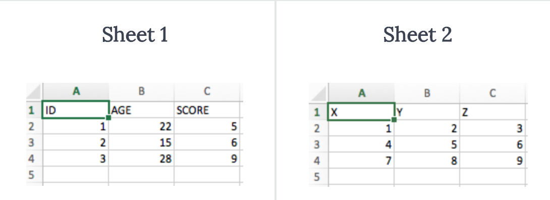
Функция load_workbook() принимает имя файла в качестве аргумента и возвращает объект рабочей книги, который представляет файл. Вы можете проверить это, запустив type (wb). Убедитесь, что вы находитесь в том каталоге, где находится ваша таблица, иначе вы получите error при импорте.
# Import `load_workbook` module from `openpyxl`
from openpyxl import load_workbook

# Load in the workbook
wb = load_workbook('./test.xlsx')

# Get sheet names
print(wb.get_sheet_names())
Помните, что вы можете изменить рабочий каталог с помощью os.chdir().
Вы видите, что фрагмент кода выше возвращает имена листов книги, загруженной в Python.Можете использовать эту информацию, чтобы также получить отдельные листы рабочей книги.
Вы также можете проверить, какой лист в настоящее время активен с wb.active. Как видно из кода ниже, вы можете использовать его для загрузки другого листа из вашей книги:
# Get a sheet by name
sheet = wb.get_sheet_by_name('Sheet3')

# Print the sheet title
sheet.title

# Get currently active sheet
anotherSheet = wb.active

# Check `anotherSheet`
anotherSheet
На первый взгляд, с этими объектами рабочего листа вы не сможете многое сделать.. Однако вы можете извлечь значения из определенных ячеек на листе вашей книги, используя квадратные скобки [], в которые вы передаете точную ячейку, из которой вы хотите получить значение.
Обратите внимание, что это похоже на выбор, получение и индексирование массивов NumPy и Pandas DataFrames, но это не все, что вам нужно сделать, чтобы получить значение. Вам нужно добавить атрибут value:
# Retrieve the value of a certain cell
sheet['A1'].value

# Select element 'B2' of your sheet
c = sheet['B2']

# Retrieve the row number of your element
c.row

# Retrieve the column letter of your element
c.column

# Retrieve the coordinates of the cell
c.coordinate
Как вы можете видеть, помимо значения, есть и другие атрибуты, которые вы можете использовать для проверки вашей ячейки, а именно: row, column и coordinate.
Атрибут row вернет 2;
Добавление атрибута column к c даст вам ‘B’
coordinate вернет ‘B2’.
Вы также можете получить значения ячеек с помощью функции cell(). Передайте row и column, добавьте к этим аргументам значения, соответствующие значениям ячейки, которую вы хотите получить, и, конечно же, не забудьте добавить атрибут value:
# Retrieve cell value
sheet.cell(row=1, column=2).value

# Print out values in column 2
for i in range(1, 4):
     print(i, sheet.cell(row=i, column=2).value)
Обратите внимание, что если вы не укажете атрибут value, вы получите <Cell Sheet3.B1>, который ничего не говорит о значении, которое содержится в этой конкретной ячейке.
Вы видите, что вы используете цикл for с помощью функции range(), чтобы помочь вам распечатать значения строк, имеющих значения в столбце 2. Если эти конкретные ячейки пусты, вы просто вернете None. Если вы хотите узнать больше о циклах for, пройдите наш курс Intermediate Python для Data Science.
Есть специальные функции, которые вы можете вызывать для получения некоторых других значений, например, get_column_letter() и column_index_from_string.
Две функции указывают примерно то, что вы можете получить, используя их, но лучше сделать их четче: хотя вы можете извлечь букву столбца с предшествующего, вы можете сделать обратное или получить адрес столбца, когда вы задаёте букву последнему. Вы можете увидеть, как это работает ниже:
# Импорт необходимых модулей из  `openpyxl.utils`
from openpyxl.utils import get_column_letter, column_index_from_string

# Вывод 'A'
get_column_letter(1)

# Return '1'
column_index_from_string('A')
Вы уже получили значения для строк, которые имеют значения в определенном столбце, но что вам нужно сделать, если вы хотите распечатать строки вашего файла, не сосредотачиваясь только на одном столбце? Использовать другой цикл, конечно!
Например, вы говорите, что хотите сфокусироваться на области между «А1» и «С3», где первая указывает на левый верхний угол, а вторая — на правый нижний угол области, на которой вы хотите сфокусироваться. ,
Эта область будет так называемым cellObj, который вы видите в первой строке кода ниже. Затем вы говорите, что для каждой ячейки, которая находится в этой области, вы печатаете координату и значение, которое содержится в этой ячейке. После конца каждой строки вы печатаете сообщение, которое указывает, что строка этой области cellObj напечатана.
# Напечатать строчку за строчкой
for cellObj in sheet['A1':'C3']:
      for cell in cellObj:
              print(cells.coordinate, cells.value)
      print('--- END ---')
Еще раз обратите внимание, что выбор области очень похож на выбор, получение и индексирование списка и элементов массива NumPy, где вы также используете [] и : для указания области, значения которой вы хотите получить. Кроме того, вышеприведенный цикл также хорошо использует атрибуты ячейки!
Чтобы сделать вышеприведенное объяснение и код наглядным, вы можете проверить результат, который вы получите после завершения цикла:
('A1', u'M')
('B1', u'N')
('C1', u'O')
--- END ---
('A2', 10L)
('B2', 11L)
('C2', 12L)
--- END ---
('A3', 14L)
('B3', 15L)
('C3', 16L)
--- END ---
Наконец, есть некоторые атрибуты, которые вы можете использовать для проверки результата вашего импорта, а именно max_row и max_column. Эти атрибуты, конечно, и так — общие способы проверки правильности загрузки данных, но они все равно полезны.
# Вывести максимальное количество строк
sheet.max_row

# Вывести максимальное количество колонок
sheet.max_column
Наверное, вы думаете, что такой способ работы с этими файлами сложноват, особенно если вы еще хотите манипулировать данными.
Должно быть что-то попроще, верно? Так и есть!
openpyxl поддерживает Pandas DataFrames! Вы можете использовать функцию DataFrame() из библиотеки Pandas, чтобы поместить значения листа в DataFrame:
# Import `pandas`
import pandas as pd

# конвертировать Лист в DataFrame
df = pd.DataFrame(sheet.values)
Если вы хотите указать заголовки и индексы, вам нужно добавить немного больше кода:
# Put the sheet values in `data`
data = sheet.values

# Indicate the columns in the sheet values
cols = next(data)[1:]

# Convert your data to a list
data = list(data)

# Read in the data at index 0 for the indices
idx = [r[0] for r in data]

# Slice the data at index 1
data = (islice(r, 1, None) for r in data)

# Make your DataFrame
df = pd.DataFrame(data, index=idx, columns=cols)
Затем вы можете начать манипулировать данными со всеми функциями, которые предлагает библиотека Pandas. Но помните, что вы находитесь в виртуальной среде, поэтому, если библиотека еще не представлена, вам нужно будет установить ее снова через pip.
Чтобы записать ваши Pandas DataFrames обратно в файл Excel, вы можете легко использовать функцию dataframe_to_rows() из модуля utils:
# Import `dataframe_to_rows`
from openpyxl.utils.dataframe import dataframe_to_rows

# Initialize a workbook
wb = Workbook()

# Get the worksheet in the active workbook
ws = wb.active

# Append the rows of the DataFrame to your worksheet
for r in dataframe_to_rows(df, index=True, header=True):
    ws.append(r)
Но это точно не все! Библиотека openpyxl предлагает вам высокую гибкость при записи ваших данных обратно в файлы Excel, изменении стилей ячеек или использовании режима write-only. Эту библиотеку обязательно нужно знать, когда вы часто работаете с электронными таблицами ,
Совет: читайте больше о том, как вы можете изменить стили ячеек, перейти в режим write-only или как библиотека работает с NumPy здесь.
Теперь давайте также рассмотрим некоторые другие библиотеки, которые вы можете использовать для получения данных вашей электронной таблицы в Python.
Прежде чем закрыть этот раздел, не забудьте отключить виртуальную среду, когда закончите!
Чтение и форматирование Excel-файлов: xlrd
Эта библиотека идеально подходит для чтения и форматирования данных из Excel с расширением xls или xlsx.
# Import `xlrd`
import xlrd

# Open a workbook
workbook = xlrd.open_workbook('example.xls')

# Loads only current sheets to memory
workbook = xlrd.open_workbook('example.xls', on_demand = True)
Когда вам не нужны данные из всей Excel-книги, вы можете использовать функции sheet_by_name() или sheet_by_index() для получения листов, которые вы хотите получить в своём анализе
# Load a specific sheet by name
worksheet = workbook.sheet_by_name('Sheet1')

# Load a specific sheet by index
worksheet = workbook.sheet_by_index(0)

# Retrieve the value from cell at indices (0,0)
sheet.cell(0, 0).value
Также можно получить значение в определённых ячейках с вашего листа.
Перейдите к xlwt и xlutils, чтобы узнать больше о том, как они относятся к библиотеке xlrd.
Запись данных в Excel-файлы с xlwt
Если вы хотите создать таблицу со своими данными, вы можете использовать не только библиотеку XlsWriter, но и xlwt. xlwt идеально подходит для записи данных и форматирования информации в файлах с расширением .xls
Когда вы вручную создаёте файл:
# Import `xlwt`
import xlwt

# Initialize a workbook
book = xlwt.Workbook(encoding="utf-8")

# Add a sheet to the workbook
sheet1 = book.add_sheet("Python Sheet 1")

# Write to the sheet of the workbook
sheet1.write(0, 0, "This is the First Cell of the First Sheet")

# Save the workbook
book.save("spreadsheet.xls")
Если вы хотите записать данные в файл, но не хотите делать все самостоятельно, вы всегда можете прибегнуть к циклу for, чтобы автоматизировать весь процесс. Составьте сценарий, в котором вы создаёте книгу и в которую добавляете лист. Укажите список со столбцами и один со значениями, которые будут заполнены на листе.
Далее у вас есть цикл for, который гарантирует, что все значения попадают в файл: вы говорите, что для каждого элемента в диапазоне от 0 до 4 (5 не включительно) вы собираетесь что-то делать. Вы будете заполнять значения построчно. Для этого вы указываете элемент строки, который появляется в каждом цикле. Далее у вас есть еще один цикл for, который будет проходить по столбцам вашего листа. Вы говорите, что для каждой строки на листе, вы будете смотреть на столбцы, которые идут с ним, и вы будете заполнять значение для каждого столбца в строке. Заполнив все столбцы строки значениями, вы перейдете к следующей строке, пока не останется строк.
# Initialize a workbook
book = xlwt.Workbook()

# Add a sheet to the workbook
sheet1 = book.add_sheet("Sheet1")

# The data
cols = ["A", "B", "C", "D", "E"]
txt = [0,1,2,3,4]

# Loop over the rows and columns and fill in the values
for num in range(5):
      row = sheet1.row(num)
      for index, col in enumerate(cols):
          value = txt[index] + num
          row.write(index, value)

# Save the result
book.save("test.xls")
На скриншоте ниже представлен результат выполнения этого кода:
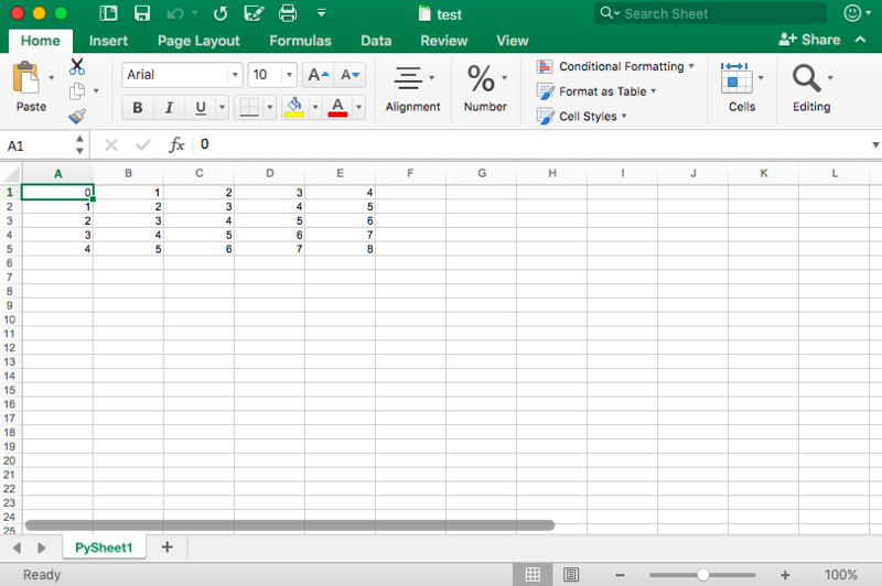
Теперь, когда вы увидели, как xlrd и xlwt работают друг с другом, пришло время взглянуть на библиотеку, которая тесно связана с этими двумя: xlutils.
Сборник утилит: xlutils
Эта библиотека — сборник утилит, для которого требуются и xlrd и xlwt, и которая может копировать, изменять и фильтровать существующие данные. О том, как пользоваться этими командами рассказано в разделе по openpyxl.
Вернитесь в раздел openpyxl, чтобы получить больше информации о том, как использовать этот пакет для получения данных в Python.
Использование pyexcel для чтения .xls или .xlsx файлов
Еще одна библиотека, которую можно использовать для чтения данных электронных таблиц в Python — это pyexcel; Python Wrapper, который предоставляет один API для чтения, записи и работы с данными в файлах .csv, .ods, .xls, .xlsx и .xlsm. Конечно, для этого урока вы просто сосредоточитесь на файлах .xls и .xls.
Чтобы получить ваши данные в массиве, вы можете использовать функцию get_array(), которая содержится в пакете pyexcel:
# Import `pyexcel`
import pyexcel

# Get an array from the data
my_array = pyexcel.get_array(file_name="test.xls")
Вы также можете получить свои данные в упорядоченном словаре списков. Вы можете использовать функцию get_dict():
# Import `OrderedDict` module
from pyexcel._compact import OrderedDict

# Get your data in an ordered dictionary of lists
my_dict = pyexcel.get_dict(file_name="test.xls", name_columns_by_row=0)

# Get your data in a dictionary of 2D arrays
book_dict = pyexcel.get_book_dict(file_name="test.xls")
Здесь видно, что если вы хотите получить словарь двумерных массивов или получить все листы рабочей книги в одном словаре, вы можете прибегнуть к get_book_dict().
Помните, что эти две структуры данных, которые были упомянуты выше, массивы и словари вашей таблицы, позволяют вам создавать DataFrames ваших данных с помощью pd.DataFrame(). Это облегчит обработку данных.
Кроме того, вы можете просто получить записи из таблицы с помощью pyexcel благодаря функции get_records(). Просто передайте аргумент file_name в функцию, и вы получите список словарей:
# Retrieve the records of the file
records = pyexcel.get_records(file_name="test.xls")
Чтобы узнать, как управлять списками Python, ознакомьтесь с примерами из документации о списках Python.
Запись в файл с pyexcel
С помощью этой библиотеки можно не только загружать данные в массивы, вы также можете экспортировать свои массивы обратно в таблицу. Используйте функцию save_as() и передайте массив и имя файла назначения в аргумент dest_file_name:
# Get the data
data = [[1, 2, 3], [4, 5, 6], [7, 8, 9]]

# Save the array to a file
pyexcel.save_as(array=data, dest_file_name="array_data.xls")
Обратите внимание, что если вы хотите указать разделитель, вы можете добавить аргумент dest_delimiter и передать символ, который вы хотите использовать в качестве разделителя между «».
Однако если у вас есть словарь, вам нужно использовать функцию save_book_as(). Передайте двумерный словарь в bookdict и укажите имя файла:
# The data
2d_array_dictionary = {'Sheet 1': [
                                   ['ID', 'AGE', 'SCORE']
                                   [1, 22, 5],
                                   [2, 15, 6],
                                   [3, 28, 9]
                                  ],
                       'Sheet 2': [
                                    ['X', 'Y', 'Z'],
                                    [1, 2, 3],
                                    [4, 5, 6]
                                    [7, 8, 9]
                                  ],
                       'Sheet 3': [
                                    ['M', 'N', 'O', 'P'],
                                    [10, 11, 12, 13],
                                    [14, 15, 16, 17]
                                    [18, 19, 20, 21]
                                   ]}

# Save the data to a file
pyexcel.save_book_as(bookdict=2d_array_dictionary, dest_file_name="2d_array_data.xls")
При использовании кода, напечатанного в приведенном выше примере, важно помнить, что порядок ваших данных в словаре не будет сохранен. Если вы не хотите этого, вам нужно сделать небольшой обход. Вы можете прочитать все об этом здесь.
Чтение и запись .csv файлов
Если вы все еще ищете библиотеки, которые позволяют загружать и записывать данные в файлы .csv, кроме Pandas, лучше всего использовать пакет csv:
# import `csv`
import csv

# Read in csv file
for row in csv.reader(open('data.csv'), delimiter=','):
      print(row)

# Write csv file
data = [[1, 2, 3], [4, 5, 6], [7, 8, 9]]
outfile = open('data.csv', 'w')
writer = csv.writer(outfile, delimiter=';', quotechar='"')
writer.writerows(data)
outfile.close()
Обратите внимание, что в пакете NumPy есть функция genfromtxt(), которая позволяет загружать данные, содержащиеся в файлах .csv, в массивы, которые затем можно поместить в DataFrames.
Финальная проверка данных
Когда у вас есть данные, не забудьте последний шаг: проверить, правильно ли загружены данные. Если вы поместили свои данные в DataFrame, вы можете легко и быстро проверить, был ли импорт успешным, выполнив следующие команды:
# Check the first entries of the DataFrame
df1.head()

# Check the last entries of the DataFrame
df1.tail()
Если у вас есть данные в массиве, вы можете проверить их, используя следующие атрибуты массива: shape, ndim, dtype и т.д .:
# Inspect the shape
data.shape

# Inspect the number of dimensions
data.ndim

# Inspect the data type
data.dtype
Что дальше?
Поздравляем! Вы успешно прошли наш урок и научились читать файлы Excel на Python.
Если вы хотите продолжить работу над этой темой, попробуйте воспользоваться PyXll, который позволяет писать функции в Python и вызывать их в Excel.
Earlier is showed you how to use the Python CSV library to read and write to CSV files. While CSV does work, and I still use elements of it occasionally, you will find working with Pandas to be so much easier.
Practice Files Excel: Linear Regression Example File 1
CSV: heightWeight_w_headers
Let’s start with our CSV file. Unzip it and place it in a folder where you will be able to find it.
If you want to make your life a little easier, when you open your Jupyter Notebook, type pwd
This will give you your present working directory. If you place your csv file in this directory, all you have to do is call it by name.

I am not going to do that however. I want to show you how to work with directories.
Get Full Directory Path
For Windows Users, if you hold down the Shift key while right clicking on your file, you will see an option that says: Copy as Path

Read the CSV file
First import pandas as pd
Then assign a variable = pd.read_csv(file name) – paste the full path of your CSV file here.
variable.head() = the first 5 rows from your data frame.

Write CSV file
Okay, let’s write a CSV file. First, let’s add some rows to current dataframe.
We will do this be first creating a new dataframe with 3 rows of data.

Now we will use the .append() function to append this new dataframe to end of our existing dataframe.
The ignore_index = True argument tells the new rows to continue using the index of the main dataframe. Otherwise, the new rows would start counting at 0 again. If you want to try it, just leave out the argument: HgtWgt_df.append(df2)

Now, we just use the df.to_csv() command to write our appended dataframe to a new CSV file

And there is our new file

Read Excel File
I’d love to be able to wow you with how complicated reading an Excel file is, but the difference between the Excel file reading and CSV is one word – excel.

The only caveat is if your Excel file has multiple sheets. By default pd.read_excel() goes to sheet 1. If you want it to read sheet 4 instead, you would add: pd.read_excel(filename, sheetname= 4)
Write to Excel File

Bonus note
If you haven’t already, please check out my earlier CSV lesson: Python: Working with CSV Files
This will really give you an appreciation for how powerful and time saving pandas really is.
If you enjoyed this lesson, click LIKE below, or even better, leave me a COMMENT.
Follow this link for more Python content: Python