
The read_excel() method can read Excel 2003 (.xls) and
Excel 2007+ (.xlsx) files using the xlrd Python
module. The to_excel() instance method is used for
saving a DataFrame to Excel. Generally the semantics are
similar to working with csv data. See the cookbook for some
advanced strategies
10.5.1 Reading Excel Files
In the most basic use-case, read_excel takes a path to an Excel
file, and the sheetname indicating which sheet to parse.
# Returns a DataFrame
read_excel('path_to_file.xls', sheetname='Sheet1')
10.5.1.1 ExcelFile class
To facilitate working with multiple sheets from the same file, the ExcelFile
class can be used to wrap the file and can be be passed into read_excel
There will be a performance benefit for reading multiple sheets as the file is
read into memory only once.
xlsx = pd.ExcelFile('path_to_file.xls)
df = pd.read_excel(xlsx, 'Sheet1')
The ExcelFile class can also be used as a context manager.
with pd.ExcelFile('path_to_file.xls') as xls:
    df1 = pd.read_excel(xls, 'Sheet1')
    df2 = pd.read_excel(xls, 'Sheet2')
The sheet_names property will generate
a list of the sheet names in the file.
The primary use-case for an ExcelFile is parsing multiple sheets with
different parameters
data = {}
# For when Sheet1's format differs from Sheet2
with pd.ExcelFile('path_to_file.xls') as xls:
    data['Sheet1'] = pd.read_excel(xls, 'Sheet1', index_col=None, na_values=['NA'])
    data['Sheet2'] = pd.read_excel(xls, 'Sheet2', index_col=1)
Note that if the same parsing parameters are used for all sheets, a list
of sheet names can simply be passed to read_excel with no loss in performance.
# using the ExcelFile class
data = {}
with pd.ExcelFile('path_to_file.xls') as xls:
    data['Sheet1'] = read_excel(xls, 'Sheet1', index_col=None, na_values=['NA'])
    data['Sheet2'] = read_excel(xls, 'Sheet2', index_col=None, na_values=['NA'])

# equivalent using the read_excel function
data = read_excel('path_to_file.xls', ['Sheet1', 'Sheet2'], index_col=None, na_values=['NA'])
New in version 0.12.
ExcelFile has been moved to the top level namespace.
New in version 0.17.
read_excel can take an ExcelFile object as input
10.5.1.2 Specifying Sheets
Note
The second argument is sheetname, not to be confused with ExcelFile.sheet_names
Note
An ExcelFile’s attribute sheet_names provides access to a list of sheets.
- The arguments
sheetnameallows specifying the sheet or sheets to read. - The default value for
sheetnameis 0, indicating to read the first sheet - Pass a string to refer to the name of a particular sheet in the workbook.
- Pass an integer to refer to the index of a sheet. Indices follow Python
convention, beginning at 0. - Pass a list of either strings or integers, to return a dictionary of specified sheets.
- Pass a
Noneto return a dictionary of all available sheets.
# Returns a DataFrame
read_excel('path_to_file.xls', 'Sheet1', index_col=None, na_values=['NA'])
Using the sheet index:
# Returns a DataFrame
read_excel('path_to_file.xls', 0, index_col=None, na_values=['NA'])
Using all default values:
# Returns a DataFrame
read_excel('path_to_file.xls')
Using None to get all sheets:
# Returns a dictionary of DataFrames
read_excel('path_to_file.xls',sheetname=None)
Using a list to get multiple sheets:
# Returns the 1st and 4th sheet, as a dictionary of DataFrames.
read_excel('path_to_file.xls',sheetname=['Sheet1',3])
New in version 0.16.
read_excel can read more than one sheet, by setting sheetname to either
a list of sheet names, a list of sheet positions, or None to read all sheets.
New in version 0.13.
Sheets can be specified by sheet index or sheet name, using an integer or string,
respectively.
10.5.1.3 Reading a MultiIndex
New in version 0.17.
read_excel can read a MultiIndex index, by passing a list of columns to index_col
and a MultiIndex column by passing a list of rows to header. If either the index
or columns have serialized level names those will be read in as well by specifying
the rows/columns that make up the levels.
For example, to read in a MultiIndex index without names:
In [1]: df = pd.DataFrame({'a':[1,2,3,4], 'b':[5,6,7,8]},
   ...:                   index=pd.MultiIndex.from_product([['a','b'],['c','d']]))
   ...:

In [2]: df.to_excel('path_to_file.xlsx')

In [3]: df = pd.read_excel('path_to_file.xlsx', index_col=[0,1])

In [4]: df
Out[4]:
     a  b
a c  1  5
  d  2  6
b c  3  7
  d  4  8
If the index has level names, they will parsed as well, using the same
parameters.
In [5]: df.index = df.index.set_names(['lvl1', 'lvl2'])

In [6]: df.to_excel('path_to_file.xlsx')

In [7]: df = pd.read_excel('path_to_file.xlsx', index_col=[0,1])

In [8]: df
Out[8]:
           a  b
lvl1 lvl2
a    c     1  5
     d     2  6
b    c     3  7
     d     4  8
If the source file has both MultiIndex index and columns, lists specifying each
should be passed to index_col and header
In [9]: df.columns = pd.MultiIndex.from_product([['a'],['b', 'd']], names=['c1', 'c2'])

In [10]: df.to_excel('path_to_file.xlsx')

In [11]: df = pd.read_excel('path_to_file.xlsx',
   ....:                     index_col=[0,1], header=[0,1])
   ....:

In [12]: df
Out[12]:
c1         a
c2         b  d
lvl1 lvl2
a    c     1  5
     d     2  6
b    c     3  7
     d     4  8
Warning
Excel files saved in version 0.16.2 or prior that had index names will still able to be read in,
but the has_index_names argument must specified to True.
10.5.1.4 Parsing Specific Columns
It is often the case that users will insert columns to do temporary computations
in Excel and you may not want to read in those columns. read_excel takes
a parse_cols keyword to allow you to specify a subset of columns to parse.
If parse_cols is an integer, then it is assumed to indicate the last column
to be parsed.
read_excel('path_to_file.xls', 'Sheet1', parse_cols=2)
If parse_cols is a list of integers, then it is assumed to be the file column
indices to be parsed.
read_excel('path_to_file.xls', 'Sheet1', parse_cols=[0, 2, 3])
10.5.1.5 Cell Converters
It is possible to transform the contents of Excel cells via the converters
option. For instance, to convert a column to boolean:
read_excel('path_to_file.xls', 'Sheet1', converters={'MyBools': bool})
This options handles missing values and treats exceptions in the converters
as missing data. Transformations are applied cell by cell rather than to the
column as a whole, so the array dtype is not guaranteed. For instance, a
column of integers with missing values cannot be transformed to an array
with integer dtype, because NaN is strictly a float. You can manually mask
missing data to recover integer dtype:
cfun = lambda x: int(x) if x else -1
read_excel('path_to_file.xls', 'Sheet1', converters={'MyInts': cfun})
10.5.2 Writing Excel Files
10.5.2.1 Writing Excel Files to Disk
To write a DataFrame object to a sheet of an Excel file, you can use the
to_excel instance method. The arguments are largely the same as to_csv
described above, the first argument being the name of the excel file, and the
optional second argument the name of the sheet to which the DataFrame should be
written. For example:
df.to_excel('path_to_file.xlsx', sheet_name='Sheet1')
Files with a .xls extension will be written using xlwt and those with a
.xlsx extension will be written using xlsxwriter (if available) or
openpyxl.
The DataFrame will be written in a way that tries to mimic the REPL output. One
difference from 0.12.0 is that the index_label will be placed in the second
row instead of the first. You can get the previous behaviour by setting the
merge_cells option in to_excel() to False:
df.to_excel('path_to_file.xlsx', index_label='label', merge_cells=False)
The Panel class also has a to_excel instance method,
which writes each DataFrame in the Panel to a separate sheet.
In order to write separate DataFrames to separate sheets in a single Excel file,
one can pass an ExcelWriter.
with ExcelWriter('path_to_file.xlsx') as writer:
    df1.to_excel(writer, sheet_name='Sheet1')
    df2.to_excel(writer, sheet_name='Sheet2')
Note
Wringing a little more performance out of read_excel
Internally, Excel stores all numeric data as floats. Because this can
produce unexpected behavior when reading in data, pandas defaults to trying
to convert integers to floats if it doesn’t lose information (1.0 -->). You can pass
1convert_float=False to disable this behavior, which
may give a slight performance improvement.
10.5.2.2 Writing Excel Files to Memory
New in version 0.17.
Pandas supports writing Excel files to buffer-like objects such as StringIO or
BytesIO using ExcelWriter.
New in version 0.17.
Added support for Openpyxl >= 2.2
# Safe import for either Python 2.x or 3.x
try:
    from io import BytesIO
except ImportError:
    from cStringIO import StringIO as BytesIO

bio = BytesIO()

# By setting the 'engine' in the ExcelWriter constructor.
writer = ExcelWriter(bio, engine='xlsxwriter')
df.to_excel(writer, sheet_name='Sheet1')

# Save the workbook
writer.save()

# Seek to the beginning and read to copy the workbook to a variable in memory
bio.seek(0)
workbook = bio.read()
Note
engine is optional but recommended. Setting the engine determines
the version of workbook produced. Setting engine='xlrd' will produce an
Excel 2003-format workbook (xls). Using either 'openpyxl' or
'xlsxwriter' will produce an Excel 2007-format workbook (xlsx). If
omitted, an Excel 2007-formatted workbook is produced.
10.5.3 Excel writer engines
New in version 0.13.
pandas chooses an Excel writer via two methods:
- the
enginekeyword argument - the filename extension (via the default specified in config options)
By default, pandas uses the XlsxWriter for .xlsx and openpyxl
for .xlsm files and xlwt for .xls files. If you have multiple
engines installed, you can set the default engine through setting the
config options io.excel.xlsx.writer and
io.excel.xls.writer. pandas will fall back on openpyxl for .xlsx
files if Xlsxwriter is not available.
To specify which writer you want to use, you can pass an engine keyword
argument to to_excel and to ExcelWriter. The built-in engines are:
openpyxl: This includes stable support for Openpyxl from 1.6.1. However,
it is advised to use version 2.2 and higher, especially when working with
styles.xlsxwriterxlwt
# By setting the 'engine' in the DataFrame and Panel 'to_excel()' methods.
df.to_excel('path_to_file.xlsx', sheet_name='Sheet1', engine='xlsxwriter')

# By setting the 'engine' in the ExcelWriter constructor.
writer = ExcelWriter('path_to_file.xlsx', engine='xlsxwriter')

# Or via pandas configuration.
from pandas import options
options.io.excel.xlsx.writer = 'xlsxwriter'

df.to_excel('path_to_file.xlsx', sheet_name='Sheet1')
In this tutorial, you’ll learn how to use Python and Pandas to read Excel files using the Pandas read_excel function. Excel files are everywhere – and while they may not be the ideal data type for many data scientists, knowing how to work with them is an essential skill.
By the end of this tutorial, you’ll have learned:
- How to use the Pandas read_excel function to read an Excel file
- How to read specify an Excel sheet name to read into Pandas
- How to read multiple Excel sheets or files
- How to certain columns from an Excel file in Pandas
- How to skip rows when reading Excel files in Pandas
- And more
Let’s get started!
The Quick Answer: Use Pandas read_excel to Read Excel Files
To read Excel files in Python’s Pandas, use the read_excel() function. You can specify the path to the file and a sheet name to read, as shown below:
# Reading an Excel File in Pandas
import pandas as pd

df = pd.read_excel('/Users/datagy/Desktop/Sales.xlsx')

# With a Sheet Name
df = pd.read_excel(
   io='/Users/datagy/Desktop/Sales.xlsx'
   sheet_name ='North'
)
In the following sections of this tutorial, you’ll learn more about the Pandas read_excel() function to better understand how to customize reading Excel files.
Understanding the Pandas read_excel Function
The Pandas read_excel() function has a ton of different parameters. In this tutorial, you’ll learn how to use the main parameters available to you that provide incredible flexibility in terms of how you read Excel files in Pandas.
| Parameter | Description | Available Option |
|---|---|---|
io= |
The string path to the workbook. | URL to file, path to file, etc. |
sheet_name= |
The name of the sheet to read. Will default to the first sheet in the workbook (position 0). | Can read either strings (for the sheet name), integers (for position), or lists (for multiple sheets) |
usecols= |
The columns to read, if not all columns are to be read | Can be strings of columns, Excel-style columns (“A:C”), or integers representing positions columns |
dtype= |
The datatypes to use for each column | Dictionary with columns as keys and data types as values |
skiprows= |
The number of rows to skip from the top | Integer value representing the number of rows to skip |
nrows= |
The number of rows to parse | Integer value representing the number of rows to read |
.read_excel() functionThe table above highlights some of the key parameters available in the Pandas .read_excel() function. The full list can be found in the official documentation. In the following sections, you’ll learn how to use the parameters shown above to read Excel files in different ways using Python and Pandas.
As shown above, the easiest way to read an Excel file using Pandas is by simply passing in the filepath to the Excel file. The io= parameter is the first parameter, so you can simply pass in the string to the file.
The parameter accepts both a path to a file, an HTTP path, an FTP path or more. Let’s see what happens when we read in an Excel file hosted on my Github page.
# Reading an Excel file in Pandas
import pandas as pd

df = pd.read_excel('https://github.com/datagy/mediumdata/raw/master/Sales.xlsx')
print(df.head())

# Returns:
#         Date Customer  Sales
# 0 2022-04-01        A    191
# 1 2022-04-02        B    727
# 2 2022-04-03        A    782
# 3 2022-04-04        B    561
# 4 2022-04-05        A    969
If you’ve downloaded the file and taken a look at it, you’ll notice that the file has three sheets? So, how does Pandas know which sheet to load? By default, Pandas will use the first sheet (positionally), unless otherwise specified.
In the following section, you’ll learn how to specify which sheet you want to load into a DataFrame.
How to Specify Excel Sheet Names in Pandas read_excel
As shown in the previous section, you learned that when no sheet is specified, Pandas will load the first sheet in an Excel workbook. In the workbook provided, there are three sheets in the following structure:
Sales.xlsx
|---East
|---West
|---North
Because of this, we know that the data from the sheet “East” was loaded. If we wanted to load the data from the sheet “West”, we can use the sheet_name= parameter to specify which sheet we want to load.
The parameter accepts both a string as well as an integer. If we were to pass in a string, we can specify the sheet name that we want to load.
Let’s take a look at how we can specify the sheet name for 'West':
# Specifying an Excel Sheet to Load by Name
import pandas as pd

df = pd.read_excel(
    io='https://github.com/datagy/mediumdata/raw/master/Sales.xlsx',
    sheet_name='West')
print(df.head())

# Returns:
#         Date Customer  Sales
# 0 2022-04-01        A    504
# 1 2022-04-02        B    361
# 2 2022-04-03        A    694
# 3 2022-04-04        B    702
# 4 2022-04-05        A    255
Similarly, we can load a sheet name by its position. By default, Pandas will use the position of 0, which will load the first sheet. Say we wanted to repeat our earlier example and load the data from the sheet named 'West', we would need to know where the sheet is located.
Because we know the sheet is the second sheet, we can pass in the 1st index:
# Specifying an Excel Sheet to Load by Position
import pandas as pd

df = pd.read_excel(
    io='https://github.com/datagy/mediumdata/raw/master/Sales.xlsx',
    sheet_name=1)
print(df.head())

# Returns:
#         Date Customer  Sales
# 0 2022-04-01        A    504
# 1 2022-04-02        B    361
# 2 2022-04-03        A    694
# 3 2022-04-04        B    702
# 4 2022-04-05        A    255
We can see that both of these methods returned the same sheet’s data. In the following section, you’ll learn how to specify which columns to load when using the Pandas read_excel function.
How to Specify Columns Names in Pandas read_excel
There may be many times when you don’t want to load every column in an Excel file. This may be because the file has too many columns or has different columns for different worksheets.
In order to do this, we can use the usecols= parameter. It’s a very flexible parameter that lets you specify:
- A list of column names,
- A string of Excel column ranges,
- A list of integers specifying the column indices to load
Most commonly, you’ll encounter people using a list of column names to read in. Each of these columns are comma separated strings, contained in a list.
Let’s load our DataFrame from the example above, only this time only loading the 'Customer' and 'Sales' columns:
# Specifying Columns to Load by Name
import pandas as pd

df = pd.read_excel(
    io='https://github.com/datagy/mediumdata/raw/master/Sales.xlsx',
    usecols=['Customer', 'Sales'])
print(df.head())

# Returns:
#   Customer  Sales
# 0        A    191
# 1        B    727
# 2        A    782
# 3        B    561
# 4        A    969
We can see that by passing in the list of strings representing the columns, we were able to parse those columns only.
If we wanted to use Excel changes, we could also specify columns 'B:C'. Let’s see what this looks like below:
# Specifying Columns to Load by Excel Range
import pandas as pd

df = pd.read_excel(
    io='https://github.com/datagy/mediumdata/raw/master/Sales.xlsx',
    usecols='B:C')
print(df.head())

# Returns:
#   Customer  Sales
# 0        A    191
# 1        B    727
# 2        A    782
# 3        B    561
# 4        A    969
Finally, we can also pass in a list of integers that represent the positions of the columns we wanted to load. Because the columns are the second and third columns, we would load a list of integers as shown below:
# Specifying Columns to Load by Their Position
import pandas as pd

df = pd.read_excel(
    io='https://github.com/datagy/mediumdata/raw/master/Sales.xlsx',
    usecols=[1,2])
print(df.head())

# Returns:
#   Customer  Sales
# 0        A    191
# 1        B    727
# 2        A    782
# 3        B    561
# 4        A    969
In the following section, you’ll learn how to specify data types when reading Excel files.
How to Specify Data Types in Pandas read_excel
Pandas makes it easy to specify the data type of different columns when reading an Excel file. This serves three main purposes:
- Preventing data from being read incorrectly
- Speeding up the read operation
- Saving memory
You can pass in a dictionary where the keys are the columns and the values are the data types. This ensures that data are ready correctly. Let’s see how we can specify the data types for our columns.
# Specifying Data Types for Columns When Reading Excel Files
import pandas as pd

df = pd.read_excel(
    io='https://github.com/datagy/mediumdata/raw/master/Sales.xlsx',
    dtype={'date':'datetime64', 'Customer': 'object', 'Sales':'int'})
print(df.head())

# Returns:
#   Customer  Sales
#         Date Customer  Sales
# 0 2022-04-01        A    191
# 1 2022-04-02        B    727
# 2 2022-04-03        A    782
# 3 2022-04-04        B    561
# 4 2022-04-05        A    969
It’s important to note that you don’t need to pass in all the columns for this to work. In the next section, you’ll learn how to skip rows when reading Excel files.
How to Skip Rows When Reading Excel Files in Pandas
In some cases, you’ll encounter files where there are formatted title rows in your Excel file, as shown below:
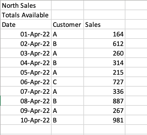
If we were to read the sheet 'North', we would get the following returned:
# Reading a poorly formatted Excel file
import pandas as pd

df = pd.read_excel(
    io='https://github.com/datagy/mediumdata/raw/master/Sales.xlsx',
    sheet_name='North')
print(df.head())

# Returns:
#            North Sales Unnamed: 1 Unnamed: 2
# 0     Totals Available        NaN        NaN
# 1                 Date   Customer      Sales
# 2  2022-04-01 00:00:00          A        164
# 3  2022-04-02 00:00:00          B        612
# 4  2022-04-03 00:00:00          A        260
Pandas makes it easy to skip a certain number of rows when reading an Excel file. This can be done using the skiprows= parameter. We can see that we need to skip two rows, so we can simply pass in the value 2, as shown below:
# Reading a Poorly Formatted File Correctly
import pandas as pd

df = pd.read_excel(
    io='https://github.com/datagy/mediumdata/raw/master/Sales.xlsx',
    sheet_name='North',
    skiprows=2)
print(df.head())

# Returns:
#         Date Customer  Sales
# 0 2022-04-01        A    164
# 1 2022-04-02        B    612
# 2 2022-04-03        A    260
# 3 2022-04-04        B    314
# 4 2022-04-05        A    215
This read the file much more accurately! It can be a lifesaver when working with poorly formatted files. In the next section, you’ll learn how to read multiple sheets in an Excel file in Pandas.
How to Read Multiple Sheets in an Excel File in Pandas
Pandas makes it very easy to read multiple sheets at the same time. This can be done using the sheet_name= parameter. In our earlier examples, we passed in only a single string to read a single sheet. However, you can also pass in a list of sheets to read multiple sheets at once.
Let’s see how we can read our first two sheets:
# Reading Multiple Excel Sheets at Once in Pandas
import pandas as pd

dfs = pd.read_excel(
    io='https://github.com/datagy/mediumdata/raw/master/Sales.xlsx',
    sheet_name=['East', 'West'])

print(type(dfs))

# Returns: <class 'dict'>
In the example above, we passed in a list of sheets to read. When we used the type() function to check the type of the returned value, we saw that a dictionary was returned.
Each of the sheets is a key of the dictionary with the DataFrame being the corresponding key’s value. Let’s see how we can access the 'West' DataFrame:
# Reading Multiple Excel Sheets in Pandas
import pandas as pd

dfs = pd.read_excel(
    io='https://github.com/datagy/mediumdata/raw/master/Sales.xlsx',
    sheet_name=['East', 'West'])

print(dfs.get('West').head())

# Returns:
#         Date Customer  Sales
# 0 2022-04-01        A    504
# 1 2022-04-02        B    361
# 2 2022-04-03        A    694
# 3 2022-04-04        B    702
# 4 2022-04-05        A    255
You can also read all of the sheets at once by specifying None for the value of sheet_name=. Similarly, this returns a dictionary of all sheets:
# Reading Multiple Excel Sheets in Pandas
import pandas as pd

dfs = pd.read_excel(
    io='https://github.com/datagy/mediumdata/raw/master/Sales.xlsx',
    sheet_name=None)
In the next section, you’ll learn how to read multiple Excel files in Pandas.
How to Read Only n Lines When Reading Excel Files in Pandas
When working with very large Excel files, it can be helpful to only sample a small subset of the data first. This allows you to quickly load the file to better be able to explore the different columns and data types.
This can be done using the nrows= parameter, which accepts an integer value of the number of rows you want to read into your DataFrame. Let’s see how we can read the first five rows of the Excel sheet:
# Reading n Number of Rows of an Excel Sheet
import pandas as pd

df = pd.read_excel(
    io='https://github.com/datagy/mediumdata/raw/master/Sales.xlsx',
    nrows=5)
print(df)

# Returns:
#         Date Customer  Sales
# 0 2022-04-01        A    191
# 1 2022-04-02        B    727
# 2 2022-04-03        A    782
# 3 2022-04-04        B    561
# 4 2022-04-05        A    969
Conclusion
In this tutorial, you learned how to use Python and Pandas to read Excel files into a DataFrame using the .read_excel() function. You learned how to use the function to read an Excel, specify sheet names, read only particular columns, and specify data types. You then learned how skip rows, read only a set number of rows, and read multiple sheets.
Additional Resources
To learn more about related topics, check out the tutorials below:
- Pandas Dataframe to CSV File – Export Using .to_csv()
- Combine Data in Pandas with merge, join, and concat
- Introduction to Pandas for Data Science
- Summarizing and Analyzing a Pandas DataFrame
pandas.read_excel() function is used to read excel sheet with extension xlsx into pandas DataFrame. By reading a single sheet it returns a pandas DataFrame object, but reading two sheets it returns a Dict of DataFrame.
pandas Read Excel Key Points
- This supports to read files with extension xls, xlsx, xlsm, xlsb, odf, ods and odt
- Can load excel files stored in a local filesystem or from an URL.
- For URL, it supports http, ftp, s3, and file.
- Also supports reading from a single sheet or a list of sheets.
- When reading a two sheets, it returns a Dict of DataFrame.
Table of contents –
- Read Excel Sheet into DataFrame
- Read by Ignoring Column Names
- Set Column from Excel as Index
- Read Excel by Sheet Name
- Read Two Sheets
- Skip Columns From Excel
- Skip Rows From Excel
- Other Important Params
I have an excel file with two sheets named Technologies and Schedule, I will be using this to demonstrate how to read into pandas DataFrame.
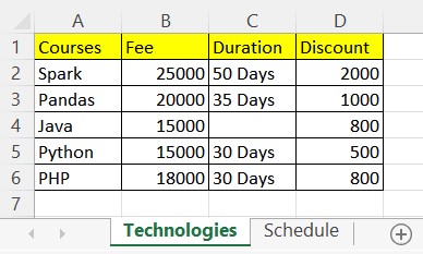

Notice that on our excel file the top row contains the header of the table which can be used as column names on DataFrame.
1. pandas Read Excel Sheet
Use pandas.read_excel() function to read excel sheet into pandas DataFrame, by default it loads the first sheet from the excel file and parses the first row as a DataFrame column name. Excel file has an extension .xlsx. This function also supports several extensions xls, xlsx, xlsm, xlsb, odf, ods and odt .
Following are some of the features supported by read_excel() with optional param.
- Reading excel file from URL, S3, and from local file ad supports several extensions.
- Ignoreing the column names and provides an option to set column names.
- Setting column as Index
- Considering multiple values as NaN
- Decimal points to use for numbers
- Data types for each column
- Skipping rows and columns
I will cover how to use some of these optional params with examples, first let’s see how to read an excel sheet & create a DataFrame without any params.
import pandas as pd
# Read Excel file
df = pd.read_excel('c:/apps/courses_schedule.xlsx')
print(df)

# Outputs
#   Courses    Fee  Duration  Discount
#0    Spark  25000   50 Days      2000
#1   Pandas  20000   35 Days      1000
#2     Java  15000       NaN       800
#3   Python  15000   30 Days       500
#4      PHP  18000   30 Days       800
Related: pandas Write to Excel Sheet
By default, it considers the first row from excel as a header and used it as DataFrame column names. In case you wanted to consider the first row from excel as a data record use header=None param and use names param to specify the column names. Not specifying names result in column names with numerical numbers.
# Read excel by considering first row as data
columns = ['courses','course_fee','course_duration','course_discount']
df2 = pd.read_excel('c:/apps/courses_schedule.xlsx',
                   header=None, names = columns)
print(df2)

# Outputs
#0  courses  course_fee  Duration  Discount
#1    Spark  25000   50 Days      2000
#2   Pandas  20000   35 Days      1000
#3     Java  15000       NaN       800
#4   Python  15000   30 Days       500
#5      PHP  18000   30 Days       800
3. Set Column from Excel as Index
If you notice, the DataFrame was created with the default index, if you wanted to set the column name as index use index_col param. This param takes values {int, list of int, default None}. If a list is passed with header positions, it creates a MultiIndex.
By default, it is set to None meaning not column is set as an index.
# Read excel by setting column as index
df2 = pd.read_excel('c:/apps/courses_schedule.xlsx',
                   index_col=0)
print(df2)

# Outputs
#           Fee Duration  Discount
#Courses
#Spark    25000  50 Days      2000
#Pandas   20000  35 Days      1000
#Java     15000      NaN       800
#Python   15000  30 Days       500
#PHP      18000  30 Days       800
4. Read Excel by Sheet Name
As I said in the above section by default pandas read the first sheet from the excel file and provide a sheet_name param to read a specific sheet by name. This param takes {str, int, list, or None} as values. This is also used to load a sheet by position.
By default, it is set to 0 meaning load the first sheet.
# Read specific excel sheet
df = pd.read_excel('records.xlsx', sheet_name='Sheet1')
print(df)
5. Read Two Sheets
sheet_name param also takes a list of sheet names as values that can be used to read two sheets into pandas DataFrame. Not that while reading two sheets it returns a Dict of DataFrame. The key in Dict is a sheet name and the value would be DataFrame.
Use None to load all sheets from excel and returns a Dict of Dictionary.
# Read Multiple sheets
dict_df = pd.read_excel('c:/apps/courses_schedule.xlsx',
                   sheet_name=['Technologies','Schedule'])

# Get DataFrame from Dict
technologies_df = dict_df .get('Technologies')
schedule_df = dict_df.get('Schedule')

# Print DataFrame's
print(technologies_df)
print(schedule_df)
I will leave this to you to execute and validate the output.
6. Skip Columns From Excel Sheet
Sometimes while reading an excel sheet into pandas DataFrame you may need to skip columns, you can do this by using usecols param. This takes values {int, str, list-like, or callable default None}. To specify the list of column names or positions use a list of strings or a list of int.
By default it is set to None meaning load all columns
# Read excel by skipping columns
df2 = pd.read_excel('c:/apps/courses_schedule.xlsx',
                   usecols=['Courses', 'Duration'])
print(df2)
# Outputs
#  Courses Duration
#0   Spark  50 Days
#1  Pandas  35 Days
#2    Java      NaN
#3  Python  30 Days
#4     PHP  30 Days
Alternatively, you can also write it by column position.
# Skip columns with list of values
df = pd.read_excel('records.xlsx', usecols=[0,2])
print(df)
Also supports a range of columns as value. For example, value ‘B:D’ means parsing B, C, and D columns.
# Skip columns by range
df2 = pd.read_excel('c:/apps/courses_schedule.xlsx',
                   usecols='B:D')
print(df2)

     Fee Duration  Discount
0  25000  50 Days      2000
1  20000  35 Days      1000
2  15000      NaN       800
3  15000  30 Days       500
4  18000  30 Days       800
7. Skip Rows from Excel Sheet
Use skiprows param to skip rows from the excel file, this param takes values {list-like, int, or callable, optional}. With this, you can skip the first few rows, selected rows, and range of rows. The below example skips the first 3 rows and considers the 4th row from excel as the header.
# Read excel file by skipping rows
df2 = pd.read_excel('c:/apps/courses_schedule.xlsx',
                   skiprows=2)
print(df2)

   Pandas  20000  35 Days  1000
0    Java  15000      NaN   800
1  Python  15000  30 Days   500
2     PHP  18000  30 Days   800
Use header=None to consider the 4th row as data. you can also use a list of rows to skip.
# Using skiprows to skip rows
df2 = pd.read_excel('c:/apps/courses_schedule.xlsx',
                   skiprows=[1,3])
print(df2)

  Courses    Fee Duration  Discount
0  Pandas  20000  35 Days      1000
1  Python  15000  30 Days       500
2     PHP  18000  30 Days       800
By using a lambda expression.
# Using skiprows with lambda
df2 = pd.read_excel('c:/apps/courses_schedule.xlsx',
                   skiprows=lambda x: x in [1,3])
print(df2)
8. Other Important Params
- dtype – Dict with column name an type.
- nrows – How many rows to parse.
- na_values – Additional strings to recognize as NA/NaN.
- keep_default_na – Whether or not to include the default NaN values when parsing the data.
- na_filter – Filters missing values.
- parse_dates – Specify the column index you wanted to parse as dates
- thousands – Thousands separator for parsing string columns to numeric.
- skipfooter – Specify how to rows you wanted to skip from the footer.
- mangle_dupe_cols – Duplicate columns will be specified as ‘X’, ‘X.1’, …’X.N’,
For complete params and description, refer to pandas documentation.
Conclusion
In this article, you have learned how to read an Excel sheet and covert it into DataFrame by ignoring header, skipping rows, skipping columns, specifying column names, and many more.
Happy Learning !!
Related Articles
- pandas ExcelWriter Usage with Examples
- pandas write CSV file
- Pandas Read SQL Query or Table with Examples
- Pandas Read TSV with Examples
- Pandas Read Text with Examples
- Pandas read_csv() with Examples
- Pandas Read JSON File with Examples
- How to Read CSV from String in Pandas
- Pandas Write to Excel with Examples
References
- https://docs.microsoft.com/en-us/deployoffice/compat/office-file-format-reference
- https://en.wikipedia.org/wiki/List_of_Microsoft_Office_filename_extensions
.. currentmodule:: pandas
IO tools (text, CSV, HDF5, …)
The pandas I/O API is a set of top level reader functions accessed like
:func:`pandas.read_csv` that generally return a pandas object. The corresponding
writer functions are object methods that are accessed like
:meth:`DataFrame.to_csv`. Below is a table containing available readers and
writers.
| Format Type | Data Description | Reader | Writer |
|---|---|---|---|
| text | CSV | :ref:`read_csv<io.read_csv_table>` | :ref:`to_csv<io.store_in_csv>` |
| text | Fixed-Width Text File | :ref:`read_fwf<io.fwf_reader>` | |
| text | JSON | :ref:`read_json<io.json_reader>` | :ref:`to_json<io.json_writer>` |
| text | HTML | :ref:`read_html<io.read_html>` | :ref:`to_html<io.html>` |
| text | LaTeX | :ref:`Styler.to_latex<io.latex>` | |
| text | XML | :ref:`read_xml<io.read_xml>` | :ref:`to_xml<io.xml>` |
| text | Local clipboard | :ref:`read_clipboard<io.clipboard>` | :ref:`to_clipboard<io.clipboard>` |
| binary | MS Excel | :ref:`read_excel<io.excel_reader>` | :ref:`to_excel<io.excel_writer>` |
| binary | OpenDocument | :ref:`read_excel<io.ods>` | |
| binary | HDF5 Format | :ref:`read_hdf<io.hdf5>` | :ref:`to_hdf<io.hdf5>` |
| binary | Feather Format | :ref:`read_feather<io.feather>` | :ref:`to_feather<io.feather>` |
| binary | Parquet Format | :ref:`read_parquet<io.parquet>` | :ref:`to_parquet<io.parquet>` |
| binary | ORC Format | :ref:`read_orc<io.orc>` | :ref:`to_orc<io.orc>` |
| binary | Stata | :ref:`read_stata<io.stata_reader>` | :ref:`to_stata<io.stata_writer>` |
| binary | SAS | :ref:`read_sas<io.sas_reader>` | |
| binary | SPSS | :ref:`read_spss<io.spss_reader>` | |
| binary | Python Pickle Format | :ref:`read_pickle<io.pickle>` | :ref:`to_pickle<io.pickle>` |
| SQL | SQL | :ref:`read_sql<io.sql>` | :ref:`to_sql<io.sql>` |
| SQL | Google BigQuery | :ref:`read_gbq<io.bigquery>` | :ref:`to_gbq<io.bigquery>` |
:ref:`Here <io.perf>` is an informal performance comparison for some of these IO methods.
Note
For examples that use the StringIO class, make sure you import it
with from io import StringIO for Python 3.
CSV & text files
The workhorse function for reading text files (a.k.a. flat files) is
:func:`read_csv`. See the :ref:`cookbook<cookbook.csv>` for some advanced strategies.
Parsing options
:func:`read_csv` accepts the following common arguments:
Basic
- filepath_or_buffer : various
- Either a path to a file (a :class:`python:str`, :class:`python:pathlib.Path`,
or :class:`py:py._path.local.LocalPath`), URL (including http, ftp, and S3
locations), or any object with aread()method (such as an open file or
:class:`~python:io.StringIO`). - sep : str, defaults to
','for :func:`read_csv`,tfor :func:`read_table` - Delimiter to use. If sep is
None, the C engine cannot automatically detect
the separator, but the Python parsing engine can, meaning the latter will be
used and automatically detect the separator by Python’s builtin sniffer tool,
:class:`python:csv.Sniffer`. In addition, separators longer than 1 character and
different from's+'will be interpreted as regular expressions and
will also force the use of the Python parsing engine. Note that regex
delimiters are prone to ignoring quoted data. Regex example:'\r\t'. - delimiter : str, default
None - Alternative argument name for sep.
- delim_whitespace : boolean, default False
- Specifies whether or not whitespace (e.g.
' 'or't')
will be used as the delimiter. Equivalent to settingsep='s+'.
If this option is set toTrue, nothing should be passed in for the
delimiterparameter.
Column and index locations and names
- header : int or list of ints, default
'infer' -
Row number(s) to use as the column names, and the start of the
data. Default behavior is to infer the column names: if no names are
passed the behavior is identical toheader=0and column names
are inferred from the first line of the file, if column names are
passed explicitly then the behavior is identical to
header=None. Explicitly passheader=0to be able to replace
existing names.The header can be a list of ints that specify row locations
for a MultiIndex on the columns e.g.[0,1,3]. Intervening rows
that are not specified will be skipped (e.g. 2 in this example is
skipped). Note that this parameter ignores commented lines and empty
lines ifskip_blank_lines=True, so header=0 denotes the first
line of data rather than the first line of the file. - names : array-like, default
None - List of column names to use. If file contains no header row, then you should
explicitly passheader=None. Duplicates in this list are not allowed. - index_col : int, str, sequence of int / str, or False, optional, default
None -
Column(s) to use as the row labels of the
DataFrame, either given as
string name or column index. If a sequence of int / str is given, a
MultiIndex is used.Note
index_col=Falsecan be used to force pandas to not use the first
column as the index, e.g. when you have a malformed file with delimiters at
the end of each line.The default value of
Noneinstructs pandas to guess. If the number of
fields in the column header row is equal to the number of fields in the body
of the data file, then a default index is used. If it is larger, then
the first columns are used as index so that the remaining number of fields in
the body are equal to the number of fields in the header.The first row after the header is used to determine the number of columns,
which will go into the index. If the subsequent rows contain less columns
than the first row, they are filled withNaN.This can be avoided through
usecols. This ensures that the columns are
taken as is and the trailing data are ignored. - usecols : list-like or callable, default
None -
Return a subset of the columns. If list-like, all elements must either
be positional (i.e. integer indices into the document columns) or strings
that correspond to column names provided either by the user innamesor
inferred from the document header row(s). Ifnamesare given, the document
header row(s) are not taken into account. For example, a valid list-like
usecolsparameter would be[0, 1, 2]or['foo', 'bar', 'baz'].Element order is ignored, so
usecols=[0, 1]is the same as[1, 0]. To
instantiate a DataFrame fromdatawith element order preserved use
pd.read_csv(data, usecols=['foo', 'bar'])[['foo', 'bar']]for columns
in['foo', 'bar']order or
pd.read_csv(data, usecols=['foo', 'bar'])[['bar', 'foo']]for
['bar', 'foo']order.If callable, the callable function will be evaluated against the column names,
returning names where the callable function evaluates to True:.. ipython:: python import pandas as pd from io import StringIO data = "col1,col2,col3na,b,1na,b,2nc,d,3" pd.read_csv(StringIO(data)) pd.read_csv(StringIO(data), usecols=lambda x: x.upper() in ["COL1", "COL3"])
Using this parameter results in much faster parsing time and lower memory usage
when using the c engine. The Python engine loads the data first before deciding
which columns to drop.
General parsing configuration
- dtype : Type name or dict of column -> type, default
None -
Data type for data or columns. E.g.
{'a': np.float64, 'b': np.int32, 'c': 'Int64'}
Usestrorobjecttogether with suitablena_valuessettings to preserve
and not interpret dtype. If converters are specified, they will be applied INSTEAD
of dtype conversion... versionadded:: 1.5.0 Support for defaultdict was added. Specify a defaultdict as input where the default determines the dtype of the columns which are not explicitly listed.
- dtype_backend : {«numpy_nullable», «pyarrow»}, defaults to NumPy backed DataFrames
-
Which dtype_backend to use, e.g. whether a DataFrame should have NumPy
arrays, nullable dtypes are used for all dtypes that have a nullable
implementation when «numpy_nullable» is set, pyarrow is used for all
dtypes if «pyarrow» is set.The dtype_backends are still experimential.
.. versionadded:: 2.0
- engine : {
'c','python','pyarrow'} -
Parser engine to use. The C and pyarrow engines are faster, while the python engine
is currently more feature-complete. Multithreading is currently only supported by
the pyarrow engine... versionadded:: 1.4.0 The "pyarrow" engine was added as an *experimental* engine, and some features are unsupported, or may not work correctly, with this engine.
- converters : dict, default
None - Dict of functions for converting values in certain columns. Keys can either be
integers or column labels. - true_values : list, default
None - Values to consider as
True. - false_values : list, default
None - Values to consider as
False. - skipinitialspace : boolean, default
False - Skip spaces after delimiter.
- skiprows : list-like or integer, default
None -
Line numbers to skip (0-indexed) or number of lines to skip (int) at the start
of the file.If callable, the callable function will be evaluated against the row
indices, returning True if the row should be skipped and False otherwise:.. ipython:: python data = "col1,col2,col3na,b,1na,b,2nc,d,3" pd.read_csv(StringIO(data)) pd.read_csv(StringIO(data), skiprows=lambda x: x % 2 != 0)
- skipfooter : int, default
0 - Number of lines at bottom of file to skip (unsupported with engine=’c’).
- nrows : int, default
None - Number of rows of file to read. Useful for reading pieces of large files.
- low_memory : boolean, default
True - Internally process the file in chunks, resulting in lower memory use
while parsing, but possibly mixed type inference. To ensure no mixed
types either setFalse, or specify the type with thedtypeparameter.
Note that the entire file is read into a singleDataFrameregardless,
use thechunksizeoriteratorparameter to return the data in chunks.
(Only valid with C parser) - memory_map : boolean, default False
- If a filepath is provided for
filepath_or_buffer, map the file object
directly onto memory and access the data directly from there. Using this
option can improve performance because there is no longer any I/O overhead.
NA and missing data handling
- na_values : scalar, str, list-like, or dict, default
None - Additional strings to recognize as NA/NaN. If dict passed, specific per-column
NA values. See :ref:`na values const <io.navaluesconst>` below
for a list of the values interpreted as NaN by default. - keep_default_na : boolean, default
True -
Whether or not to include the default NaN values when parsing the data.
Depending on whetherna_valuesis passed in, the behavior is as follows:- If
keep_default_naisTrue, andna_valuesare specified,na_values
is appended to the default NaN values used for parsing. - If
keep_default_naisTrue, andna_valuesare not specified, only
the default NaN values are used for parsing. - If
keep_default_naisFalse, andna_valuesare specified, only
the NaN values specifiedna_valuesare used for parsing. - If
keep_default_naisFalse, andna_valuesare not specified, no
strings will be parsed as NaN.
Note that if
na_filteris passed in asFalse, thekeep_default_naand
na_valuesparameters will be ignored. - If
- na_filter : boolean, default
True - Detect missing value markers (empty strings and the value of na_values). In
data without any NAs, passingna_filter=Falsecan improve the performance
of reading a large file. - verbose : boolean, default
False - Indicate number of NA values placed in non-numeric columns.
- skip_blank_lines : boolean, default
True - If
True, skip over blank lines rather than interpreting as NaN values.
Datetime handling
- parse_dates : boolean or list of ints or names or list of lists or dict, default
False. -
- If
True-> try parsing the index. - If
[1, 2, 3]-> try parsing columns 1, 2, 3 each as a separate date
column. - If
[[1, 3]]-> combine columns 1 and 3 and parse as a single date
column. - If
{'foo': [1, 3]}-> parse columns 1, 3 as date and call result ‘foo’.
Note
A fast-path exists for iso8601-formatted dates.
- If
- infer_datetime_format : boolean, default
False -
If
Trueand parse_dates is enabled for a column, attempt to infer the
datetime format to speed up the processing... deprecated:: 2.0.0 A strict version of this argument is now the default, passing it has no effect.
- keep_date_col : boolean, default
False - If
Trueand parse_dates specifies combining multiple columns then keep the
original columns. - date_parser : function, default
None -
Function to use for converting a sequence of string columns to an array of
datetime instances. The default usesdateutil.parser.parserto do the
conversion. pandas will try to call date_parser in three different ways,
advancing to the next if an exception occurs: 1) Pass one or more arrays (as
defined by parse_dates) as arguments; 2) concatenate (row-wise) the string
values from the columns defined by parse_dates into a single array and pass
that; and 3) call date_parser once for each row using one or more strings
(corresponding to the columns defined by parse_dates) as arguments... deprecated:: 2.0.0 Use ``date_format`` instead, or read in as ``object`` and then apply :func:`to_datetime` as-needed.
- date_format : str or dict of column -> format, default
None -
If used in conjunction with
parse_dates, will parse dates according to this
format. For anything more complex,
please read in asobjectand then apply :func:`to_datetime` as-needed... versionadded:: 2.0.0
- dayfirst : boolean, default
False - DD/MM format dates, international and European format.
- cache_dates : boolean, default True
- If True, use a cache of unique, converted dates to apply the datetime
conversion. May produce significant speed-up when parsing duplicate
date strings, especially ones with timezone offsets.
Iteration
- iterator : boolean, default
False - Return
TextFileReaderobject for iteration or getting chunks with
get_chunk(). - chunksize : int, default
None - Return
TextFileReaderobject for iteration. See :ref:`iterating and chunking
<io.chunking>` below.
Quoting, compression, and file format
- compression : {
'infer','gzip','bz2','zip','xz','zstd',None,dict}, default'infer' -
For on-the-fly decompression of on-disk data. If ‘infer’, then use gzip,
bz2, zip, xz, or zstandard iffilepath_or_bufferis path-like ending in ‘.gz’, ‘.bz2’,
‘.zip’, ‘.xz’, ‘.zst’, respectively, and no decompression otherwise. If using ‘zip’,
the ZIP file must contain only one data file to be read in.
Set toNonefor no decompression. Can also be a dict with key'method'
set to one of {'zip','gzip','bz2','zstd'} and other key-value pairs are
forwarded tozipfile.ZipFile,gzip.GzipFile,bz2.BZ2File, orzstandard.ZstdDecompressor.
As an example, the following could be passed for faster compression and to
create a reproducible gzip archive:
compression={'method': 'gzip', 'compresslevel': 1, 'mtime': 1}... versionchanged:: 1.1.0 dict option extended to support ``gzip`` and ``bz2``.
.. versionchanged:: 1.2.0 Previous versions forwarded dict entries for 'gzip' to ``gzip.open``.
- thousands : str, default
None - Thousands separator.
- decimal : str, default
'.' - Character to recognize as decimal point. E.g. use
','for European data. - float_precision : string, default None
- Specifies which converter the C engine should use for floating-point values.
The options areNonefor the ordinary converter,highfor the
high-precision converter, andround_tripfor the round-trip converter. - lineterminator : str (length 1), default
None - Character to break file into lines. Only valid with C parser.
- quotechar : str (length 1)
- The character used to denote the start and end of a quoted item. Quoted items
can include the delimiter and it will be ignored. - quoting : int or
csv.QUOTE_*instance, default0 - Control field quoting behavior per
csv.QUOTE_*constants. Use one of
QUOTE_MINIMAL(0),QUOTE_ALL(1),QUOTE_NONNUMERIC(2) or
QUOTE_NONE(3). - doublequote : boolean, default
True - When
quotecharis specified andquotingis notQUOTE_NONE,
indicate whether or not to interpret two consecutivequotecharelements
inside a field as a singlequotecharelement. - escapechar : str (length 1), default
None - One-character string used to escape delimiter when quoting is
QUOTE_NONE. - comment : str, default
None - Indicates remainder of line should not be parsed. If found at the beginning of
a line, the line will be ignored altogether. This parameter must be a single
character. Like empty lines (as long asskip_blank_lines=True), fully
commented lines are ignored by the parameterheaderbut not byskiprows.
For example, ifcomment='#', parsing ‘#emptyna,b,cn1,2,3’ with
header=0will result in ‘a,b,c’ being treated as the header. - encoding : str, default
None - Encoding to use for UTF when reading/writing (e.g.
'utf-8'). List of
Python standard encodings. - dialect : str or :class:`python:csv.Dialect` instance, default
None - If provided, this parameter will override values (default or not) for the
following parameters:delimiter,doublequote,escapechar,
skipinitialspace,quotechar, andquoting. If it is necessary to
override values, a ParserWarning will be issued. See :class:`python:csv.Dialect`
documentation for more details.
Error handling
- on_bad_lines : {{‘error’, ‘warn’, ‘skip’}}, default ‘error’
-
Specifies what to do upon encountering a bad line (a line with too many fields).
Allowed values are :- ‘error’, raise an ParserError when a bad line is encountered.
- ‘warn’, print a warning when a bad line is encountered and skip that line.
- ‘skip’, skip bad lines without raising or warning when they are encountered.
.. versionadded:: 1.3.0
Specifying column data types
You can indicate the data type for the whole DataFrame or individual
columns:
.. ipython:: python

    import numpy as np

    data = "a,b,c,dn1,2,3,4n5,6,7,8n9,10,11"
    print(data)

    df = pd.read_csv(StringIO(data), dtype=object)
    df
    df["a"][0]
    df = pd.read_csv(StringIO(data), dtype={"b": object, "c": np.float64, "d": "Int64"})
    df.dtypes
Fortunately, pandas offers more than one way to ensure that your column(s)
contain only one dtype. If you’re unfamiliar with these concepts, you can
see :ref:`here<basics.dtypes>` to learn more about dtypes, and
:ref:`here<basics.object_conversion>` to learn more about object conversion in
pandas.
For instance, you can use the converters argument
of :func:`~pandas.read_csv`:
.. ipython:: python

    data = "col_1n1n2n'A'n4.22"
    df = pd.read_csv(StringIO(data), converters={"col_1": str})
    df
    df["col_1"].apply(type).value_counts()
Or you can use the :func:`~pandas.to_numeric` function to coerce the
dtypes after reading in the data,
.. ipython:: python

    df2 = pd.read_csv(StringIO(data))
    df2["col_1"] = pd.to_numeric(df2["col_1"], errors="coerce")
    df2
    df2["col_1"].apply(type).value_counts()
which will convert all valid parsing to floats, leaving the invalid parsing
as NaN.
Ultimately, how you deal with reading in columns containing mixed dtypes
depends on your specific needs. In the case above, if you wanted to NaN out
the data anomalies, then :func:`~pandas.to_numeric` is probably your best option.
However, if you wanted for all the data to be coerced, no matter the type, then
using the converters argument of :func:`~pandas.read_csv` would certainly be
worth trying.
Note
In some cases, reading in abnormal data with columns containing mixed dtypes
will result in an inconsistent dataset. If you rely on pandas to infer the
dtypes of your columns, the parsing engine will go and infer the dtypes for
different chunks of the data, rather than the whole dataset at once. Consequently,
you can end up with column(s) with mixed dtypes. For example,
.. ipython:: python
     :okwarning:

     col_1 = list(range(500000)) + ["a", "b"] + list(range(500000))
     df = pd.DataFrame({"col_1": col_1})
     df.to_csv("foo.csv")
     mixed_df = pd.read_csv("foo.csv")
     mixed_df["col_1"].apply(type).value_counts()
     mixed_df["col_1"].dtype
will result with mixed_df containing an int dtype for certain chunks
of the column, and str for others due to the mixed dtypes from the
data that was read in. It is important to note that the overall column will be
marked with a dtype of object, which is used for columns with mixed dtypes.
.. ipython:: python
   :suppress:

   import os

   os.remove("foo.csv")
Setting dtype_backend="numpy_nullable" will result in nullable dtypes for every column.
.. ipython:: python

   data = """a,b,c,d,e,f,g,h,i,j
   1,2.5,True,a,,,,,12-31-2019,
   3,4.5,False,b,6,7.5,True,a,12-31-2019,
   """

   df = pd.read_csv(StringIO(data), dtype_backend="numpy_nullable", parse_dates=["i"])
   df
   df.dtypes
Specifying categorical dtype
Categorical columns can be parsed directly by specifying dtype='category' or
dtype=CategoricalDtype(categories, ordered).
.. ipython:: python

   data = "col1,col2,col3na,b,1na,b,2nc,d,3"

   pd.read_csv(StringIO(data))
   pd.read_csv(StringIO(data)).dtypes
   pd.read_csv(StringIO(data), dtype="category").dtypes
Individual columns can be parsed as a Categorical using a dict
specification:
.. ipython:: python

   pd.read_csv(StringIO(data), dtype={"col1": "category"}).dtypes
Specifying dtype='category' will result in an unordered Categorical
whose categories are the unique values observed in the data. For more
control on the categories and order, create a
:class:`~pandas.api.types.CategoricalDtype` ahead of time, and pass that for
that column’s dtype.
.. ipython:: python

   from pandas.api.types import CategoricalDtype

   dtype = CategoricalDtype(["d", "c", "b", "a"], ordered=True)
   pd.read_csv(StringIO(data), dtype={"col1": dtype}).dtypes
When using dtype=CategoricalDtype, «unexpected» values outside of
dtype.categories are treated as missing values.
.. ipython:: python

   dtype = CategoricalDtype(["a", "b", "d"])  # No 'c'
   pd.read_csv(StringIO(data), dtype={"col1": dtype}).col1
This matches the behavior of :meth:`Categorical.set_categories`.
Note
With dtype='category', the resulting categories will always be parsed
as strings (object dtype). If the categories are numeric they can be
converted using the :func:`to_numeric` function, or as appropriate, another
converter such as :func:`to_datetime`.
When dtype is a CategoricalDtype with homogeneous categories (
all numeric, all datetimes, etc.), the conversion is done automatically.
.. ipython:: python

   df = pd.read_csv(StringIO(data), dtype="category")
   df.dtypes
   df["col3"]
   new_categories = pd.to_numeric(df["col3"].cat.categories)
   df["col3"] = df["col3"].cat.rename_categories(new_categories)
   df["col3"]
Naming and using columns
Handling column names
A file may or may not have a header row. pandas assumes the first row should be
used as the column names:
.. ipython:: python

    data = "a,b,cn1,2,3n4,5,6n7,8,9"
    print(data)
    pd.read_csv(StringIO(data))
By specifying the names argument in conjunction with header you can
indicate other names to use and whether or not to throw away the header row (if
any):
.. ipython:: python

    print(data)
    pd.read_csv(StringIO(data), names=["foo", "bar", "baz"], header=0)
    pd.read_csv(StringIO(data), names=["foo", "bar", "baz"], header=None)
If the header is in a row other than the first, pass the row number to
header. This will skip the preceding rows:
.. ipython:: python

    data = "skip this skip itna,b,cn1,2,3n4,5,6n7,8,9"
    pd.read_csv(StringIO(data), header=1)
Note
Default behavior is to infer the column names: if no names are
passed the behavior is identical to header=0 and column names
are inferred from the first non-blank line of the file, if column
names are passed explicitly then the behavior is identical to
header=None.
Duplicate names parsing
If the file or header contains duplicate names, pandas will by default
distinguish between them so as to prevent overwriting data:
.. ipython:: python

   data = "a,b,an0,1,2n3,4,5"
   pd.read_csv(StringIO(data))
There is no more duplicate data because duplicate columns ‘X’, …, ‘X’ become
‘X’, ‘X.1’, …, ‘X.N’.
Filtering columns (usecols)
The usecols argument allows you to select any subset of the columns in a
file, either using the column names, position numbers or a callable:
.. ipython:: python

    data = "a,b,c,dn1,2,3,foon4,5,6,barn7,8,9,baz"
    pd.read_csv(StringIO(data))
    pd.read_csv(StringIO(data), usecols=["b", "d"])
    pd.read_csv(StringIO(data), usecols=[0, 2, 3])
    pd.read_csv(StringIO(data), usecols=lambda x: x.upper() in ["A", "C"])
The usecols argument can also be used to specify which columns not to
use in the final result:
.. ipython:: python

   pd.read_csv(StringIO(data), usecols=lambda x: x not in ["a", "c"])
In this case, the callable is specifying that we exclude the «a» and «c»
columns from the output.
Comments and empty lines
Ignoring line comments and empty lines
If the comment parameter is specified, then completely commented lines will
be ignored. By default, completely blank lines will be ignored as well.
.. ipython:: python

   data = "na,b,cn  n# commented linen1,2,3nn4,5,6"
   print(data)
   pd.read_csv(StringIO(data), comment="#")
If skip_blank_lines=False, then read_csv will not ignore blank lines:
.. ipython:: python

   data = "a,b,cnn1,2,3nnn4,5,6"
   pd.read_csv(StringIO(data), skip_blank_lines=False)
Warning
The presence of ignored lines might create ambiguities involving line numbers;
the parameter header uses row numbers (ignoring commented/empty
lines), while skiprows uses line numbers (including commented/empty lines):
.. ipython:: python

   data = "#commentna,b,cnA,B,Cn1,2,3"
   pd.read_csv(StringIO(data), comment="#", header=1)
   data = "A,B,Cn#commentna,b,cn1,2,3"
   pd.read_csv(StringIO(data), comment="#", skiprows=2)
If both header and skiprows are specified, header will be
relative to the end of skiprows. For example:
.. ipython:: python

   data = (
       "# emptyn"
       "# second empty linen"
       "# third emptylinen"
       "X,Y,Zn"
       "1,2,3n"
       "A,B,Cn"
       "1,2.,4.n"
       "5.,NaN,10.0n"
   )
   print(data)
   pd.read_csv(StringIO(data), comment="#", skiprows=4, header=1)
Comments
Sometimes comments or meta data may be included in a file:
.. ipython:: python
   :suppress:

   data = (
       "ID,level,categoryn"
       "Patient1,123000,x # really unpleasantn"
       "Patient2,23000,y # wouldn't take his medicinen"
       "Patient3,1234018,z # awesome"
   )

   with open("tmp.csv", "w") as fh:
       fh.write(data)
.. ipython:: python

   print(open("tmp.csv").read())
By default, the parser includes the comments in the output:
.. ipython:: python

   df = pd.read_csv("tmp.csv")
   df
We can suppress the comments using the comment keyword:
.. ipython:: python

   df = pd.read_csv("tmp.csv", comment="#")
   df
.. ipython:: python
   :suppress:

   os.remove("tmp.csv")
Dealing with Unicode data
The encoding argument should be used for encoded unicode data, which will
result in byte strings being decoded to unicode in the result:
.. ipython:: python

   from io import BytesIO

   data = b"word,lengthn" b"Trxc3xa4umen,7n" b"Grxc3xbcxc3x9fe,5"
   data = data.decode("utf8").encode("latin-1")
   df = pd.read_csv(BytesIO(data), encoding="latin-1")
   df
   df["word"][1]
Some formats which encode all characters as multiple bytes, like UTF-16, won’t
parse correctly at all without specifying the encoding. Full list of Python
standard encodings.
Index columns and trailing delimiters
If a file has one more column of data than the number of column names, the
first column will be used as the DataFrame‘s row names:
.. ipython:: python

    data = "a,b,cn4,apple,bat,5.7n8,orange,cow,10"
    pd.read_csv(StringIO(data))
.. ipython:: python

    data = "index,a,b,cn4,apple,bat,5.7n8,orange,cow,10"
    pd.read_csv(StringIO(data), index_col=0)
Ordinarily, you can achieve this behavior using the index_col option.
There are some exception cases when a file has been prepared with delimiters at
the end of each data line, confusing the parser. To explicitly disable the
index column inference and discard the last column, pass index_col=False:
.. ipython:: python

    data = "a,b,cn4,apple,bat,n8,orange,cow,"
    print(data)
    pd.read_csv(StringIO(data))
    pd.read_csv(StringIO(data), index_col=False)
If a subset of data is being parsed using the usecols option, the
index_col specification is based on that subset, not the original data.
.. ipython:: python

    data = "a,b,cn4,apple,bat,n8,orange,cow,"
    print(data)
    pd.read_csv(StringIO(data), usecols=["b", "c"])
    pd.read_csv(StringIO(data), usecols=["b", "c"], index_col=0)
Date Handling
Specifying date columns
To better facilitate working with datetime data, :func:`read_csv`
uses the keyword arguments parse_dates and date_format
to allow users to specify a variety of columns and date/time formats to turn the
input text data into datetime objects.
The simplest case is to just pass in parse_dates=True:
.. ipython:: python

   with open("foo.csv", mode="w") as f:
       f.write("date,A,B,Cn20090101,a,1,2n20090102,b,3,4n20090103,c,4,5")

   # Use a column as an index, and parse it as dates.
   df = pd.read_csv("foo.csv", index_col=0, parse_dates=True)
   df

   # These are Python datetime objects
   df.index
It is often the case that we may want to store date and time data separately,
or store various date fields separately. the parse_dates keyword can be
used to specify a combination of columns to parse the dates and/or times from.
You can specify a list of column lists to parse_dates, the resulting date
columns will be prepended to the output (so as to not affect the existing column
order) and the new column names will be the concatenation of the component
column names:
.. ipython:: python

   data = (
       "KORD,19990127, 19:00:00, 18:56:00, 0.8100n"
       "KORD,19990127, 20:00:00, 19:56:00, 0.0100n"
       "KORD,19990127, 21:00:00, 20:56:00, -0.5900n"
       "KORD,19990127, 21:00:00, 21:18:00, -0.9900n"
       "KORD,19990127, 22:00:00, 21:56:00, -0.5900n"
       "KORD,19990127, 23:00:00, 22:56:00, -0.5900"
   )

   with open("tmp.csv", "w") as fh:
       fh.write(data)

    df = pd.read_csv("tmp.csv", header=None, parse_dates=[[1, 2], [1, 3]])
    df
By default the parser removes the component date columns, but you can choose
to retain them via the keep_date_col keyword:
.. ipython:: python

   df = pd.read_csv(
       "tmp.csv", header=None, parse_dates=[[1, 2], [1, 3]], keep_date_col=True
   )
   df
Note that if you wish to combine multiple columns into a single date column, a
nested list must be used. In other words, parse_dates=[1, 2] indicates that
the second and third columns should each be parsed as separate date columns
while parse_dates=[[1, 2]] means the two columns should be parsed into a
single column.
You can also use a dict to specify custom name columns:
.. ipython:: python

   date_spec = {"nominal": [1, 2], "actual": [1, 3]}
   df = pd.read_csv("tmp.csv", header=None, parse_dates=date_spec)
   df
It is important to remember that if multiple text columns are to be parsed into
a single date column, then a new column is prepended to the data. The index_col
specification is based off of this new set of columns rather than the original
data columns:
.. ipython:: python

   date_spec = {"nominal": [1, 2], "actual": [1, 3]}
   df = pd.read_csv(
       "tmp.csv", header=None, parse_dates=date_spec, index_col=0
   )  # index is the nominal column
   df
Note
If a column or index contains an unparsable date, the entire column or
index will be returned unaltered as an object data type. For non-standard
datetime parsing, use :func:`to_datetime` after pd.read_csv.
Note
read_csv has a fast_path for parsing datetime strings in iso8601 format,
e.g «2000-01-01T00:01:02+00:00» and similar variations. If you can arrange
for your data to store datetimes in this format, load times will be
significantly faster, ~20x has been observed.
Date parsing functions
Finally, the parser allows you to specify a custom date_format.
Performance-wise, you should try these methods of parsing dates in order:
- If you know the format, use
date_format, e.g.:
date_format="%d/%m/%Y"ordate_format={column_name: "%d/%m/%Y"}. - If you different formats for different columns, or want to pass any extra options (such
asutc) toto_datetime, then you should read in your data asobjectdtype, and
then useto_datetime.
.. ipython:: python
   :suppress:

   os.remove("tmp.csv")
Parsing a CSV with mixed timezones
pandas cannot natively represent a column or index with mixed timezones. If your CSV
file contains columns with a mixture of timezones, the default result will be
an object-dtype column with strings, even with parse_dates.
.. ipython:: python

   content = """
   a
   2000-01-01T00:00:00+05:00
   2000-01-01T00:00:00+06:00"""
   df = pd.read_csv(StringIO(content), parse_dates=["a"])
   df["a"]
To parse the mixed-timezone values as a datetime column, read in as object dtype and
then call :func:`to_datetime` with utc=True.
.. ipython:: python

   df = pd.read_csv(StringIO(content))
   df["a"] = pd.to_datetime(df["a"], utc=True)
   df["a"]
Inferring datetime format
Here are some examples of datetime strings that can be guessed (all
representing December 30th, 2011 at 00:00:00):
- «20111230»
- «2011/12/30»
- «20111230 00:00:00»
- «12/30/2011 00:00:00»
- «30/Dec/2011 00:00:00»
- «30/December/2011 00:00:00»
Note that format inference is sensitive to dayfirst. With
dayfirst=True, it will guess «01/12/2011» to be December 1st. With
dayfirst=False (default) it will guess «01/12/2011» to be January 12th.
If you try to parse a column of date strings, pandas will attempt to guess the format
from the first non-NaN element, and will then parse the rest of the column with that
format. If pandas fails to guess the format (for example if your first string is
'01 December US/Pacific 2000'), then a warning will be raised and each
row will be parsed individually by dateutil.parser.parse. The safest
way to parse dates is to explicitly set format=.
.. ipython:: python

   df = pd.read_csv(
       "foo.csv",
       index_col=0,
       parse_dates=True,
   )
   df
In the case that you have mixed datetime formats within the same column, you can
pass format='mixed'
.. ipython:: python

   data = io.StringIO("daten12 Jan 2000n2000-01-13n")
   df = pd.read_csv(data)
   df['date'] = pd.to_datetime(df['date'], format='mixed')
   df
or, if your datetime formats are all ISO8601 (possibly not identically-formatted):
.. ipython:: python

   data = io.StringIO("daten2020-01-01n2020-01-01 03:00n")
   df = pd.read_csv(data)
   df['date'] = pd.to_datetime(df['date'], format='ISO8601')
   df
.. ipython:: python
   :suppress:

   os.remove("foo.csv")
International date formats
While US date formats tend to be MM/DD/YYYY, many international formats use
DD/MM/YYYY instead. For convenience, a dayfirst keyword is provided:
.. ipython:: python

   data = "date,value,catn1/6/2000,5,an2/6/2000,10,bn3/6/2000,15,c"
   print(data)
   with open("tmp.csv", "w") as fh:
       fh.write(data)

   pd.read_csv("tmp.csv", parse_dates=[0])
   pd.read_csv("tmp.csv", dayfirst=True, parse_dates=[0])
.. ipython:: python
   :suppress:

   os.remove("tmp.csv")
Writing CSVs to binary file objects
.. versionadded:: 1.2.0
df.to_csv(..., mode="wb") allows writing a CSV to a file object
opened binary mode. In most cases, it is not necessary to specify
mode as Pandas will auto-detect whether the file object is
opened in text or binary mode.
.. ipython:: python

   import io

   data = pd.DataFrame([0, 1, 2])
   buffer = io.BytesIO()
   data.to_csv(buffer, encoding="utf-8", compression="gzip")
Specifying method for floating-point conversion
The parameter float_precision can be specified in order to use
a specific floating-point converter during parsing with the C engine.
The options are the ordinary converter, the high-precision converter, and
the round-trip converter (which is guaranteed to round-trip values after
writing to a file). For example:
.. ipython:: python

   val = "0.3066101993807095471566981359501369297504425048828125"
   data = "a,b,cn1,2,{0}".format(val)
   abs(
       pd.read_csv(
           StringIO(data),
           engine="c",
           float_precision=None,
       )["c"][0] - float(val)
   )
   abs(
       pd.read_csv(
           StringIO(data),
           engine="c",
           float_precision="high",
       )["c"][0] - float(val)
   )
   abs(
       pd.read_csv(StringIO(data), engine="c", float_precision="round_trip")["c"][0]
       - float(val)
   )
Thousand separators
For large numbers that have been written with a thousands separator, you can
set the thousands keyword to a string of length 1 so that integers will be parsed
correctly:
By default, numbers with a thousands separator will be parsed as strings:
.. ipython:: python

   data = (
       "ID|level|categoryn"
       "Patient1|123,000|xn"
       "Patient2|23,000|yn"
       "Patient3|1,234,018|z"
   )

   with open("tmp.csv", "w") as fh:
       fh.write(data)

    df = pd.read_csv("tmp.csv", sep="|")
    df

    df.level.dtype
The thousands keyword allows integers to be parsed correctly:
.. ipython:: python

    df = pd.read_csv("tmp.csv", sep="|", thousands=",")
    df

    df.level.dtype
.. ipython:: python
   :suppress:

   os.remove("tmp.csv")
NA values
To control which values are parsed as missing values (which are signified by
NaN), specify a string in na_values. If you specify a list of strings,
then all values in it are considered to be missing values. If you specify a
number (a float, like 5.0 or an integer like 5), the
corresponding equivalent values will also imply a missing value (in this case
effectively [5.0, 5] are recognized as NaN).
To completely override the default values that are recognized as missing, specify keep_default_na=False.
The default NaN recognized values are ['-1.#IND', '1.#QNAN', '1.#IND', '-1.#QNAN', '#N/A N/A', '#N/A', 'N/A',.
'n/a', 'NA', '<NA>', '#NA', 'NULL', 'null', 'NaN', '-NaN', 'nan', '-nan', 'None', '']
Let us consider some examples:
pd.read_csv("path_to_file.csv", na_values=[5])
In the example above 5 and 5.0 will be recognized as NaN, in
addition to the defaults. A string will first be interpreted as a numerical
5, then as a NaN.
pd.read_csv("path_to_file.csv", keep_default_na=False, na_values=[""])
Above, only an empty field will be recognized as NaN.
pd.read_csv("path_to_file.csv", keep_default_na=False, na_values=["NA", "0"])
Above, both NA and 0 as strings are NaN.
pd.read_csv("path_to_file.csv", na_values=["Nope"])
The default values, in addition to the string "Nope" are recognized as
NaN.
Infinity
inf like values will be parsed as np.inf (positive infinity), and -inf as -np.inf (negative infinity).
These will ignore the case of the value, meaning Inf, will also be parsed as np.inf.
Boolean values
The common values True, False, TRUE, and FALSE are all
recognized as boolean. Occasionally you might want to recognize other values
as being boolean. To do this, use the true_values and false_values
options as follows:
.. ipython:: python

    data = "a,b,cn1,Yes,2n3,No,4"
    print(data)
    pd.read_csv(StringIO(data))
    pd.read_csv(StringIO(data), true_values=["Yes"], false_values=["No"])
Handling «bad» lines
Some files may have malformed lines with too few fields or too many. Lines with
too few fields will have NA values filled in the trailing fields. Lines with
too many fields will raise an error by default:
.. ipython:: python
    :okexcept:

    data = "a,b,cn1,2,3n4,5,6,7n8,9,10"
    pd.read_csv(StringIO(data))
You can elect to skip bad lines:
In [29]: pd.read_csv(StringIO(data), on_bad_lines="warn")
Skipping line 3: expected 3 fields, saw 4

Out[29]:
   a  b   c
0  1  2   3
1  8  9  10
Or pass a callable function to handle the bad line if engine="python".
The bad line will be a list of strings that was split by the sep:
In [29]: external_list = []

In [30]: def bad_lines_func(line):
    ...:     external_list.append(line)
    ...:     return line[-3:]

In [31]: pd.read_csv(StringIO(data), on_bad_lines=bad_lines_func, engine="python")
Out[31]:
   a  b   c
0  1  2   3
1  5  6   7
2  8  9  10

In [32]: external_list
Out[32]: [4, 5, 6, 7]

.. versionadded:: 1.4.0
Note that the callable function will handle only a line with too many fields.
Bad lines caused by other errors will be silently skipped.
For example:
def bad_lines_func(line):
   print(line)

data = 'name,typenname a,a is of type anname b,"b" is of type b"'
data
pd.read_csv(data, on_bad_lines=bad_lines_func, engine="python")
The line was not processed in this case, as a «bad line» here is caused by an escape character.
You can also use the usecols parameter to eliminate extraneous column
data that appear in some lines but not others:
In [33]: pd.read_csv(StringIO(data), usecols=[0, 1, 2])

 Out[33]:
    a  b   c
 0  1  2   3
 1  4  5   6
 2  8  9  10
In case you want to keep all data including the lines with too many fields, you can
specify a sufficient number of names. This ensures that lines with not enough
fields are filled with NaN.
In [34]: pd.read_csv(StringIO(data), names=['a', 'b', 'c', 'd'])

Out[34]:
    a  b   c  d
 0  1  2   3  NaN
 1  4  5   6  7
 2  8  9  10  NaN
Dialect
The dialect keyword gives greater flexibility in specifying the file format.
By default it uses the Excel dialect but you can specify either the dialect name
or a :class:`python:csv.Dialect` instance.
Suppose you had data with unenclosed quotes:
.. ipython:: python

   data = "label1,label2,label3n" 'index1,"a,c,en' "index2,b,d,f"
   print(data)
By default, read_csv uses the Excel dialect and treats the double quote as
the quote character, which causes it to fail when it finds a newline before it
finds the closing double quote.
We can get around this using dialect:
.. ipython:: python
   :okwarning:

   import csv

   dia = csv.excel()
   dia.quoting = csv.QUOTE_NONE
   pd.read_csv(StringIO(data), dialect=dia)
All of the dialect options can be specified separately by keyword arguments:
.. ipython:: python

    data = "a,b,c~1,2,3~4,5,6"
    pd.read_csv(StringIO(data), lineterminator="~")
Another common dialect option is skipinitialspace, to skip any whitespace
after a delimiter:
.. ipython:: python

   data = "a, b, cn1, 2, 3n4, 5, 6"
   print(data)
   pd.read_csv(StringIO(data), skipinitialspace=True)
The parsers make every attempt to «do the right thing» and not be fragile. Type
inference is a pretty big deal. If a column can be coerced to integer dtype
without altering the contents, the parser will do so. Any non-numeric
columns will come through as object dtype as with the rest of pandas objects.
Quoting and Escape Characters
Quotes (and other escape characters) in embedded fields can be handled in any
number of ways. One way is to use backslashes; to properly parse this data, you
should pass the escapechar option:
.. ipython:: python

   data = 'a,bn"hello, \"Bob\", nice to see you",5'
   print(data)
   pd.read_csv(StringIO(data), escapechar="\")
Files with fixed width columns
While :func:`read_csv` reads delimited data, the :func:`read_fwf` function works
with data files that have known and fixed column widths. The function parameters
to read_fwf are largely the same as read_csv with two extra parameters, and
a different usage of the delimiter parameter:
colspecs: A list of pairs (tuples) giving the extents of the
fixed-width fields of each line as half-open intervals (i.e., [from, to[ ).
String value ‘infer’ can be used to instruct the parser to try detecting
the column specifications from the first 100 rows of the data. Default
behavior, if not specified, is to infer.widths: A list of field widths which can be used instead of ‘colspecs’
if the intervals are contiguous.delimiter: Characters to consider as filler characters in the fixed-width file.
Can be used to specify the filler character of the fields
if it is not spaces (e.g., ‘~’).
Consider a typical fixed-width data file:
.. ipython:: python

   data1 = (
       "id8141    360.242940   149.910199   11950.7n"
       "id1594    444.953632   166.985655   11788.4n"
       "id1849    364.136849   183.628767   11806.2n"
       "id1230    413.836124   184.375703   11916.8n"
       "id1948    502.953953   173.237159   12468.3"
   )
   with open("bar.csv", "w") as f:
       f.write(data1)
In order to parse this file into a DataFrame, we simply need to supply the
column specifications to the read_fwf function along with the file name:
.. ipython:: python

   # Column specifications are a list of half-intervals
   colspecs = [(0, 6), (8, 20), (21, 33), (34, 43)]
   df = pd.read_fwf("bar.csv", colspecs=colspecs, header=None, index_col=0)
   df
Note how the parser automatically picks column names X.<column number> when
header=None argument is specified. Alternatively, you can supply just the
column widths for contiguous columns:
.. ipython:: python

   # Widths are a list of integers
   widths = [6, 14, 13, 10]
   df = pd.read_fwf("bar.csv", widths=widths, header=None)
   df
The parser will take care of extra white spaces around the columns
so it’s ok to have extra separation between the columns in the file.
By default, read_fwf will try to infer the file’s colspecs by using the
first 100 rows of the file. It can do it only in cases when the columns are
aligned and correctly separated by the provided delimiter (default delimiter
is whitespace).
.. ipython:: python

   df = pd.read_fwf("bar.csv", header=None, index_col=0)
   df
read_fwf supports the dtype parameter for specifying the types of
parsed columns to be different from the inferred type.
.. ipython:: python

   pd.read_fwf("bar.csv", header=None, index_col=0).dtypes
   pd.read_fwf("bar.csv", header=None, dtype={2: "object"}).dtypes
.. ipython:: python
   :suppress:

   os.remove("bar.csv")
Indexes
Files with an «implicit» index column
Consider a file with one less entry in the header than the number of data
column:
.. ipython:: python

   data = "A,B,Cn20090101,a,1,2n20090102,b,3,4n20090103,c,4,5"
   print(data)
   with open("foo.csv", "w") as f:
       f.write(data)
In this special case, read_csv assumes that the first column is to be used
as the index of the DataFrame:
.. ipython:: python

   pd.read_csv("foo.csv")
Note that the dates weren’t automatically parsed. In that case you would need
to do as before:
.. ipython:: python

   df = pd.read_csv("foo.csv", parse_dates=True)
   df.index
.. ipython:: python
   :suppress:

   os.remove("foo.csv")
Reading an index with a MultiIndex
Suppose you have data indexed by two columns:
.. ipython:: python

   data = 'year,indiv,zit,xitn1977,"A",1.2,.6n1977,"B",1.5,.5'
   print(data)
   with open("mindex_ex.csv", mode="w") as f:
       f.write(data)
The index_col argument to read_csv can take a list of
column numbers to turn multiple columns into a MultiIndex for the index of the
returned object:
.. ipython:: python

   df = pd.read_csv("mindex_ex.csv", index_col=[0, 1])
   df
   df.loc[1977]
.. ipython:: python
   :suppress:

   os.remove("mindex_ex.csv")
Reading columns with a MultiIndex
By specifying list of row locations for the header argument, you
can read in a MultiIndex for the columns. Specifying non-consecutive
rows will skip the intervening rows.
.. ipython:: python

   from pandas._testing import makeCustomDataframe as mkdf

   df = mkdf(5, 3, r_idx_nlevels=2, c_idx_nlevels=4)
   df.to_csv("mi.csv")
   print(open("mi.csv").read())
   pd.read_csv("mi.csv", header=[0, 1, 2, 3], index_col=[0, 1])
read_csv is also able to interpret a more common format
of multi-columns indices.
.. ipython:: python

   data = ",a,a,a,b,c,cn,q,r,s,t,u,vnone,1,2,3,4,5,6ntwo,7,8,9,10,11,12"
   print(data)
   with open("mi2.csv", "w") as fh:
       fh.write(data)

   pd.read_csv("mi2.csv", header=[0, 1], index_col=0)
Note
If an index_col is not specified (e.g. you don’t have an index, or wrote it
with df.to_csv(..., index=False), then any names on the columns index will
be lost.
.. ipython:: python
   :suppress:

   os.remove("mi.csv")
   os.remove("mi2.csv")
Automatically «sniffing» the delimiter
read_csv is capable of inferring delimited (not necessarily
comma-separated) files, as pandas uses the :class:`python:csv.Sniffer`
class of the csv module. For this, you have to specify sep=None.
.. ipython:: python

   df = pd.DataFrame(np.random.randn(10, 4))
   df.to_csv("tmp.csv", sep="|")
   df.to_csv("tmp2.csv", sep=":")
   pd.read_csv("tmp2.csv", sep=None, engine="python")
.. ipython:: python
   :suppress:

   os.remove("tmp2.csv")
Reading multiple files to create a single DataFrame
It’s best to use :func:`~pandas.concat` to combine multiple files.
See the :ref:`cookbook<cookbook.csv.multiple_files>` for an example.
Iterating through files chunk by chunk
Suppose you wish to iterate through a (potentially very large) file lazily
rather than reading the entire file into memory, such as the following:
.. ipython:: python

   df = pd.DataFrame(np.random.randn(10, 4))
   df.to_csv("tmp.csv", sep="|")
   table = pd.read_csv("tmp.csv", sep="|")
   table
By specifying a chunksize to read_csv, the return
value will be an iterable object of type TextFileReader:
.. ipython:: python

   with pd.read_csv("tmp.csv", sep="|", chunksize=4) as reader:
       reader
       for chunk in reader:
           print(chunk)
.. versionchanged:: 1.2

  ``read_csv/json/sas`` return a context-manager when iterating through a file.
Specifying iterator=True will also return the TextFileReader object:
.. ipython:: python

   with pd.read_csv("tmp.csv", sep="|", iterator=True) as reader:
       reader.get_chunk(5)
.. ipython:: python
   :suppress:

   os.remove("tmp.csv")
Specifying the parser engine
Pandas currently supports three engines, the C engine, the python engine, and an experimental
pyarrow engine (requires the pyarrow package). In general, the pyarrow engine is fastest
on larger workloads and is equivalent in speed to the C engine on most other workloads.
The python engine tends to be slower than the pyarrow and C engines on most workloads. However,
the pyarrow engine is much less robust than the C engine, which lacks a few features compared to the
Python engine.
Where possible, pandas uses the C parser (specified as engine='c'), but it may fall
back to Python if C-unsupported options are specified.
Currently, options unsupported by the C and pyarrow engines include:
sepother than a single character (e.g. regex separators)skipfootersep=Nonewithdelim_whitespace=False
Specifying any of the above options will produce a ParserWarning unless the
python engine is selected explicitly using engine='python'.
Options that are unsupported by the pyarrow engine which are not covered by the list above include:
float_precisionchunksizecommentnrowsthousandsmemory_mapdialecton_bad_linesdelim_whitespacequotinglineterminatorconvertersdecimaliteratordayfirstinfer_datetime_formatverboseskipinitialspacelow_memory
Specifying these options with engine='pyarrow' will raise a ValueError.
Reading/writing remote files
You can pass in a URL to read or write remote files to many of pandas’ IO
functions — the following example shows reading a CSV file:
df = pd.read_csv("https://download.bls.gov/pub/time.series/cu/cu.item", sep="t")
.. versionadded:: 1.3.0
A custom header can be sent alongside HTTP(s) requests by passing a dictionary
of header key value mappings to the storage_options keyword argument as shown below:
headers = {"User-Agent": "pandas"}
df = pd.read_csv(
    "https://download.bls.gov/pub/time.series/cu/cu.item",
    sep="t",
    storage_options=headers
)
All URLs which are not local files or HTTP(s) are handled by
fsspec, if installed, and its various filesystem implementations
(including Amazon S3, Google Cloud, SSH, FTP, webHDFS…).
Some of these implementations will require additional packages to be
installed, for example
S3 URLs require the s3fs library:
df = pd.read_json("s3://pandas-test/adatafile.json")
When dealing with remote storage systems, you might need
extra configuration with environment variables or config files in
special locations. For example, to access data in your S3 bucket,
you will need to define credentials in one of the several ways listed in
the S3Fs documentation. The same is true
for several of the storage backends, and you should follow the links
at fsimpl1 for implementations built into fsspec and fsimpl2
for those not included in the main fsspec
distribution.
You can also pass parameters directly to the backend driver. For example,
if you do not have S3 credentials, you can still access public data by
specifying an anonymous connection, such as
.. versionadded:: 1.2.0
pd.read_csv(
    "s3://ncei-wcsd-archive/data/processed/SH1305/18kHz/SaKe2013"
    "-D20130523-T080854_to_SaKe2013-D20130523-T085643.csv",
    storage_options={"anon": True},
)
fsspec also allows complex URLs, for accessing data in compressed
archives, local caching of files, and more. To locally cache the above
example, you would modify the call to
pd.read_csv(
    "simplecache::s3://ncei-wcsd-archive/data/processed/SH1305/18kHz/"
    "SaKe2013-D20130523-T080854_to_SaKe2013-D20130523-T085643.csv",
    storage_options={"s3": {"anon": True}},
)
where we specify that the «anon» parameter is meant for the «s3» part of
the implementation, not to the caching implementation. Note that this caches to a temporary
directory for the duration of the session only, but you can also specify
a permanent store.
Writing out data
Writing to CSV format
The Series and DataFrame objects have an instance method to_csv which
allows storing the contents of the object as a comma-separated-values file. The
function takes a number of arguments. Only the first is required.
path_or_buf: A string path to the file to write or a file object. If a file object it must be opened withnewline=''sep: Field delimiter for the output file (default «,»)na_rep: A string representation of a missing value (default »)float_format: Format string for floating point numberscolumns: Columns to write (default None)header: Whether to write out the column names (default True)index: whether to write row (index) names (default True)index_label: Column label(s) for index column(s) if desired. If None
(default), andheaderandindexare True, then the index names are
used. (A sequence should be given if theDataFrameuses MultiIndex).mode: Python write mode, default ‘w’encoding: a string representing the encoding to use if the contents are
non-ASCII, for Python versions prior to 3lineterminator: Character sequence denoting line end (defaultos.linesep)quoting: Set quoting rules as in csv module (default csv.QUOTE_MINIMAL). Note that if you have set afloat_formatthen floats are converted to strings and csv.QUOTE_NONNUMERIC will treat them as non-numericquotechar: Character used to quote fields (default ‘»‘)doublequote: Control quoting ofquotecharin fields (default True)escapechar: Character used to escapesepandquotecharwhen
appropriate (default None)chunksize: Number of rows to write at a timedate_format: Format string for datetime objects
Writing a formatted string
The DataFrame object has an instance method to_string which allows control
over the string representation of the object. All arguments are optional:
bufdefault None, for example a StringIO objectcolumnsdefault None, which columns to writecol_spacedefault None, minimum width of each column.na_repdefaultNaN, representation of NA valueformattersdefault None, a dictionary (by column) of functions each of
which takes a single argument and returns a formatted stringfloat_formatdefault None, a function which takes a single (float)
argument and returns a formatted string; to be applied to floats in the
DataFrame.sparsifydefault True, set to False for aDataFramewith a hierarchical
index to print every MultiIndex key at each row.index_namesdefault True, will print the names of the indicesindexdefault True, will print the index (ie, row labels)headerdefault True, will print the column labelsjustifydefaultleft, will print column headers left- or
right-justified
The Series object also has a to_string method, but with only the buf,
na_rep, float_format arguments. There is also a length argument
which, if set to True, will additionally output the length of the Series.
JSON
Read and write JSON format files and strings.
Writing JSON
A Series or DataFrame can be converted to a valid JSON string. Use to_json
with optional parameters:
-
path_or_buf: the pathname or buffer to write the output
This can beNonein which case a JSON string is returned -
orient:Series:-
- default is
index - allowed values are {
split,records,index}
- default is
DataFrame:-
- default is
columns - allowed values are {
split,records,index,columns,values,table}
- default is
The format of the JSON string
splitdict like {index -> [index], columns -> [columns], data -> [values]}
recordslist like [{column -> value}, … , {column -> value}]
indexdict like {index -> {column -> value}}
columnsdict like {column -> {index -> value}}
valuesjust the values array
tableadhering to the JSON Table Schema
-
date_format: string, type of date conversion, ‘epoch’ for timestamp, ‘iso’ for ISO8601. -
double_precision: The number of decimal places to use when encoding floating point values, default 10. -
force_ascii: force encoded string to be ASCII, default True. -
date_unit: The time unit to encode to, governs timestamp and ISO8601 precision. One of ‘s’, ‘ms’, ‘us’ or ‘ns’ for seconds, milliseconds, microseconds and nanoseconds respectively. Default ‘ms’. -
default_handler: The handler to call if an object cannot otherwise be converted to a suitable format for JSON. Takes a single argument, which is the object to convert, and returns a serializable object. -
lines: Ifrecordsorient, then will write each record per line as json. -
mode: string, writer mode when writing to path. ‘w’ for write, ‘a’ for append. Default ‘w’
Note NaN‘s, NaT‘s and None will be converted to null and datetime objects will be converted based on the date_format and date_unit parameters.
.. ipython:: python

   dfj = pd.DataFrame(np.random.randn(5, 2), columns=list("AB"))
   json = dfj.to_json()
   json
Orient options
There are a number of different options for the format of the resulting JSON
file / string. Consider the following DataFrame and Series:
.. ipython:: python

  dfjo = pd.DataFrame(
      dict(A=range(1, 4), B=range(4, 7), C=range(7, 10)),
      columns=list("ABC"),
      index=list("xyz"),
  )
  dfjo
  sjo = pd.Series(dict(x=15, y=16, z=17), name="D")
  sjo
Column oriented (the default for DataFrame) serializes the data as
nested JSON objects with column labels acting as the primary index:
.. ipython:: python

  dfjo.to_json(orient="columns")
  # Not available for Series
Index oriented (the default for Series) similar to column oriented
but the index labels are now primary:
.. ipython:: python

  dfjo.to_json(orient="index")
  sjo.to_json(orient="index")
Record oriented serializes the data to a JSON array of column -> value records,
index labels are not included. This is useful for passing DataFrame data to plotting
libraries, for example the JavaScript library d3.js:
.. ipython:: python

  dfjo.to_json(orient="records")
  sjo.to_json(orient="records")
Value oriented is a bare-bones option which serializes to nested JSON arrays of
values only, column and index labels are not included:
.. ipython:: python

  dfjo.to_json(orient="values")
  # Not available for Series
Split oriented serializes to a JSON object containing separate entries for
values, index and columns. Name is also included for Series:
.. ipython:: python

  dfjo.to_json(orient="split")
  sjo.to_json(orient="split")
Table oriented serializes to the JSON Table Schema, allowing for the
preservation of metadata including but not limited to dtypes and index names.
Note
Any orient option that encodes to a JSON object will not preserve the ordering of
index and column labels during round-trip serialization. If you wish to preserve
label ordering use the split option as it uses ordered containers.
Date handling
Writing in ISO date format:
.. ipython:: python

   dfd = pd.DataFrame(np.random.randn(5, 2), columns=list("AB"))
   dfd["date"] = pd.Timestamp("20130101")
   dfd = dfd.sort_index(axis=1, ascending=False)
   json = dfd.to_json(date_format="iso")
   json
Writing in ISO date format, with microseconds:
.. ipython:: python

   json = dfd.to_json(date_format="iso", date_unit="us")
   json
Epoch timestamps, in seconds:
.. ipython:: python

   json = dfd.to_json(date_format="epoch", date_unit="s")
   json
Writing to a file, with a date index and a date column:
.. ipython:: python

   dfj2 = dfj.copy()
   dfj2["date"] = pd.Timestamp("20130101")
   dfj2["ints"] = list(range(5))
   dfj2["bools"] = True
   dfj2.index = pd.date_range("20130101", periods=5)
   dfj2.to_json("test.json")

   with open("test.json") as fh:
       print(fh.read())
Fallback behavior
If the JSON serializer cannot handle the container contents directly it will
fall back in the following manner:
-
if the dtype is unsupported (e.g.
np.complex_) then thedefault_handler, if provided, will be called
for each value, otherwise an exception is raised. -
if an object is unsupported it will attempt the following:
- check if the object has defined a
toDictmethod and call it.
AtoDictmethod should return adictwhich will then be JSON serialized. - invoke the
default_handlerif one was provided. - convert the object to a
dictby traversing its contents. However this will often fail
with anOverflowErroror give unexpected results.
- check if the object has defined a
In general the best approach for unsupported objects or dtypes is to provide a default_handler.
For example:
>>> DataFrame([1.0, 2.0, complex(1.0, 2.0)]).to_json()  # raises
RuntimeError: Unhandled numpy dtype 15
can be dealt with by specifying a simple default_handler:
.. ipython:: python

   pd.DataFrame([1.0, 2.0, complex(1.0, 2.0)]).to_json(default_handler=str)
Reading JSON
Reading a JSON string to pandas object can take a number of parameters.
The parser will try to parse a DataFrame if typ is not supplied or
is None. To explicitly force Series parsing, pass typ=series
-
filepath_or_buffer: a VALID JSON string or file handle / StringIO. The string could be
a URL. Valid URL schemes include http, ftp, S3, and file. For file URLs, a host
is expected. For instance, a local file could be
file ://localhost/path/to/table.json -
typ: type of object to recover (series or frame), default ‘frame’ -
orient:- Series :
-
- default is
index - allowed values are {
split,records,index}
- default is
- DataFrame
-
- default is
columns - allowed values are {
split,records,index,columns,values,table}
- default is
The format of the JSON string
splitdict like {index -> [index], columns -> [columns], data -> [values]}
recordslist like [{column -> value}, … , {column -> value}]
indexdict like {index -> {column -> value}}
columnsdict like {column -> {index -> value}}
valuesjust the values array
tableadhering to the JSON Table Schema
-
dtype: if True, infer dtypes, if a dict of column to dtype, then use those, ifFalse, then don’t infer dtypes at all, default is True, apply only to the data. -
convert_axes: boolean, try to convert the axes to the proper dtypes, default isTrue -
convert_dates: a list of columns to parse for dates; IfTrue, then try to parse date-like columns, default isTrue. -
keep_default_dates: boolean, defaultTrue. If parsing dates, then parse the default date-like columns. -
precise_float: boolean, defaultFalse. Set to enable usage of higher precision (strtod) function when decoding string to double values. Default (False) is to use fast but less precise builtin functionality. -
date_unit: string, the timestamp unit to detect if converting dates. Default
None. By default the timestamp precision will be detected, if this is not desired
then pass one of ‘s’, ‘ms’, ‘us’ or ‘ns’ to force timestamp precision to
seconds, milliseconds, microseconds or nanoseconds respectively. -
lines: reads file as one json object per line. -
encoding: The encoding to use to decode py3 bytes. -
chunksize: when used in combination withlines=True, return a JsonReader which reads inchunksizelines per iteration. -
engine: Either"ujson", the built-in JSON parser, or"pyarrow"which dispatches to pyarrow’spyarrow.json.read_json.
The"pyarrow"is only available whenlines=True
The parser will raise one of ValueError/TypeError/AssertionError if the JSON is not parseable.
If a non-default orient was used when encoding to JSON be sure to pass the same
option here so that decoding produces sensible results, see Orient Options for an
overview.
Data conversion
The default of convert_axes=True, dtype=True, and convert_dates=True
will try to parse the axes, and all of the data into appropriate types,
including dates. If you need to override specific dtypes, pass a dict to
dtype. convert_axes should only be set to False if you need to
preserve string-like numbers (e.g. ‘1’, ‘2’) in an axes.
Note
Large integer values may be converted to dates if convert_dates=True and the data and / or column labels appear ‘date-like’. The exact threshold depends on the date_unit specified. ‘date-like’ means that the column label meets one of the following criteria:
- it ends with
'_at' - it ends with
'_time' - it begins with
'timestamp' - it is
'modified' - it is
'date'
Warning
When reading JSON data, automatic coercing into dtypes has some quirks:
- an index can be reconstructed in a different order from serialization, that is, the returned order is not guaranteed to be the same as before serialization
- a column that was
floatdata will be converted tointegerif it can be done safely, e.g. a column of1. - bool columns will be converted to
integeron reconstruction
Thus there are times where you may want to specify specific dtypes via the dtype keyword argument.
Reading from a JSON string:
.. ipython:: python

   pd.read_json(json)
Reading from a file:
.. ipython:: python

   pd.read_json("test.json")
Don’t convert any data (but still convert axes and dates):
.. ipython:: python

   pd.read_json("test.json", dtype=object).dtypes
Specify dtypes for conversion:
.. ipython:: python

   pd.read_json("test.json", dtype={"A": "float32", "bools": "int8"}).dtypes
Preserve string indices:
.. ipython:: python

   si = pd.DataFrame(
       np.zeros((4, 4)), columns=list(range(4)), index=[str(i) for i in range(4)]
   )
   si
   si.index
   si.columns
   json = si.to_json()

   sij = pd.read_json(json, convert_axes=False)
   sij
   sij.index
   sij.columns
Dates written in nanoseconds need to be read back in nanoseconds:
.. ipython:: python

   json = dfj2.to_json(date_unit="ns")

   # Try to parse timestamps as milliseconds -> Won't Work
   dfju = pd.read_json(json, date_unit="ms")
   dfju

   # Let pandas detect the correct precision
   dfju = pd.read_json(json)
   dfju

   # Or specify that all timestamps are in nanoseconds
   dfju = pd.read_json(json, date_unit="ns")
   dfju
Normalization
pandas provides a utility function to take a dict or list of dicts and normalize this semi-structured data
into a flat table.
.. ipython:: python

   data = [
       {"id": 1, "name": {"first": "Coleen", "last": "Volk"}},
       {"name": {"given": "Mark", "family": "Regner"}},
       {"id": 2, "name": "Faye Raker"},
   ]
   pd.json_normalize(data)
.. ipython:: python

   data = [
       {
           "state": "Florida",
           "shortname": "FL",
           "info": {"governor": "Rick Scott"},
           "county": [
               {"name": "Dade", "population": 12345},
               {"name": "Broward", "population": 40000},
               {"name": "Palm Beach", "population": 60000},
           ],
       },
       {
           "state": "Ohio",
           "shortname": "OH",
           "info": {"governor": "John Kasich"},
           "county": [
               {"name": "Summit", "population": 1234},
               {"name": "Cuyahoga", "population": 1337},
           ],
       },
   ]

   pd.json_normalize(data, "county", ["state", "shortname", ["info", "governor"]])
The max_level parameter provides more control over which level to end normalization.
With max_level=1 the following snippet normalizes until 1st nesting level of the provided dict.
.. ipython:: python

    data = [
        {
            "CreatedBy": {"Name": "User001"},
            "Lookup": {
                "TextField": "Some text",
                "UserField": {"Id": "ID001", "Name": "Name001"},
            },
            "Image": {"a": "b"},
        }
    ]
    pd.json_normalize(data, max_level=1)
Line delimited json
pandas is able to read and write line-delimited json files that are common in data processing pipelines
using Hadoop or Spark.
For line-delimited json files, pandas can also return an iterator which reads in chunksize lines at a time. This can be useful for large files or to read from a stream.
.. ipython:: python

  jsonl = """
      {"a": 1, "b": 2}
      {"a": 3, "b": 4}
  """
  df = pd.read_json(jsonl, lines=True)
  df
  df.to_json(orient="records", lines=True)

  # reader is an iterator that returns ``chunksize`` lines each iteration
  with pd.read_json(StringIO(jsonl), lines=True, chunksize=1) as reader:
      reader
      for chunk in reader:
          print(chunk)
Line-limited json can also be read using the pyarrow reader by specifying engine="pyarrow".
.. ipython:: python

   from io import BytesIO
   df = pd.read_json(BytesIO(jsonl.encode()), lines=True, engine="pyarrow")
   df
.. versionadded:: 2.0.0
Table schema
Table Schema is a spec for describing tabular datasets as a JSON
object. The JSON includes information on the field names, types, and
other attributes. You can use the orient table to build
a JSON string with two fields, schema and data.
.. ipython:: python

   df = pd.DataFrame(
       {
           "A": [1, 2, 3],
           "B": ["a", "b", "c"],
           "C": pd.date_range("2016-01-01", freq="d", periods=3),
       },
       index=pd.Index(range(3), name="idx"),
   )
   df
   df.to_json(orient="table", date_format="iso")
The schema field contains the fields key, which itself contains
a list of column name to type pairs, including the Index or MultiIndex
(see below for a list of types).
The schema field also contains a primaryKey field if the (Multi)index
is unique.
The second field, data, contains the serialized data with the records
orient.
The index is included, and any datetimes are ISO 8601 formatted, as required
by the Table Schema spec.
The full list of types supported are described in the Table Schema
spec. This table shows the mapping from pandas types:
| pandas type | Table Schema type |
|---|---|
| int64 | integer |
| float64 | number |
| bool | boolean |
| datetime64[ns] | datetime |
| timedelta64[ns] | duration |
| categorical | any |
| object | str |
A few notes on the generated table schema:
-
The
schemaobject contains apandas_versionfield. This contains
the version of pandas’ dialect of the schema, and will be incremented
with each revision. -
All dates are converted to UTC when serializing. Even timezone naive values,
which are treated as UTC with an offset of 0... ipython:: python from pandas.io.json import build_table_schema s = pd.Series(pd.date_range("2016", periods=4)) build_table_schema(s) -
datetimes with a timezone (before serializing), include an additional field
tzwith the time zone name (e.g.'US/Central')... ipython:: python s_tz = pd.Series(pd.date_range("2016", periods=12, tz="US/Central")) build_table_schema(s_tz) -
Periods are converted to timestamps before serialization, and so have the
same behavior of being converted to UTC. In addition, periods will contain
and additional fieldfreqwith the period’s frequency, e.g.'A-DEC'... ipython:: python s_per = pd.Series(1, index=pd.period_range("2016", freq="A-DEC", periods=4)) build_table_schema(s_per) -
Categoricals use the
anytype and anenumconstraint listing
the set of possible values. Additionally, anorderedfield is included:.. ipython:: python s_cat = pd.Series(pd.Categorical(["a", "b", "a"])) build_table_schema(s_cat)
-
A
primaryKeyfield, containing an array of labels, is included
if the index is unique:.. ipython:: python s_dupe = pd.Series([1, 2], index=[1, 1]) build_table_schema(s_dupe)
-
The
primaryKeybehavior is the same with MultiIndexes, but in this
case theprimaryKeyis an array:.. ipython:: python s_multi = pd.Series(1, index=pd.MultiIndex.from_product([("a", "b"), (0, 1)])) build_table_schema(s_multi) -
The default naming roughly follows these rules:
- For series, the
object.nameis used. If that’s none, then the
name isvalues - For
DataFrames, the stringified version of the column name is used - For
Index(notMultiIndex),index.nameis used, with a
fallback toindexif that is None. - For
MultiIndex,mi.namesis used. If any level has no name,
thenlevel_<i>is used.
- For series, the
read_json also accepts orient='table' as an argument. This allows for
the preservation of metadata such as dtypes and index names in a
round-trippable manner.
.. ipython:: python

   df = pd.DataFrame(
       {
           "foo": [1, 2, 3, 4],
           "bar": ["a", "b", "c", "d"],
           "baz": pd.date_range("2018-01-01", freq="d", periods=4),
           "qux": pd.Categorical(["a", "b", "c", "c"]),
       },
       index=pd.Index(range(4), name="idx"),
   )
   df
   df.dtypes

   df.to_json("test.json", orient="table")
   new_df = pd.read_json("test.json", orient="table")
   new_df
   new_df.dtypes
Please note that the literal string ‘index’ as the name of an :class:`Index`
is not round-trippable, nor are any names beginning with 'level_' within a
:class:`MultiIndex`. These are used by default in :func:`DataFrame.to_json` to
indicate missing values and the subsequent read cannot distinguish the intent.
.. ipython:: python
   :okwarning:

   df.index.name = "index"
   df.to_json("test.json", orient="table")
   new_df = pd.read_json("test.json", orient="table")
   print(new_df.index.name)
.. ipython:: python
   :suppress:

   os.remove("test.json")
When using orient='table' along with user-defined ExtensionArray,
the generated schema will contain an additional extDtype key in the respective
fields element. This extra key is not standard but does enable JSON roundtrips
for extension types (e.g. read_json(df.to_json(orient="table"), orient="table")).
The extDtype key carries the name of the extension, if you have properly registered
the ExtensionDtype, pandas will use said name to perform a lookup into the registry
and re-convert the serialized data into your custom dtype.
HTML
Reading HTML content
Warning
We highly encourage you to read the :ref:`HTML Table Parsing gotchas <io.html.gotchas>`
below regarding the issues surrounding the BeautifulSoup4/html5lib/lxml parsers.
The top-level :func:`~pandas.io.html.read_html` function can accept an HTML
string/file/URL and will parse HTML tables into list of pandas DataFrames.
Let’s look at a few examples.
Note
read_html returns a list of DataFrame objects, even if there is
only a single table contained in the HTML content.
Read a URL with no options:
In [320]: "https://www.fdic.gov/resources/resolutions/bank-failures/failed-bank-list"
In [321]: pd.read_html(url)
Out[321]:
[                         Bank NameBank           CityCity StateSt  ...              Acquiring InstitutionAI Closing DateClosing FundFund
 0                    Almena State Bank             Almena      KS  ...                          Equity Bank    October 23, 2020    10538
 1           First City Bank of Florida  Fort Walton Beach      FL  ...            United Fidelity Bank, fsb    October 16, 2020    10537
 2                 The First State Bank      Barboursville      WV  ...                       MVB Bank, Inc.       April 3, 2020    10536
 3                   Ericson State Bank            Ericson      NE  ...           Farmers and Merchants Bank   February 14, 2020    10535
 4     City National Bank of New Jersey             Newark      NJ  ...                      Industrial Bank    November 1, 2019    10534
 ..                                 ...                ...     ...  ...                                  ...                 ...      ...
 558                 Superior Bank, FSB           Hinsdale      IL  ...                Superior Federal, FSB       July 27, 2001     6004
 559                Malta National Bank              Malta      OH  ...                    North Valley Bank         May 3, 2001     4648
 560    First Alliance Bank & Trust Co.         Manchester      NH  ...  Southern New Hampshire Bank & Trust    February 2, 2001     4647
 561  National State Bank of Metropolis         Metropolis      IL  ...              Banterra Bank of Marion   December 14, 2000     4646
 562                   Bank of Honolulu           Honolulu      HI  ...                   Bank of the Orient    October 13, 2000     4645

 [563 rows x 7 columns]]
Note
The data from the above URL changes every Monday so the resulting data above may be slightly different.
Read in the content of the file from the above URL and pass it to read_html
as a string:
.. ipython:: python

   html_str = """
            <table>
                <tr>
                    <th>A</th>
                    <th colspan="1">B</th>
                    <th rowspan="1">C</th>
                </tr>
                <tr>
                    <td>a</td>
                    <td>b</td>
                    <td>c</td>
                </tr>
            </table>
        """

   with open("tmp.html", "w") as f:
       f.write(html_str)
   df = pd.read_html("tmp.html")
   df[0]
.. ipython:: python
   :suppress:

   os.remove("tmp.html")
You can even pass in an instance of StringIO if you so desire:
.. ipython:: python

   dfs = pd.read_html(StringIO(html_str))
   dfs[0]
Note
The following examples are not run by the IPython evaluator due to the fact
that having so many network-accessing functions slows down the documentation
build. If you spot an error or an example that doesn’t run, please do not
hesitate to report it over on pandas GitHub issues page.
Read a URL and match a table that contains specific text:
match = "Metcalf Bank"
df_list = pd.read_html(url, match=match)
Specify a header row (by default <th> or <td> elements located within a
<thead> are used to form the column index, if multiple rows are contained within
<thead> then a MultiIndex is created); if specified, the header row is taken
from the data minus the parsed header elements (<th> elements).
dfs = pd.read_html(url, header=0)
Specify an index column:
dfs = pd.read_html(url, index_col=0)
Specify a number of rows to skip:
dfs = pd.read_html(url, skiprows=0)
Specify a number of rows to skip using a list (range works
as well):
dfs = pd.read_html(url, skiprows=range(2))
Specify an HTML attribute:
dfs1 = pd.read_html(url, attrs={"id": "table"})
dfs2 = pd.read_html(url, attrs={"class": "sortable"})
print(np.array_equal(dfs1[0], dfs2[0]))  # Should be True
Specify values that should be converted to NaN:
dfs = pd.read_html(url, na_values=["No Acquirer"])
Specify whether to keep the default set of NaN values:
dfs = pd.read_html(url, keep_default_na=False)
Specify converters for columns. This is useful for numerical text data that has
leading zeros. By default columns that are numerical are cast to numeric
types and the leading zeros are lost. To avoid this, we can convert these
columns to strings.
url_mcc = "https://en.wikipedia.org/wiki/Mobile_country_code"
dfs = pd.read_html(
    url_mcc,
    match="Telekom Albania",
    header=0,
    converters={"MNC": str},
)
Use some combination of the above:
dfs = pd.read_html(url, match="Metcalf Bank", index_col=0)
Read in pandas to_html output (with some loss of floating point precision):
df = pd.DataFrame(np.random.randn(2, 2))
s = df.to_html(float_format="{0:.40g}".format)
dfin = pd.read_html(s, index_col=0)
The lxml backend will raise an error on a failed parse if that is the only
parser you provide. If you only have a single parser you can provide just a
string, but it is considered good practice to pass a list with one string if,
for example, the function expects a sequence of strings. You may use:
dfs = pd.read_html(url, "Metcalf Bank", index_col=0, flavor=["lxml"])
Or you could pass flavor='lxml' without a list:
dfs = pd.read_html(url, "Metcalf Bank", index_col=0, flavor="lxml")
However, if you have bs4 and html5lib installed and pass None or ['lxml', then the parse will most likely succeed. Note that as soon as a parse
'bs4']
succeeds, the function will return.
dfs = pd.read_html(url, "Metcalf Bank", index_col=0, flavor=["lxml", "bs4"])
Links can be extracted from cells along with the text using extract_links="all".
.. ipython:: python

    html_table = """
    <table>
      <tr>
        <th>GitHub</th>
      </tr>
      <tr>
        <td><a href="https://github.com/pandas-dev/pandas">pandas</a></td>
      </tr>
    </table>
    """

    df = pd.read_html(
        html_table,
        extract_links="all"
    )[0]
    df
    df[("GitHub", None)]
    df[("GitHub", None)].str[1]
.. versionadded:: 1.5.0
Writing to HTML files
DataFrame objects have an instance method to_html which renders the
contents of the DataFrame as an HTML table. The function arguments are as
in the method to_string described above.
Note
Not all of the possible options for DataFrame.to_html are shown here for
brevity’s sake. See :func:`~pandas.core.frame.DataFrame.to_html` for the
full set of options.
Note
In an HTML-rendering supported environment like a Jupyter Notebook, display(HTML(...))`
will render the raw HTML into the environment.
.. ipython:: python

   from IPython.display import display, HTML

   df = pd.DataFrame(np.random.randn(2, 2))
   df
   html = df.to_html()
   print(html)  # raw html
   display(HTML(html))
The columns argument will limit the columns shown:
.. ipython:: python

   html = df.to_html(columns=[0])
   print(html)
   display(HTML(html))
float_format takes a Python callable to control the precision of floating
point values:
.. ipython:: python

   html = df.to_html(float_format="{0:.10f}".format)
   print(html)
   display(HTML(html))
bold_rows will make the row labels bold by default, but you can turn that
off:
.. ipython:: python

   html = df.to_html(bold_rows=False)
   print(html)
   display(HTML(html))
The classes argument provides the ability to give the resulting HTML
table CSS classes. Note that these classes are appended to the existing
'dataframe' class.
.. ipython:: python

   print(df.to_html(classes=["awesome_table_class", "even_more_awesome_class"]))
The render_links argument provides the ability to add hyperlinks to cells
that contain URLs.
.. ipython:: python

   url_df = pd.DataFrame(
       {
           "name": ["Python", "pandas"],
           "url": ["https://www.python.org/", "https://pandas.pydata.org"],
       }
   )
   html = url_df.to_html(render_links=True)
   print(html)
   display(HTML(html))
Finally, the escape argument allows you to control whether the
«<«, «>» and «&» characters escaped in the resulting HTML (by default it is
True). So to get the HTML without escaped characters pass escape=False
.. ipython:: python

   df = pd.DataFrame({"a": list("&<>"), "b": np.random.randn(3)})
Escaped:
.. ipython:: python

   html = df.to_html()
   print(html)
   display(HTML(html))
Not escaped:
.. ipython:: python

   html = df.to_html(escape=False)
   print(html)
   display(HTML(html))
Note
Some browsers may not show a difference in the rendering of the previous two
HTML tables.
HTML Table Parsing Gotchas
There are some versioning issues surrounding the libraries that are used to
parse HTML tables in the top-level pandas io function read_html.
Issues with lxml
-
Benefits
- lxml is very fast.
- lxml requires Cython to install correctly.
-
Drawbacks
- lxml does not make any guarantees about the results of its parse
unless it is given strictly valid markup. - In light of the above, we have chosen to allow you, the user, to use the
lxml backend, but this backend will use html5lib if lxml
fails to parse - It is therefore highly recommended that you install both
BeautifulSoup4 and html5lib, so that you will still get a valid
result (provided everything else is valid) even if lxml fails.
- lxml does not make any guarantees about the results of its parse
Issues with BeautifulSoup4 using lxml as a backend
- The above issues hold here as well since BeautifulSoup4 is essentially
just a wrapper around a parser backend.
Issues with BeautifulSoup4 using html5lib as a backend
-
Benefits
- html5lib is far more lenient than lxml and consequently deals
with real-life markup in a much saner way rather than just, e.g.,
dropping an element without notifying you. - html5lib generates valid HTML5 markup from invalid markup
automatically. This is extremely important for parsing HTML tables,
since it guarantees a valid document. However, that does NOT mean that
it is «correct», since the process of fixing markup does not have a
single definition. - html5lib is pure Python and requires no additional build steps beyond
its own installation.
- html5lib is far more lenient than lxml and consequently deals
-
Drawbacks
- The biggest drawback to using html5lib is that it is slow as
molasses. However consider the fact that many tables on the web are not
big enough for the parsing algorithm runtime to matter. It is more
likely that the bottleneck will be in the process of reading the raw
text from the URL over the web, i.e., IO (input-output). For very large
tables, this might not be true.
- The biggest drawback to using html5lib is that it is slow as
LaTeX
.. versionadded:: 1.3.0
Currently there are no methods to read from LaTeX, only output methods.
Writing to LaTeX files
Note
DataFrame and Styler objects currently have a to_latex method. We recommend
using the Styler.to_latex() method
over DataFrame.to_latex() due to the former’s greater flexibility with
conditional styling, and the latter’s possible future deprecation.
Review the documentation for Styler.to_latex,
which gives examples of conditional styling and explains the operation of its keyword
arguments.
For simple application the following pattern is sufficient.
.. ipython:: python

   df = pd.DataFrame([[1, 2], [3, 4]], index=["a", "b"], columns=["c", "d"])
   print(df.style.to_latex())
To format values before output, chain the Styler.format
method.
.. ipython:: python

   print(df.style.format("€ {}").to_latex())
XML
Reading XML
.. versionadded:: 1.3.0
The top-level :func:`~pandas.io.xml.read_xml` function can accept an XML
string/file/URL and will parse nodes and attributes into a pandas DataFrame.
Note
Since there is no standard XML structure where design types can vary in
many ways, read_xml works best with flatter, shallow versions. If
an XML document is deeply nested, use the stylesheet feature to
transform XML into a flatter version.
Let’s look at a few examples.
Read an XML string:
.. ipython:: python

   xml = """<?xml version="1.0" encoding="UTF-8"?>
   <bookstore>
     <book category="cooking">
       <title lang="en">Everyday Italian</title>
       <author>Giada De Laurentiis</author>
       <year>2005</year>
       <price>30.00</price>
     </book>
     <book category="children">
       <title lang="en">Harry Potter</title>
       <author>J K. Rowling</author>
       <year>2005</year>
       <price>29.99</price>
     </book>
     <book category="web">
       <title lang="en">Learning XML</title>
       <author>Erik T. Ray</author>
       <year>2003</year>
       <price>39.95</price>
     </book>
   </bookstore>"""

   df = pd.read_xml(xml)
   df
Read a URL with no options:
.. ipython:: python

   df = pd.read_xml("https://www.w3schools.com/xml/books.xml")
   df
Read in the content of the «books.xml» file and pass it to read_xml
as a string:
.. ipython:: python

   file_path = "books.xml"
   with open(file_path, "w") as f:
       f.write(xml)

   with open(file_path, "r") as f:
       df = pd.read_xml(f.read())
   df
Read in the content of the «books.xml» as instance of StringIO or
BytesIO and pass it to read_xml:
.. ipython:: python

   with open(file_path, "r") as f:
       sio = StringIO(f.read())

   df = pd.read_xml(sio)
   df
.. ipython:: python

   with open(file_path, "rb") as f:
       bio = BytesIO(f.read())

   df = pd.read_xml(bio)
   df
Even read XML from AWS S3 buckets such as NIH NCBI PMC Article Datasets providing
Biomedical and Life Science Jorurnals:
.. ipython:: python
   :okwarning:

   df = pd.read_xml(
       "s3://pmc-oa-opendata/oa_comm/xml/all/PMC1236943.xml",
       xpath=".//journal-meta",
   )
   df
With lxml as default parser, you access the full-featured XML library
that extends Python’s ElementTree API. One powerful tool is ability to query
nodes selectively or conditionally with more expressive XPath:
.. ipython:: python df = pd.read_xml(file_path, xpath="//book[year=2005]") df
Specify only elements or only attributes to parse:
.. ipython:: python df = pd.read_xml(file_path, elems_only=True) df
.. ipython:: python df = pd.read_xml(file_path, attrs_only=True) df
.. ipython:: python
:suppress:
os.remove("books.xml")
XML documents can have namespaces with prefixes and default namespaces without
prefixes both of which are denoted with a special attribute xmlns. In order
to parse by node under a namespace context, xpath must reference a prefix.
For example, below XML contains a namespace with prefix, doc, and URI at
https://example.com. In order to parse doc:row nodes,
namespaces must be used.
.. ipython:: python
xml = """<?xml version='1.0' encoding='utf-8'?>
<doc:data xmlns:doc="https://example.com">
<doc:row>
<doc:shape>square</doc:shape>
<doc:degrees>360</doc:degrees>
<doc:sides>4.0</doc:sides>
</doc:row>
<doc:row>
<doc:shape>circle</doc:shape>
<doc:degrees>360</doc:degrees>
<doc:sides/>
</doc:row>
<doc:row>
<doc:shape>triangle</doc:shape>
<doc:degrees>180</doc:degrees>
<doc:sides>3.0</doc:sides>
</doc:row>
</doc:data>"""
df = pd.read_xml(xml,
xpath="//doc:row",
namespaces={"doc": "https://example.com"})
df
Similarly, an XML document can have a default namespace without prefix. Failing
to assign a temporary prefix will return no nodes and raise a ValueError.
But assigning any temporary name to correct URI allows parsing by nodes.
.. ipython:: python
xml = """<?xml version='1.0' encoding='utf-8'?>
<data xmlns="https://example.com">
<row>
<shape>square</shape>
<degrees>360</degrees>
<sides>4.0</sides>
</row>
<row>
<shape>circle</shape>
<degrees>360</degrees>
<sides/>
</row>
<row>
<shape>triangle</shape>
<degrees>180</degrees>
<sides>3.0</sides>
</row>
</data>"""
df = pd.read_xml(xml,
xpath="//pandas:row",
namespaces={"pandas": "https://example.com"})
df
However, if XPath does not reference node names such as default, /*, then
namespaces is not required.
Note
Since xpath identifies the parent of content to be parsed, only immediate
desendants which include child nodes or current attributes are parsed.
Therefore, read_xml will not parse the text of grandchildren or other
descendants and will not parse attributes of any descendant. To retrieve
lower level content, adjust xpath to lower level. For example,
.. ipython:: python
:okwarning:
xml = """
<data>
<row>
<shape sides="4">square</shape>
<degrees>360</degrees>
</row>
<row>
<shape sides="0">circle</shape>
<degrees>360</degrees>
</row>
<row>
<shape sides="3">triangle</shape>
<degrees>180</degrees>
</row>
</data>"""
df = pd.read_xml(xml, xpath="./row")
df
shows the attribute sides on shape element was not parsed as
expected since this attribute resides on the child of row element
and not row element itself. In other words, sides attribute is a
grandchild level descendant of row element. However, the xpath
targets row element which covers only its children and attributes.
With lxml as parser, you can flatten nested XML documents with an XSLT
script which also can be string/file/URL types. As background, XSLT is
a special-purpose language written in a special XML file that can transform
original XML documents into other XML, HTML, even text (CSV, JSON, etc.)
using an XSLT processor.
For example, consider this somewhat nested structure of Chicago «L» Rides
where station and rides elements encapsulate data in their own sections.
With below XSLT, lxml can transform original nested document into a flatter
output (as shown below for demonstration) for easier parse into DataFrame:
.. ipython:: python
xml = """<?xml version='1.0' encoding='utf-8'?>
<response>
<row>
<station id="40850" name="Library"/>
<month>2020-09-01T00:00:00</month>
<rides>
<avg_weekday_rides>864.2</avg_weekday_rides>
<avg_saturday_rides>534</avg_saturday_rides>
<avg_sunday_holiday_rides>417.2</avg_sunday_holiday_rides>
</rides>
</row>
<row>
<station id="41700" name="Washington/Wabash"/>
<month>2020-09-01T00:00:00</month>
<rides>
<avg_weekday_rides>2707.4</avg_weekday_rides>
<avg_saturday_rides>1909.8</avg_saturday_rides>
<avg_sunday_holiday_rides>1438.6</avg_sunday_holiday_rides>
</rides>
</row>
<row>
<station id="40380" name="Clark/Lake"/>
<month>2020-09-01T00:00:00</month>
<rides>
<avg_weekday_rides>2949.6</avg_weekday_rides>
<avg_saturday_rides>1657</avg_saturday_rides>
<avg_sunday_holiday_rides>1453.8</avg_sunday_holiday_rides>
</rides>
</row>
</response>"""
xsl = """<xsl:stylesheet version="1.0" xmlns:xsl="http://www.w3.org/1999/XSL/Transform">
<xsl:output method="xml" omit-xml-declaration="no" indent="yes"/>
<xsl:strip-space elements="*"/>
<xsl:template match="/response">
<xsl:copy>
<xsl:apply-templates select="row"/>
</xsl:copy>
</xsl:template>
<xsl:template match="row">
<xsl:copy>
<station_id><xsl:value-of select="station/@id"/></station_id>
<station_name><xsl:value-of select="station/@name"/></station_name>
<xsl:copy-of select="month|rides/*"/>
</xsl:copy>
</xsl:template>
</xsl:stylesheet>"""
output = """<?xml version='1.0' encoding='utf-8'?>
<response>
<row>
<station_id>40850</station_id>
<station_name>Library</station_name>
<month>2020-09-01T00:00:00</month>
<avg_weekday_rides>864.2</avg_weekday_rides>
<avg_saturday_rides>534</avg_saturday_rides>
<avg_sunday_holiday_rides>417.2</avg_sunday_holiday_rides>
</row>
<row>
<station_id>41700</station_id>
<station_name>Washington/Wabash</station_name>
<month>2020-09-01T00:00:00</month>
<avg_weekday_rides>2707.4</avg_weekday_rides>
<avg_saturday_rides>1909.8</avg_saturday_rides>
<avg_sunday_holiday_rides>1438.6</avg_sunday_holiday_rides>
</row>
<row>
<station_id>40380</station_id>
<station_name>Clark/Lake</station_name>
<month>2020-09-01T00:00:00</month>
<avg_weekday_rides>2949.6</avg_weekday_rides>
<avg_saturday_rides>1657</avg_saturday_rides>
<avg_sunday_holiday_rides>1453.8</avg_sunday_holiday_rides>
</row>
</response>"""
df = pd.read_xml(xml, stylesheet=xsl)
df
For very large XML files that can range in hundreds of megabytes to gigabytes, :func:`pandas.read_xml`
supports parsing such sizeable files using lxml’s iterparse and etree’s iterparse
which are memory-efficient methods to iterate through an XML tree and extract specific elements and attributes.
without holding entire tree in memory.
.. versionadded:: 1.5.0
To use this feature, you must pass a physical XML file path into read_xml and use the iterparse argument.
Files should not be compressed or point to online sources but stored on local disk. Also, iterparse should be
a dictionary where the key is the repeating nodes in document (which become the rows) and the value is a list of
any element or attribute that is a descendant (i.e., child, grandchild) of repeating node. Since XPath is not
used in this method, descendants do not need to share same relationship with one another. Below shows example
of reading in Wikipedia’s very large (12 GB+) latest article data dump.
In [1]: df = pd.read_xml(
... "/path/to/downloaded/enwikisource-latest-pages-articles.xml",
... iterparse = {"page": ["title", "ns", "id"]}
... )
... df
Out[2]:
title ns id
0 Gettysburg Address 0 21450
1 Main Page 0 42950
2 Declaration by United Nations 0 8435
3 Constitution of the United States of America 0 8435
4 Declaration of Independence (Israel) 0 17858
... ... ... ...
3578760 Page:Black cat 1897 07 v2 n10.pdf/17 104 219649
3578761 Page:Black cat 1897 07 v2 n10.pdf/43 104 219649
3578762 Page:Black cat 1897 07 v2 n10.pdf/44 104 219649
3578763 The History of Tom Jones, a Foundling/Book IX 0 12084291
3578764 Page:Shakespeare of Stratford (1926) Yale.djvu/91 104 21450
[3578765 rows x 3 columns]
Writing XML
.. versionadded:: 1.3.0
DataFrame objects have an instance method to_xml which renders the
contents of the DataFrame as an XML document.
Note
This method does not support special properties of XML including DTD,
CData, XSD schemas, processing instructions, comments, and others.
Only namespaces at the root level is supported. However, stylesheet
allows design changes after initial output.
Let’s look at a few examples.
Write an XML without options:
.. ipython:: python
geom_df = pd.DataFrame(
{
"shape": ["square", "circle", "triangle"],
"degrees": [360, 360, 180],
"sides": [4, np.nan, 3],
}
)
print(geom_df.to_xml())
Write an XML with new root and row name:
.. ipython:: python print(geom_df.to_xml(root_name="geometry", row_name="objects"))
Write an attribute-centric XML:
.. ipython:: python print(geom_df.to_xml(attr_cols=geom_df.columns.tolist()))
Write a mix of elements and attributes:
.. ipython:: python
print(
geom_df.to_xml(
index=False,
attr_cols=['shape'],
elem_cols=['degrees', 'sides'])
)
Any DataFrames with hierarchical columns will be flattened for XML element names
with levels delimited by underscores:
.. ipython:: python
ext_geom_df = pd.DataFrame(
{
"type": ["polygon", "other", "polygon"],
"shape": ["square", "circle", "triangle"],
"degrees": [360, 360, 180],
"sides": [4, np.nan, 3],
}
)
pvt_df = ext_geom_df.pivot_table(index='shape',
columns='type',
values=['degrees', 'sides'],
aggfunc='sum')
pvt_df
print(pvt_df.to_xml())
Write an XML with default namespace:
.. ipython:: python
print(geom_df.to_xml(namespaces={"": "https://example.com"}))
Write an XML with namespace prefix:
.. ipython:: python
print(
geom_df.to_xml(namespaces={"doc": "https://example.com"},
prefix="doc")
)
Write an XML without declaration or pretty print:
.. ipython:: python
print(
geom_df.to_xml(xml_declaration=False,
pretty_print=False)
)
Write an XML and transform with stylesheet:
.. ipython:: python
xsl = """<xsl:stylesheet version="1.0" xmlns:xsl="http://www.w3.org/1999/XSL/Transform">
<xsl:output method="xml" omit-xml-declaration="no" indent="yes"/>
<xsl:strip-space elements="*"/>
<xsl:template match="/data">
<geometry>
<xsl:apply-templates select="row"/>
</geometry>
</xsl:template>
<xsl:template match="row">
<object index="{index}">
<xsl:if test="shape!='circle'">
<xsl:attribute name="type">polygon</xsl:attribute>
</xsl:if>
<xsl:copy-of select="shape"/>
<property>
<xsl:copy-of select="degrees|sides"/>
</property>
</object>
</xsl:template>
</xsl:stylesheet>"""
print(geom_df.to_xml(stylesheet=xsl))
XML Final Notes
- All XML documents adhere to W3C specifications. Both
etreeandlxml
parsers will fail to parse any markup document that is not well-formed or
follows XML syntax rules. Do be aware HTML is not an XML document unless it
follows XHTML specs. However, other popular markup types including KML, XAML,
RSS, MusicML, MathML are compliant XML schemas. - For above reason, if your application builds XML prior to pandas operations,
use appropriate DOM libraries likeetreeandlxmlto build the necessary
document and not by string concatenation or regex adjustments. Always remember
XML is a special text file with markup rules. - With very large XML files (several hundred MBs to GBs), XPath and XSLT
can become memory-intensive operations. Be sure to have enough available
RAM for reading and writing to large XML files (roughly about 5 times the
size of text). - Because XSLT is a programming language, use it with caution since such scripts
can pose a security risk in your environment and can run large or infinite
recursive operations. Always test scripts on small fragments before full run. - The etree parser supports all functionality of both
read_xmland
to_xmlexcept for complex XPath and any XSLT. Though limited in features,
etreeis still a reliable and capable parser and tree builder. Its
performance may traillxmlto a certain degree for larger files but
relatively unnoticeable on small to medium size files.
Excel files
The :func:`~pandas.read_excel` method can read Excel 2007+ (.xlsx) files
using the openpyxl Python module. Excel 2003 (.xls) files
can be read using xlrd. Binary Excel (.xlsb)
files can be read using pyxlsb.
The :meth:`~DataFrame.to_excel` instance method is used for
saving a DataFrame to Excel. Generally the semantics are
similar to working with :ref:`csv<io.read_csv_table>` data.
See the :ref:`cookbook<cookbook.excel>` for some advanced strategies.
Warning
The xlrd package is now only for reading
old-style .xls files.
Before pandas 1.3.0, the default argument engine=None to :func:`~pandas.read_excel`
would result in using the xlrd engine in many cases, including new
Excel 2007+ (.xlsx) files. pandas will now default to using the
openpyxl engine.
It is strongly encouraged to install openpyxl to read Excel 2007+
(.xlsx) files.
Please do not report issues when using «xlrd« to read «.xlsx« files.
This is no longer supported, switch to using openpyxl instead.
Reading Excel files
In the most basic use-case, read_excel takes a path to an Excel
file, and the sheet_name indicating which sheet to parse.
When using the engine_kwargs parameter, pandas will pass these arguments to the
engine. For this, it is important to know which function pandas is
using internally.
- For the engine openpyxl, pandas is using :func:`openpyxl.load_workbook` to read in (
.xlsx) and (.xlsm) files. - For the engine xlrd, pandas is using :func:`xlrd.open_workbook` to read in (
.xls) files. - For the engine pyxlsb, pandas is using :func:`pyxlsb.open_workbook` to read in (
.xlsb) files. - For the engine odf, pandas is using :func:`odf.opendocument.load` to read in (
.ods) files.
# Returns a DataFrame pd.read_excel("path_to_file.xls", sheet_name="Sheet1")
ExcelFile class
To facilitate working with multiple sheets from the same file, the ExcelFile
class can be used to wrap the file and can be passed into read_excel
There will be a performance benefit for reading multiple sheets as the file is
read into memory only once.
xlsx = pd.ExcelFile("path_to_file.xls") df = pd.read_excel(xlsx, "Sheet1")
The ExcelFile class can also be used as a context manager.
with pd.ExcelFile("path_to_file.xls") as xls: df1 = pd.read_excel(xls, "Sheet1") df2 = pd.read_excel(xls, "Sheet2")
The sheet_names property will generate
a list of the sheet names in the file.
The primary use-case for an ExcelFile is parsing multiple sheets with
different parameters:
data = {} # For when Sheet1's format differs from Sheet2 with pd.ExcelFile("path_to_file.xls") as xls: data["Sheet1"] = pd.read_excel(xls, "Sheet1", index_col=None, na_values=["NA"]) data["Sheet2"] = pd.read_excel(xls, "Sheet2", index_col=1)
Note that if the same parsing parameters are used for all sheets, a list
of sheet names can simply be passed to read_excel with no loss in performance.
# using the ExcelFile class data = {} with pd.ExcelFile("path_to_file.xls") as xls: data["Sheet1"] = pd.read_excel(xls, "Sheet1", index_col=None, na_values=["NA"]) data["Sheet2"] = pd.read_excel(xls, "Sheet2", index_col=None, na_values=["NA"]) # equivalent using the read_excel function data = pd.read_excel( "path_to_file.xls", ["Sheet1", "Sheet2"], index_col=None, na_values=["NA"] )
ExcelFile can also be called with a xlrd.book.Book object
as a parameter. This allows the user to control how the excel file is read.
For example, sheets can be loaded on demand by calling xlrd.open_workbook()
with on_demand=True.
import xlrd xlrd_book = xlrd.open_workbook("path_to_file.xls", on_demand=True) with pd.ExcelFile(xlrd_book) as xls: df1 = pd.read_excel(xls, "Sheet1") df2 = pd.read_excel(xls, "Sheet2")
Specifying sheets
Note
The second argument is sheet_name, not to be confused with ExcelFile.sheet_names.
Note
An ExcelFile’s attribute sheet_names provides access to a list of sheets.
- The arguments
sheet_nameallows specifying the sheet or sheets to read. - The default value for
sheet_nameis 0, indicating to read the first sheet - Pass a string to refer to the name of a particular sheet in the workbook.
- Pass an integer to refer to the index of a sheet. Indices follow Python
convention, beginning at 0. - Pass a list of either strings or integers, to return a dictionary of specified sheets.
- Pass a
Noneto return a dictionary of all available sheets.
# Returns a DataFrame pd.read_excel("path_to_file.xls", "Sheet1", index_col=None, na_values=["NA"])
Using the sheet index:
# Returns a DataFrame pd.read_excel("path_to_file.xls", 0, index_col=None, na_values=["NA"])
Using all default values:
# Returns a DataFrame pd.read_excel("path_to_file.xls")
Using None to get all sheets:
# Returns a dictionary of DataFrames pd.read_excel("path_to_file.xls", sheet_name=None)
Using a list to get multiple sheets:
# Returns the 1st and 4th sheet, as a dictionary of DataFrames. pd.read_excel("path_to_file.xls", sheet_name=["Sheet1", 3])
read_excel can read more than one sheet, by setting sheet_name to either
a list of sheet names, a list of sheet positions, or None to read all sheets.
Sheets can be specified by sheet index or sheet name, using an integer or string,
respectively.
Reading a MultiIndex
read_excel can read a MultiIndex index, by passing a list of columns to index_col
and a MultiIndex column by passing a list of rows to header. If either the index
or columns have serialized level names those will be read in as well by specifying
the rows/columns that make up the levels.
For example, to read in a MultiIndex index without names:
.. ipython:: python
df = pd.DataFrame(
{"a": [1, 2, 3, 4], "b": [5, 6, 7, 8]},
index=pd.MultiIndex.from_product([["a", "b"], ["c", "d"]]),
)
df.to_excel("path_to_file.xlsx")
df = pd.read_excel("path_to_file.xlsx", index_col=[0, 1])
df
If the index has level names, they will parsed as well, using the same
parameters.
.. ipython:: python
df.index = df.index.set_names(["lvl1", "lvl2"])
df.to_excel("path_to_file.xlsx")
df = pd.read_excel("path_to_file.xlsx", index_col=[0, 1])
df
If the source file has both MultiIndex index and columns, lists specifying each
should be passed to index_col and header:
.. ipython:: python
df.columns = pd.MultiIndex.from_product([["a"], ["b", "d"]], names=["c1", "c2"])
df.to_excel("path_to_file.xlsx")
df = pd.read_excel("path_to_file.xlsx", index_col=[0, 1], header=[0, 1])
df
.. ipython:: python
:suppress:
os.remove("path_to_file.xlsx")
Missing values in columns specified in index_col will be forward filled to
allow roundtripping with to_excel for merged_cells=True. To avoid forward
filling the missing values use set_index after reading the data instead of
index_col.
Parsing specific columns
It is often the case that users will insert columns to do temporary computations
in Excel and you may not want to read in those columns. read_excel takes
a usecols keyword to allow you to specify a subset of columns to parse.
You can specify a comma-delimited set of Excel columns and ranges as a string:
pd.read_excel("path_to_file.xls", "Sheet1", usecols="A,C:E")
If usecols is a list of integers, then it is assumed to be the file column
indices to be parsed.
pd.read_excel("path_to_file.xls", "Sheet1", usecols=[0, 2, 3])
Element order is ignored, so usecols=[0, 1] is the same as [1, 0].
If usecols is a list of strings, it is assumed that each string corresponds
to a column name provided either by the user in names or inferred from the
document header row(s). Those strings define which columns will be parsed:
pd.read_excel("path_to_file.xls", "Sheet1", usecols=["foo", "bar"])
Element order is ignored, so usecols=['baz', 'joe'] is the same as ['joe', 'baz'].
If usecols is callable, the callable function will be evaluated against
the column names, returning names where the callable function evaluates to True.
pd.read_excel("path_to_file.xls", "Sheet1", usecols=lambda x: x.isalpha())
Parsing dates
Datetime-like values are normally automatically converted to the appropriate
dtype when reading the excel file. But if you have a column of strings that
look like dates (but are not actually formatted as dates in excel), you can
use the parse_dates keyword to parse those strings to datetimes:
pd.read_excel("path_to_file.xls", "Sheet1", parse_dates=["date_strings"])
Cell converters
It is possible to transform the contents of Excel cells via the converters
option. For instance, to convert a column to boolean:
pd.read_excel("path_to_file.xls", "Sheet1", converters={"MyBools": bool})
This options handles missing values and treats exceptions in the converters
as missing data. Transformations are applied cell by cell rather than to the
column as a whole, so the array dtype is not guaranteed. For instance, a
column of integers with missing values cannot be transformed to an array
with integer dtype, because NaN is strictly a float. You can manually mask
missing data to recover integer dtype:
def cfun(x): return int(x) if x else -1 pd.read_excel("path_to_file.xls", "Sheet1", converters={"MyInts": cfun})
Dtype specifications
As an alternative to converters, the type for an entire column can
be specified using the dtype keyword, which takes a dictionary
mapping column names to types. To interpret data with
no type inference, use the type str or object.
pd.read_excel("path_to_file.xls", dtype={"MyInts": "int64", "MyText": str})
Writing Excel files
Writing Excel files to disk
To write a DataFrame object to a sheet of an Excel file, you can use the
to_excel instance method. The arguments are largely the same as to_csv
described above, the first argument being the name of the excel file, and the
optional second argument the name of the sheet to which the DataFrame should be
written. For example:
df.to_excel("path_to_file.xlsx", sheet_name="Sheet1")
Files with a
.xlsx extension will be written using xlsxwriter (if available) or
openpyxl.
The DataFrame will be written in a way that tries to mimic the REPL output.
The index_label will be placed in the second
row instead of the first. You can place it in the first row by setting the
merge_cells option in to_excel() to False:
df.to_excel("path_to_file.xlsx", index_label="label", merge_cells=False)
In order to write separate DataFrames to separate sheets in a single Excel file,
one can pass an :class:`~pandas.io.excel.ExcelWriter`.
with pd.ExcelWriter("path_to_file.xlsx") as writer: df1.to_excel(writer, sheet_name="Sheet1") df2.to_excel(writer, sheet_name="Sheet2")
Writing Excel files to memory
pandas supports writing Excel files to buffer-like objects such as StringIO or
BytesIO using :class:`~pandas.io.excel.ExcelWriter`.
from io import BytesIO bio = BytesIO() # By setting the 'engine' in the ExcelWriter constructor. writer = pd.ExcelWriter(bio, engine="xlsxwriter") df.to_excel(writer, sheet_name="Sheet1") # Save the workbook writer.save() # Seek to the beginning and read to copy the workbook to a variable in memory bio.seek(0) workbook = bio.read()
Note
engine is optional but recommended. Setting the engine determines
the version of workbook produced. Setting engine='xlrd' will produce an
Excel 2003-format workbook (xls). Using either 'openpyxl' or
'xlsxwriter' will produce an Excel 2007-format workbook (xlsx). If
omitted, an Excel 2007-formatted workbook is produced.
Excel writer engines
pandas chooses an Excel writer via two methods:
- the
enginekeyword argument - the filename extension (via the default specified in config options)
By default, pandas uses the XlsxWriter for .xlsx, openpyxl
for .xlsm. If you have multiple
engines installed, you can set the default engine through :ref:`setting the
config options <options>` io.excel.xlsx.writer and
io.excel.xls.writer. pandas will fall back on openpyxl for .xlsx
files if Xlsxwriter is not available.
To specify which writer you want to use, you can pass an engine keyword
argument to to_excel and to ExcelWriter. The built-in engines are:
openpyxl: version 2.4 or higher is requiredxlsxwriter
# By setting the 'engine' in the DataFrame 'to_excel()' methods. df.to_excel("path_to_file.xlsx", sheet_name="Sheet1", engine="xlsxwriter") # By setting the 'engine' in the ExcelWriter constructor. writer = pd.ExcelWriter("path_to_file.xlsx", engine="xlsxwriter") # Or via pandas configuration. from pandas import options # noqa: E402 options.io.excel.xlsx.writer = "xlsxwriter" df.to_excel("path_to_file.xlsx", sheet_name="Sheet1")
Style and formatting
The look and feel of Excel worksheets created from pandas can be modified using the following parameters on the DataFrame‘s to_excel method.
float_format: Format string for floating point numbers (defaultNone).freeze_panes: A tuple of two integers representing the bottommost row and rightmost column to freeze. Each of these parameters is one-based, so (1, 1) will freeze the first row and first column (defaultNone).
Using the Xlsxwriter engine provides many options for controlling the
format of an Excel worksheet created with the to_excel method. Excellent examples can be found in the
Xlsxwriter documentation here: https://xlsxwriter.readthedocs.io/working_with_pandas.html
OpenDocument Spreadsheets
The io methods for Excel files also support reading and writing OpenDocument spreadsheets
using the odfpy module. The semantics and features for reading and writing
OpenDocument spreadsheets match what can be done for Excel files using
engine='odf'. The optional dependency ‘odfpy’ needs to be installed.
The :func:`~pandas.read_excel` method can read OpenDocument spreadsheets
# Returns a DataFrame pd.read_excel("path_to_file.ods", engine="odf")
.. versionadded:: 1.1.0
Similarly, the :func:`~pandas.to_excel` method can write OpenDocument spreadsheets
# Writes DataFrame to a .ods file df.to_excel("path_to_file.ods", engine="odf")
Binary Excel (.xlsb) files
The :func:`~pandas.read_excel` method can also read binary Excel files
using the pyxlsb module. The semantics and features for reading
binary Excel files mostly match what can be done for Excel files using
engine='pyxlsb'. pyxlsb does not recognize datetime types
in files and will return floats instead.
# Returns a DataFrame pd.read_excel("path_to_file.xlsb", engine="pyxlsb")
Note
Currently pandas only supports reading binary Excel files. Writing
is not implemented.
Clipboard
A handy way to grab data is to use the :meth:`~DataFrame.read_clipboard` method,
which takes the contents of the clipboard buffer and passes them to the
read_csv method. For instance, you can copy the following text to the
clipboard (CTRL-C on many operating systems):
A B C x 1 4 p y 2 5 q z 3 6 r
And then import the data directly to a DataFrame by calling:
>>> clipdf = pd.read_clipboard() >>> clipdf A B C x 1 4 p y 2 5 q z 3 6 r
The to_clipboard method can be used to write the contents of a DataFrame to
the clipboard. Following which you can paste the clipboard contents into other
applications (CTRL-V on many operating systems). Here we illustrate writing a
DataFrame into clipboard and reading it back.
>>> df = pd.DataFrame( ... {"A": [1, 2, 3], "B": [4, 5, 6], "C": ["p", "q", "r"]}, index=["x", "y", "z"] ... ) >>> df A B C x 1 4 p y 2 5 q z 3 6 r >>> df.to_clipboard() >>> pd.read_clipboard() A B C x 1 4 p y 2 5 q z 3 6 r
We can see that we got the same content back, which we had earlier written to the clipboard.
Note
You may need to install xclip or xsel (with PyQt5, PyQt4 or qtpy) on Linux to use these methods.
Pickling
All pandas objects are equipped with to_pickle methods which use Python’s
cPickle module to save data structures to disk using the pickle format.
.. ipython:: python
df
df.to_pickle("foo.pkl")
The read_pickle function in the pandas namespace can be used to load
any pickled pandas object (or any other pickled object) from file:
.. ipython:: python
pd.read_pickle("foo.pkl")
.. ipython:: python
:suppress:
os.remove("foo.pkl")
Warning
:func:`read_pickle` is only guaranteed backwards compatible back to a few minor release.
Compressed pickle files
:func:`read_pickle`, :meth:`DataFrame.to_pickle` and :meth:`Series.to_pickle` can read
and write compressed pickle files. The compression types of gzip, bz2, xz, zstd are supported for reading and writing.
The zip file format only supports reading and must contain only one data file
to be read.
The compression type can be an explicit parameter or be inferred from the file extension.
If ‘infer’, then use gzip, bz2, zip, xz, zstd if filename ends in '.gz', '.bz2', '.zip',
'.xz', or '.zst', respectively.
The compression parameter can also be a dict in order to pass options to the
compression protocol. It must have a 'method' key set to the name
of the compression protocol, which must be one of
{'zip', 'gzip', 'bz2', 'xz', 'zstd'}. All other key-value pairs are passed to
the underlying compression library.
.. ipython:: python
df = pd.DataFrame(
{
"A": np.random.randn(1000),
"B": "foo",
"C": pd.date_range("20130101", periods=1000, freq="s"),
}
)
df
Using an explicit compression type:
.. ipython:: python
df.to_pickle("data.pkl.compress", compression="gzip")
rt = pd.read_pickle("data.pkl.compress", compression="gzip")
rt
Inferring compression type from the extension:
.. ipython:: python
df.to_pickle("data.pkl.xz", compression="infer")
rt = pd.read_pickle("data.pkl.xz", compression="infer")
rt
The default is to ‘infer’:
.. ipython:: python
df.to_pickle("data.pkl.gz")
rt = pd.read_pickle("data.pkl.gz")
rt
df["A"].to_pickle("s1.pkl.bz2")
rt = pd.read_pickle("s1.pkl.bz2")
rt
Passing options to the compression protocol in order to speed up compression:
.. ipython:: python
df.to_pickle("data.pkl.gz", compression={"method": "gzip", "compresslevel": 1})
.. ipython:: python
:suppress:
os.remove("data.pkl.compress")
os.remove("data.pkl.xz")
os.remove("data.pkl.gz")
os.remove("s1.pkl.bz2")
msgpack
pandas support for msgpack has been removed in version 1.0.0. It is
recommended to use :ref:`pickle <io.pickle>` instead.
Alternatively, you can also the Arrow IPC serialization format for on-the-wire
transmission of pandas objects. For documentation on pyarrow, see
here.
HDF5 (PyTables)
HDFStore is a dict-like object which reads and writes pandas using
the high performance HDF5 format using the excellent PyTables library. See the :ref:`cookbook <cookbook.hdf>`
for some advanced strategies
Warning
pandas uses PyTables for reading and writing HDF5 files, which allows
serializing object-dtype data with pickle. Loading pickled data received from
untrusted sources can be unsafe.
See: https://docs.python.org/3/library/pickle.html for more.
.. ipython:: python
:suppress:
:okexcept:
os.remove("store.h5")
.. ipython:: python
store = pd.HDFStore("store.h5")
print(store)
Objects can be written to the file just like adding key-value pairs to a
dict:
.. ipython:: python
index = pd.date_range("1/1/2000", periods=8)
s = pd.Series(np.random.randn(5), index=["a", "b", "c", "d", "e"])
df = pd.DataFrame(np.random.randn(8, 3), index=index, columns=["A", "B", "C"])
# store.put('s', s) is an equivalent method
store["s"] = s
store["df"] = df
store
In a current or later Python session, you can retrieve stored objects:
.. ipython:: python
# store.get('df') is an equivalent method
store["df"]
# dotted (attribute) access provides get as well
store.df
Deletion of the object specified by the key:
.. ipython:: python
# store.remove('df') is an equivalent method
del store["df"]
store
Closing a Store and using a context manager:
.. ipython:: python
store.close()
store
store.is_open
# Working with, and automatically closing the store using a context manager
with pd.HDFStore("store.h5") as store:
store.keys()
.. ipython:: python
:suppress:
store.close()
os.remove("store.h5")
Read/write API
HDFStore supports a top-level API using read_hdf for reading and to_hdf for writing,
similar to how read_csv and to_csv work.
.. ipython:: python
df_tl = pd.DataFrame({"A": list(range(5)), "B": list(range(5))})
df_tl.to_hdf("store_tl.h5", "table", append=True)
pd.read_hdf("store_tl.h5", "table", where=["index>2"])
.. ipython:: python
:suppress:
:okexcept:
os.remove("store_tl.h5")
HDFStore will by default not drop rows that are all missing. This behavior can be changed by setting dropna=True.
.. ipython:: python
df_with_missing = pd.DataFrame(
{
"col1": [0, np.nan, 2],
"col2": [1, np.nan, np.nan],
}
)
df_with_missing
df_with_missing.to_hdf("file.h5", "df_with_missing", format="table", mode="w")
pd.read_hdf("file.h5", "df_with_missing")
df_with_missing.to_hdf(
"file.h5", "df_with_missing", format="table", mode="w", dropna=True
)
pd.read_hdf("file.h5", "df_with_missing")
.. ipython:: python
:suppress:
os.remove("file.h5")
Fixed format
The examples above show storing using put, which write the HDF5 to PyTables in a fixed array format, called
the fixed format. These types of stores are not appendable once written (though you can simply
remove them and rewrite). Nor are they queryable; they must be
retrieved in their entirety. They also do not support dataframes with non-unique column names.
The fixed format stores offer very fast writing and slightly faster reading than table stores.
This format is specified by default when using put or to_hdf or by format='fixed' or format='f'.
Warning
A fixed format will raise a TypeError if you try to retrieve using a where:
>>> pd.DataFrame(np.random.randn(10, 2)).to_hdf("test_fixed.h5", "df") >>> pd.read_hdf("test_fixed.h5", "df", where="index>5") TypeError: cannot pass a where specification when reading a fixed format. this store must be selected in its entirety
Table format
HDFStore supports another PyTables format on disk, the table
format. Conceptually a table is shaped very much like a DataFrame,
with rows and columns. A table may be appended to in the same or
other sessions. In addition, delete and query type operations are
supported. This format is specified by format='table' or format='t'
to append or put or to_hdf.
This format can be set as an option as well pd.set_option('io.hdf.default_format','table') to
enable put/append/to_hdf to by default store in the table format.
.. ipython:: python
:suppress:
:okexcept:
os.remove("store.h5")
.. ipython:: python
store = pd.HDFStore("store.h5")
df1 = df[0:4]
df2 = df[4:]
# append data (creates a table automatically)
store.append("df", df1)
store.append("df", df2)
store
# select the entire object
store.select("df")
# the type of stored data
store.root.df._v_attrs.pandas_type
Note
You can also create a table by passing format='table' or format='t' to a put operation.
Hierarchical keys
Keys to a store can be specified as a string. These can be in a
hierarchical path-name like format (e.g. foo/bar/bah), which will
generate a hierarchy of sub-stores (or Groups in PyTables
parlance). Keys can be specified without the leading ‘/’ and are always
absolute (e.g. ‘foo’ refers to ‘/foo’). Removal operations can remove
everything in the sub-store and below, so be careful.
.. ipython:: python
store.put("foo/bar/bah", df)
store.append("food/orange", df)
store.append("food/apple", df)
store
# a list of keys are returned
store.keys()
# remove all nodes under this level
store.remove("food")
store
You can walk through the group hierarchy using the walk method which
will yield a tuple for each group key along with the relative keys of its contents.
.. ipython:: python
for (path, subgroups, subkeys) in store.walk():
for subgroup in subgroups:
print("GROUP: {}/{}".format(path, subgroup))
for subkey in subkeys:
key = "/".join([path, subkey])
print("KEY: {}".format(key))
print(store.get(key))
Warning
Hierarchical keys cannot be retrieved as dotted (attribute) access as described above for items stored under the root node.
In [8]: store.foo.bar.bah AttributeError: 'HDFStore' object has no attribute 'foo' # you can directly access the actual PyTables node but using the root node In [9]: store.root.foo.bar.bah Out[9]: /foo/bar/bah (Group) '' children := ['block0_items' (Array), 'block0_values' (Array), 'axis0' (Array), 'axis1' (Array)]
Instead, use explicit string based keys:
.. ipython:: python store["foo/bar/bah"]
Storing types
Storing mixed types in a table
Storing mixed-dtype data is supported. Strings are stored as a
fixed-width using the maximum size of the appended column. Subsequent attempts
at appending longer strings will raise a ValueError.
Passing min_itemsize={`values`: size} as a parameter to append
will set a larger minimum for the string columns. Storing floats, are currently supported. For string
strings, ints, bools, datetime64
columns, passing nan_rep = 'nan' to append will change the default
nan representation on disk (which converts to/from np.nan), this
defaults to nan.
.. ipython:: python
df_mixed = pd.DataFrame(
{
"A": np.random.randn(8),
"B": np.random.randn(8),
"C": np.array(np.random.randn(8), dtype="float32"),
"string": "string",
"int": 1,
"bool": True,
"datetime64": pd.Timestamp("20010102"),
},
index=list(range(8)),
)
df_mixed.loc[df_mixed.index[3:5], ["A", "B", "string", "datetime64"]] = np.nan
store.append("df_mixed", df_mixed, min_itemsize={"values": 50})
df_mixed1 = store.select("df_mixed")
df_mixed1
df_mixed1.dtypes.value_counts()
# we have provided a minimum string column size
store.root.df_mixed.table
Storing MultiIndex DataFrames
Storing MultiIndex DataFrames as tables is very similar to
storing/selecting from homogeneous index DataFrames.
.. ipython:: python
index = pd.MultiIndex(
levels=[["foo", "bar", "baz", "qux"], ["one", "two", "three"]],
codes=[[0, 0, 0, 1, 1, 2, 2, 3, 3, 3], [0, 1, 2, 0, 1, 1, 2, 0, 1, 2]],
names=["foo", "bar"],
)
df_mi = pd.DataFrame(np.random.randn(10, 3), index=index, columns=["A", "B", "C"])
df_mi
store.append("df_mi", df_mi)
store.select("df_mi")
# the levels are automatically included as data columns
store.select("df_mi", "foo=bar")
Note
The index keyword is reserved and cannot be use as a level name.
Querying
Querying a table
select and delete operations have an optional criterion that can
be specified to select/delete only a subset of the data. This allows one
to have a very large on-disk table and retrieve only a portion of the
data.
A query is specified using the Term class under the hood, as a boolean expression.
indexandcolumnsare supported indexers ofDataFrames.- if
data_columnsare specified, these can be used as additional indexers. - level name in a MultiIndex, with default name
level_0,level_1, … if not provided.
Valid comparison operators are:
=, ==, !=, >, >=, <, <=
Valid boolean expressions are combined with:
|: or&: and(and): for grouping
These rules are similar to how boolean expressions are used in pandas for indexing.
Note
=will be automatically expanded to the comparison operator==~is the not operator, but can only be used in very limited
circumstances- If a list/tuple of expressions is passed they will be combined via
&
The following are valid expressions:
'index >= date'"columns = ['A', 'D']""columns in ['A', 'D']"'columns = A''columns == A'"~(columns = ['A', 'B'])"'index > df.index[3] & string = "bar"''(index > df.index[3] & index <= df.index[6]) | string = "bar"'"ts >= Timestamp('2012-02-01')""major_axis>=20130101"
The indexers are on the left-hand side of the sub-expression:
columns, major_axis, ts
The right-hand side of the sub-expression (after a comparison operator) can be:
- functions that will be evaluated, e.g.
Timestamp('2012-02-01') - strings, e.g.
"bar" - date-like, e.g.
20130101, or"20130101" - lists, e.g.
"['A', 'B']" - variables that are defined in the local names space, e.g.
date
Note
Passing a string to a query by interpolating it into the query
expression is not recommended. Simply assign the string of interest to a
variable and use that variable in an expression. For example, do this
string = "HolyMoly'" store.select("df", "index == string")
instead of this
string = "HolyMoly'"
store.select('df', f'index == {string}')
The latter will not work and will raise a SyntaxError.Note that
there’s a single quote followed by a double quote in the string
variable.
If you must interpolate, use the '%r' format specifier
store.select("df", "index == %r" % string)
which will quote string.
Here are some examples:
.. ipython:: python
dfq = pd.DataFrame(
np.random.randn(10, 4),
columns=list("ABCD"),
index=pd.date_range("20130101", periods=10),
)
store.append("dfq", dfq, format="table", data_columns=True)
Use boolean expressions, with in-line function evaluation.
.. ipython:: python
store.select("dfq", "index>pd.Timestamp('20130104') & columns=['A', 'B']")
Use inline column reference.
.. ipython:: python
store.select("dfq", where="A>0 or C>0")
The columns keyword can be supplied to select a list of columns to be
returned, this is equivalent to passing a
'columns=list_of_columns_to_filter':
.. ipython:: python
store.select("df", "columns=['A', 'B']")
start and stop parameters can be specified to limit the total search
space. These are in terms of the total number of rows in a table.
Note
select will raise a ValueError if the query expression has an unknown
variable reference. Usually this means that you are trying to select on a column
that is not a data_column.
select will raise a SyntaxError if the query expression is not valid.
Query timedelta64[ns]
You can store and query using the timedelta64[ns] type. Terms can be
specified in the format: <float>(<unit>), where float may be signed (and fractional), and unit can be
D,s,ms,us,ns for the timedelta. Here’s an example:
.. ipython:: python
from datetime import timedelta
dftd = pd.DataFrame(
{
"A": pd.Timestamp("20130101"),
"B": [
pd.Timestamp("20130101") + timedelta(days=i, seconds=10)
for i in range(10)
],
}
)
dftd["C"] = dftd["A"] - dftd["B"]
dftd
store.append("dftd", dftd, data_columns=True)
store.select("dftd", "C<'-3.5D'")
Query MultiIndex
Selecting from a MultiIndex can be achieved by using the name of the level.
.. ipython:: python
df_mi.index.names
store.select("df_mi", "foo=baz and bar=two")
If the MultiIndex levels names are None, the levels are automatically made available via
the level_n keyword with n the level of the MultiIndex you want to select from.
.. ipython:: python
index = pd.MultiIndex(
levels=[["foo", "bar", "baz", "qux"], ["one", "two", "three"]],
codes=[[0, 0, 0, 1, 1, 2, 2, 3, 3, 3], [0, 1, 2, 0, 1, 1, 2, 0, 1, 2]],
)
df_mi_2 = pd.DataFrame(np.random.randn(10, 3), index=index, columns=["A", "B", "C"])
df_mi_2
store.append("df_mi_2", df_mi_2)
# the levels are automatically included as data columns with keyword level_n
store.select("df_mi_2", "level_0=foo and level_1=two")
Indexing
You can create/modify an index for a table with create_table_index
after data is already in the table (after and append/put
operation). Creating a table index is highly encouraged. This will
speed your queries a great deal when you use a select with the
indexed dimension as the where.
Note
Indexes are automagically created on the indexables
and any data columns you specify. This behavior can be turned off by passing
index=False to append.
.. ipython:: python
# we have automagically already created an index (in the first section)
i = store.root.df.table.cols.index.index
i.optlevel, i.kind
# change an index by passing new parameters
store.create_table_index("df", optlevel=9, kind="full")
i = store.root.df.table.cols.index.index
i.optlevel, i.kind
Oftentimes when appending large amounts of data to a store, it is useful to turn off index creation for each append, then recreate at the end.
.. ipython:: python
df_1 = pd.DataFrame(np.random.randn(10, 2), columns=list("AB"))
df_2 = pd.DataFrame(np.random.randn(10, 2), columns=list("AB"))
st = pd.HDFStore("appends.h5", mode="w")
st.append("df", df_1, data_columns=["B"], index=False)
st.append("df", df_2, data_columns=["B"], index=False)
st.get_storer("df").table
Then create the index when finished appending.
.. ipython:: python
st.create_table_index("df", columns=["B"], optlevel=9, kind="full")
st.get_storer("df").table
st.close()
.. ipython:: python
:suppress:
:okexcept:
os.remove("appends.h5")
See here for how to create a completely-sorted-index (CSI) on an existing store.
Query via data columns
You can designate (and index) certain columns that you want to be able
to perform queries (other than the indexable columns, which you can
always query). For instance say you want to perform this common
operation, on-disk, and return just the frame that matches this
query. You can specify data_columns = True to force all columns to
be data_columns.
.. ipython:: python
df_dc = df.copy()
df_dc["string"] = "foo"
df_dc.loc[df_dc.index[4:6], "string"] = np.nan
df_dc.loc[df_dc.index[7:9], "string"] = "bar"
df_dc["string2"] = "cool"
df_dc.loc[df_dc.index[1:3], ["B", "C"]] = 1.0
df_dc
# on-disk operations
store.append("df_dc", df_dc, data_columns=["B", "C", "string", "string2"])
store.select("df_dc", where="B > 0")
# getting creative
store.select("df_dc", "B > 0 & C > 0 & string == foo")
# this is in-memory version of this type of selection
df_dc[(df_dc.B > 0) & (df_dc.C > 0) & (df_dc.string == "foo")]
# we have automagically created this index and the B/C/string/string2
# columns are stored separately as ``PyTables`` columns
store.root.df_dc.table
There is some performance degradation by making lots of columns into
data columns, so it is up to the user to designate these. In addition,
you cannot change data columns (nor indexables) after the first
append/put operation (Of course you can simply read in the data and
create a new table!).
Iterator
You can pass iterator=True or chunksize=number_in_a_chunk
to select and select_as_multiple to return an iterator on the results.
The default is 50,000 rows returned in a chunk.
.. ipython:: python
for df in store.select("df", chunksize=3):
print(df)
Note
You can also use the iterator with read_hdf which will open, then
automatically close the store when finished iterating.
for df in pd.read_hdf("store.h5", "df", chunksize=3): print(df)
Note, that the chunksize keyword applies to the source rows. So if you
are doing a query, then the chunksize will subdivide the total rows in the table
and the query applied, returning an iterator on potentially unequal sized chunks.
Here is a recipe for generating a query and using it to create equal sized return
chunks.
.. ipython:: python
dfeq = pd.DataFrame({"number": np.arange(1, 11)})
dfeq
store.append("dfeq", dfeq, data_columns=["number"])
def chunks(l, n):
return [l[i: i + n] for i in range(0, len(l), n)]
evens = [2, 4, 6, 8, 10]
coordinates = store.select_as_coordinates("dfeq", "number=evens")
for c in chunks(coordinates, 2):
print(store.select("dfeq", where=c))
Advanced queries
Select a single column
To retrieve a single indexable or data column, use the
method select_column. This will, for example, enable you to get the index
very quickly. These return a Series of the result, indexed by the row number.
These do not currently accept the where selector.
.. ipython:: python
store.select_column("df_dc", "index")
store.select_column("df_dc", "string")
Selecting coordinates
Sometimes you want to get the coordinates (a.k.a the index locations) of your query. This returns an
Index of the resulting locations. These coordinates can also be passed to subsequent
where operations.
.. ipython:: python
df_coord = pd.DataFrame(
np.random.randn(1000, 2), index=pd.date_range("20000101", periods=1000)
)
store.append("df_coord", df_coord)
c = store.select_as_coordinates("df_coord", "index > 20020101")
c
store.select("df_coord", where=c)
Selecting using a where mask
Sometime your query can involve creating a list of rows to select. Usually this mask would
be a resulting index from an indexing operation. This example selects the months of
a datetimeindex which are 5.
.. ipython:: python
df_mask = pd.DataFrame(
np.random.randn(1000, 2), index=pd.date_range("20000101", periods=1000)
)
store.append("df_mask", df_mask)
c = store.select_column("df_mask", "index")
where = c[pd.DatetimeIndex(c).month == 5].index
store.select("df_mask", where=where)
Storer object
If you want to inspect the stored object, retrieve via
get_storer. You could use this programmatically to say get the number
of rows in an object.
.. ipython:: python
store.get_storer("df_dc").nrows
Multiple table queries
The methods append_to_multiple and
select_as_multiple can perform appending/selecting from
multiple tables at once. The idea is to have one table (call it the
selector table) that you index most/all of the columns, and perform your
queries. The other table(s) are data tables with an index matching the
selector table’s index. You can then perform a very fast query
on the selector table, yet get lots of data back. This method is similar to
having a very wide table, but enables more efficient queries.
The append_to_multiple method splits a given single DataFrame
into multiple tables according to d, a dictionary that maps the
table names to a list of ‘columns’ you want in that table. If None
is used in place of a list, that table will have the remaining
unspecified columns of the given DataFrame. The argument selector
defines which table is the selector table (which you can make queries from).
The argument dropna will drop rows from the input DataFrame to ensure
tables are synchronized. This means that if a row for one of the tables
being written to is entirely np.NaN, that row will be dropped from all tables.
If dropna is False, THE USER IS RESPONSIBLE FOR SYNCHRONIZING THE TABLES.
Remember that entirely np.Nan rows are not written to the HDFStore, so if
you choose to call dropna=False, some tables may have more rows than others,
and therefore select_as_multiple may not work or it may return unexpected
results.
.. ipython:: python
df_mt = pd.DataFrame(
np.random.randn(8, 6),
index=pd.date_range("1/1/2000", periods=8),
columns=["A", "B", "C", "D", "E", "F"],
)
df_mt["foo"] = "bar"
df_mt.loc[df_mt.index[1], ("A", "B")] = np.nan
# you can also create the tables individually
store.append_to_multiple(
{"df1_mt": ["A", "B"], "df2_mt": None}, df_mt, selector="df1_mt"
)
store
# individual tables were created
store.select("df1_mt")
store.select("df2_mt")
# as a multiple
store.select_as_multiple(
["df1_mt", "df2_mt"],
where=["A>0", "B>0"],
selector="df1_mt",
)
Delete from a table
You can delete from a table selectively by specifying a where. In
deleting rows, it is important to understand the PyTables deletes
rows by erasing the rows, then moving the following data. Thus
deleting can potentially be a very expensive operation depending on the
orientation of your data. To get optimal performance, it’s
worthwhile to have the dimension you are deleting be the first of the
indexables.
Data is ordered (on the disk) in terms of the indexables. Here’s a
simple use case. You store panel-type data, with dates in the
major_axis and ids in the minor_axis. The data is then
interleaved like this:
-
- date_1
-
- id_1
- id_2
- .
- id_n
-
- date_2
-
- id_1
- .
- id_n
It should be clear that a delete operation on the major_axis will be
fairly quick, as one chunk is removed, then the following data moved. On
the other hand a delete operation on the minor_axis will be very
expensive. In this case it would almost certainly be faster to rewrite
the table using a where that selects all but the missing data.
Warning
Please note that HDF5 DOES NOT RECLAIM SPACE in the h5 files
automatically. Thus, repeatedly deleting (or removing nodes) and adding
again, WILL TEND TO INCREASE THE FILE SIZE.
To repack and clean the file, use :ref:`ptrepack <io.hdf5-ptrepack>`.
Notes & caveats
Compression
PyTables allows the stored data to be compressed. This applies to
all kinds of stores, not just tables. Two parameters are used to
control compression: complevel and complib.
-
complevelspecifies if and how hard data is to be compressed.
complevel=0andcomplevel=Nonedisables compression and
0<complevel<10enables compression. -
complibspecifies which compression library to use.
If nothing is specified the default libraryzlibis used. A
compression library usually optimizes for either good compression rates
or speed and the results will depend on the type of data. Which type of
compression to choose depends on your specific needs and data. The list
of supported compression libraries:-
zlib: The default compression library.
A classic in terms of compression, achieves good compression
rates but is somewhat slow. -
lzo: Fast
compression and decompression. -
bzip2: Good compression rates.
-
blosc: Fast compression and
decompression.Support for alternative blosc compressors:
- blosc:blosclz This is the
default compressor forblosc - blosc:lz4:
A compact, very popular and fast compressor. - blosc:lz4hc:
A tweaked version of LZ4, produces better
compression ratios at the expense of speed. - blosc:snappy:
A popular compressor used in many places. - blosc:zlib: A classic;
somewhat slower than the previous ones, but
achieving better compression ratios. - blosc:zstd: An
extremely well balanced codec; it provides the best
compression ratios among the others above, and at
reasonably fast speed.
- blosc:blosclz This is the
If
complibis defined as something other than the listed libraries a
ValueErrorexception is issued. -
Note
If the library specified with the complib option is missing on your platform,
compression defaults to zlib without further ado.
Enable compression for all objects within the file:
store_compressed = pd.HDFStore( "store_compressed.h5", complevel=9, complib="blosc:blosclz" )
Or on-the-fly compression (this only applies to tables) in stores where compression is not enabled:
store.append("df", df, complib="zlib", complevel=5)
ptrepack
PyTables offers better write performance when tables are compressed after
they are written, as opposed to turning on compression at the very
beginning. You can use the supplied PyTables utility
ptrepack. In addition, ptrepack can change compression levels
after the fact.
ptrepack --chunkshape=auto --propindexes --complevel=9 --complib=blosc in.h5 out.h5
Furthermore ptrepack in.h5 out.h5 will repack the file to allow
you to reuse previously deleted space. Alternatively, one can simply
remove the file and write again, or use the copy method.
Caveats
Warning
HDFStore is not-threadsafe for writing. The underlying
PyTables only supports concurrent reads (via threading or
processes). If you need reading and writing at the same time, you
need to serialize these operations in a single thread in a single
process. You will corrupt your data otherwise. See the (:issue:`2397`) for more information.
- If you use locks to manage write access between multiple processes, you
may want to use :py:func:`~os.fsync` before releasing write locks. For
convenience you can usestore.flush(fsync=True)to do this for you. - Once a
tableis created columns (DataFrame)
are fixed; only exactly the same columns can be appended - Be aware that timezones (e.g.,
pytz.timezone('US/Eastern'))
are not necessarily equal across timezone versions. So if data is
localized to a specific timezone in the HDFStore using one version
of a timezone library and that data is updated with another version, the data
will be converted to UTC since these timezones are not considered
equal. Either use the same version of timezone library or usetz_convertwith
the updated timezone definition.
Warning
PyTables will show a NaturalNameWarning if a column name
cannot be used as an attribute selector.
Natural identifiers contain only letters, numbers, and underscores,
and may not begin with a number.
Other identifiers cannot be used in a where clause
and are generally a bad idea.
DataTypes
HDFStore will map an object dtype to the PyTables underlying
dtype. This means the following types are known to work:
| Type | Represents missing values |
|---|---|
floating : float64, float32, float16 |
np.nan |
integer : int64, int32, int8, uint64,uint32, uint8 |
|
| boolean | |
datetime64[ns] |
NaT |
timedelta64[ns] |
NaT |
| categorical : see the section below | |
object : strings |
np.nan |
unicode columns are not supported, and WILL FAIL.
Categorical data
You can write data that contains category dtypes to a HDFStore.
Queries work the same as if it was an object array. However, the category dtyped data is
stored in a more efficient manner.
.. ipython:: python
dfcat = pd.DataFrame(
{"A": pd.Series(list("aabbcdba")).astype("category"), "B": np.random.randn(8)}
)
dfcat
dfcat.dtypes
cstore = pd.HDFStore("cats.h5", mode="w")
cstore.append("dfcat", dfcat, format="table", data_columns=["A"])
result = cstore.select("dfcat", where="A in ['b', 'c']")
result
result.dtypes
.. ipython:: python
:suppress:
:okexcept:
cstore.close()
os.remove("cats.h5")
String columns
min_itemsize
The underlying implementation of HDFStore uses a fixed column width (itemsize) for string columns.
A string column itemsize is calculated as the maximum of the
length of data (for that column) that is passed to the HDFStore, in the first append. Subsequent appends,
may introduce a string for a column larger than the column can hold, an Exception will be raised (otherwise you
could have a silent truncation of these columns, leading to loss of information). In the future we may relax this and
allow a user-specified truncation to occur.
Pass min_itemsize on the first table creation to a-priori specify the minimum length of a particular string column.
min_itemsize can be an integer, or a dict mapping a column name to an integer. You can pass values as a key to
allow all indexables or data_columns to have this min_itemsize.
Passing a min_itemsize dict will cause all passed columns to be created as data_columns automatically.
Note
If you are not passing any data_columns, then the min_itemsize will be the maximum of the length of any string passed
.. ipython:: python
dfs = pd.DataFrame({"A": "foo", "B": "bar"}, index=list(range(5)))
dfs
# A and B have a size of 30
store.append("dfs", dfs, min_itemsize=30)
store.get_storer("dfs").table
# A is created as a data_column with a size of 30
# B is size is calculated
store.append("dfs2", dfs, min_itemsize={"A": 30})
store.get_storer("dfs2").table
nan_rep
String columns will serialize a np.nan (a missing value) with the nan_rep string representation. This defaults to the string value nan.
You could inadvertently turn an actual nan value into a missing value.
.. ipython:: python
dfss = pd.DataFrame({"A": ["foo", "bar", "nan"]})
dfss
store.append("dfss", dfss)
store.select("dfss")
# here you need to specify a different nan rep
store.append("dfss2", dfss, nan_rep="_nan_")
store.select("dfss2")
Performance
tablesformat come with a writing performance penalty as compared to
fixedstores. The benefit is the ability to append/delete and
query (potentially very large amounts of data). Write times are
generally longer as compared with regular stores. Query times can
be quite fast, especially on an indexed axis.- You can pass
chunksize=<int>toappend, specifying the
write chunksize (default is 50000). This will significantly lower
your memory usage on writing. - You can pass
expectedrows=<int>to the firstappend,
to set the TOTAL number of rows thatPyTableswill expect.
This will optimize read/write performance. - Duplicate rows can be written to tables, but are filtered out in
selection (with the last items being selected; thus a table is
unique on major, minor pairs) - A
PerformanceWarningwill be raised if you are attempting to
store types that will be pickled by PyTables (rather than stored as
endemic types). See
Here
for more information and some solutions.
.. ipython:: python
:suppress:
store.close()
os.remove("store.h5")
Feather
Feather provides binary columnar serialization for data frames. It is designed to make reading and writing data
frames efficient, and to make sharing data across data analysis languages easy.
Feather is designed to faithfully serialize and de-serialize DataFrames, supporting all of the pandas
dtypes, including extension dtypes such as categorical and datetime with tz.
Several caveats:
- The format will NOT write an
Index, orMultiIndexfor the
DataFrameand will raise an error if a non-default one is provided. You
can.reset_index()to store the index or.reset_index(drop=True)to
ignore it. - Duplicate column names and non-string columns names are not supported
- Actual Python objects in object dtype columns are not supported. These will
raise a helpful error message on an attempt at serialization.
See the Full Documentation.
.. ipython:: python
df = pd.DataFrame(
{
"a": list("abc"),
"b": list(range(1, 4)),
"c": np.arange(3, 6).astype("u1"),
"d": np.arange(4.0, 7.0, dtype="float64"),
"e": [True, False, True],
"f": pd.Categorical(list("abc")),
"g": pd.date_range("20130101", periods=3),
"h": pd.date_range("20130101", periods=3, tz="US/Eastern"),
"i": pd.date_range("20130101", periods=3, freq="ns"),
}
)
df
df.dtypes
Write to a feather file.
.. ipython:: python
df.to_feather("example.feather")
Read from a feather file.
.. ipython:: python
:okwarning:
result = pd.read_feather("example.feather")
result
# we preserve dtypes
result.dtypes
.. ipython:: python
:suppress:
os.remove("example.feather")
Parquet
Apache Parquet provides a partitioned binary columnar serialization for data frames. It is designed to
make reading and writing data frames efficient, and to make sharing data across data analysis
languages easy. Parquet can use a variety of compression techniques to shrink the file size as much as possible
while still maintaining good read performance.
Parquet is designed to faithfully serialize and de-serialize DataFrame s, supporting all of the pandas
dtypes, including extension dtypes such as datetime with tz.
Several caveats.
- Duplicate column names and non-string columns names are not supported.
- The
pyarrowengine always writes the index to the output, butfastparquetonly writes non-default
indexes. This extra column can cause problems for non-pandas consumers that are not expecting it. You can
force including or omitting indexes with theindexargument, regardless of the underlying engine. - Index level names, if specified, must be strings.
- In the
pyarrowengine, categorical dtypes for non-string types can be serialized to parquet, but will de-serialize as their primitive dtype. - The
pyarrowengine preserves theorderedflag of categorical dtypes with string types.fastparquetdoes not preserve theorderedflag. - Non supported types include
Intervaland actual Python object types. These will raise a helpful error message
on an attempt at serialization.Periodtype is supported with pyarrow >= 0.16.0. - The
pyarrowengine preserves extension data types such as the nullable integer and string data
type (requiring pyarrow >= 0.16.0, and requiring the extension type to implement the needed protocols,
see the :ref:`extension types documentation <extending.extension.arrow>`).
You can specify an engine to direct the serialization. This can be one of pyarrow, or fastparquet, or auto.
If the engine is NOT specified, then the pd.options.io.parquet.engine option is checked; if this is also auto,
then pyarrow is tried, and falling back to fastparquet.
See the documentation for pyarrow and fastparquet.
Note
These engines are very similar and should read/write nearly identical parquet format files.
pyarrow>=8.0.0 supports timedelta data, fastparquet>=0.1.4 supports timezone aware datetimes.
These libraries differ by having different underlying dependencies (fastparquet by using numba, while pyarrow uses a c-library).
.. ipython:: python
df = pd.DataFrame(
{
"a": list("abc"),
"b": list(range(1, 4)),
"c": np.arange(3, 6).astype("u1"),
"d": np.arange(4.0, 7.0, dtype="float64"),
"e": [True, False, True],
"f": pd.date_range("20130101", periods=3),
"g": pd.date_range("20130101", periods=3, tz="US/Eastern"),
"h": pd.Categorical(list("abc")),
"i": pd.Categorical(list("abc"), ordered=True),
}
)
df
df.dtypes
Write to a parquet file.
.. ipython:: python
:okwarning:
df.to_parquet("example_pa.parquet", engine="pyarrow")
df.to_parquet("example_fp.parquet", engine="fastparquet")
Read from a parquet file.
.. ipython:: python
:okwarning:
result = pd.read_parquet("example_fp.parquet", engine="fastparquet")
result = pd.read_parquet("example_pa.parquet", engine="pyarrow")
result.dtypes
Read only certain columns of a parquet file.
.. ipython:: python
:okwarning:
result = pd.read_parquet(
"example_fp.parquet",
engine="fastparquet",
columns=["a", "b"],
)
result = pd.read_parquet(
"example_pa.parquet",
engine="pyarrow",
columns=["a", "b"],
)
result.dtypes
.. ipython:: python
:suppress:
os.remove("example_pa.parquet")
os.remove("example_fp.parquet")
Handling indexes
Serializing a DataFrame to parquet may include the implicit index as one or
more columns in the output file. Thus, this code:
.. ipython:: python
df = pd.DataFrame({"a": [1, 2], "b": [3, 4]})
df.to_parquet("test.parquet", engine="pyarrow")
creates a parquet file with three columns if you use pyarrow for serialization:
a, b, and __index_level_0__. If you’re using fastparquet, the
index may or may not
be written to the file.
This unexpected extra column causes some databases like Amazon Redshift to reject
the file, because that column doesn’t exist in the target table.
If you want to omit a dataframe’s indexes when writing, pass index=False to
:func:`~pandas.DataFrame.to_parquet`:
.. ipython:: python
df.to_parquet("test.parquet", index=False)
This creates a parquet file with just the two expected columns, a and b.
If your DataFrame has a custom index, you won’t get it back when you load
this file into a DataFrame.
Passing index=True will always write the index, even if that’s not the
underlying engine’s default behavior.
.. ipython:: python
:suppress:
os.remove("test.parquet")
Partitioning Parquet files
Parquet supports partitioning of data based on the values of one or more columns.
.. ipython:: python
df = pd.DataFrame({"a": [0, 0, 1, 1], "b": [0, 1, 0, 1]})
df.to_parquet(path="test", engine="pyarrow", partition_cols=["a"], compression=None)
The path specifies the parent directory to which data will be saved.
The partition_cols are the column names by which the dataset will be partitioned.
Columns are partitioned in the order they are given. The partition splits are
determined by the unique values in the partition columns.
The above example creates a partitioned dataset that may look like:
test
├── a=0
│ ├── 0bac803e32dc42ae83fddfd029cbdebc.parquet
│ └── ...
└── a=1
├── e6ab24a4f45147b49b54a662f0c412a3.parquet
└── ...
.. ipython:: python
:suppress:
from shutil import rmtree
try:
rmtree("test")
except OSError:
pass
ORC
Similar to the :ref:`parquet <io.parquet>` format, the ORC Format is a binary columnar serialization
for data frames. It is designed to make reading data frames efficient. pandas provides both the reader and the writer for the
ORC format, :func:`~pandas.read_orc` and :func:`~pandas.DataFrame.to_orc`. This requires the pyarrow library.
Warning
- It is highly recommended to install pyarrow using conda due to some issues occurred by pyarrow.
- :func:`~pandas.DataFrame.to_orc` requires pyarrow>=7.0.0.
- :func:`~pandas.read_orc` and :func:`~pandas.DataFrame.to_orc` are not supported on Windows yet, you can find valid environments on :ref:`install optional dependencies <install.warn_orc>`.
- For supported dtypes please refer to supported ORC features in Arrow.
- Currently timezones in datetime columns are not preserved when a dataframe is converted into ORC files.
.. ipython:: python
df = pd.DataFrame(
{
"a": list("abc"),
"b": list(range(1, 4)),
"c": np.arange(4.0, 7.0, dtype="float64"),
"d": [True, False, True],
"e": pd.date_range("20130101", periods=3),
}
)
df
df.dtypes
Write to an orc file.
.. ipython:: python
:okwarning:
df.to_orc("example_pa.orc", engine="pyarrow")
Read from an orc file.
.. ipython:: python
:okwarning:
result = pd.read_orc("example_pa.orc")
result.dtypes
Read only certain columns of an orc file.
.. ipython:: python
result = pd.read_orc(
"example_pa.orc",
columns=["a", "b"],
)
result.dtypes
.. ipython:: python
:suppress:
os.remove("example_pa.orc")
SQL queries
The :mod:`pandas.io.sql` module provides a collection of query wrappers to both
facilitate data retrieval and to reduce dependency on DB-specific API. Database abstraction
is provided by SQLAlchemy if installed. In addition you will need a driver library for
your database. Examples of such drivers are psycopg2
for PostgreSQL or pymysql for MySQL.
For SQLite this is
included in Python’s standard library by default.
You can find an overview of supported drivers for each SQL dialect in the
SQLAlchemy docs.
If SQLAlchemy is not installed, you can use a :class:`sqlite3.Connection` in place of
a SQLAlchemy engine, connection, or URI string.
See also some :ref:`cookbook examples <cookbook.sql>` for some advanced strategies.
The key functions are:
.. autosummary::
read_sql_table
read_sql_query
read_sql
DataFrame.to_sql
Note
The function :func:`~pandas.read_sql` is a convenience wrapper around
:func:`~pandas.read_sql_table` and :func:`~pandas.read_sql_query` (and for
backward compatibility) and will delegate to specific function depending on
the provided input (database table name or sql query).
Table names do not need to be quoted if they have special characters.
In the following example, we use the SQlite SQL database
engine. You can use a temporary SQLite database where data are stored in
«memory».
To connect with SQLAlchemy you use the :func:`create_engine` function to create an engine
object from database URI. You only need to create the engine once per database you are
connecting to.
For more information on :func:`create_engine` and the URI formatting, see the examples
below and the SQLAlchemy documentation
.. ipython:: python
from sqlalchemy import create_engine
# Create your engine.
engine = create_engine("sqlite:///:memory:")
If you want to manage your own connections you can pass one of those instead. The example below opens a
connection to the database using a Python context manager that automatically closes the connection after
the block has completed.
See the SQLAlchemy docs
for an explanation of how the database connection is handled.
with engine.connect() as conn, conn.begin(): data = pd.read_sql_table("data", conn)
Warning
When you open a connection to a database you are also responsible for closing it.
Side effects of leaving a connection open may include locking the database or
other breaking behaviour.
Writing DataFrames
Assuming the following data is in a DataFrame data, we can insert it into
the database using :func:`~pandas.DataFrame.to_sql`.
| id | Date | Col_1 | Col_2 | Col_3 |
|---|---|---|---|---|
| 26 | 2012-10-18 | X | 25.7 | True |
| 42 | 2012-10-19 | Y | -12.4 | False |
| 63 | 2012-10-20 | Z | 5.73 | True |
.. ipython:: python
import datetime
c = ["id", "Date", "Col_1", "Col_2", "Col_3"]
d = [
(26, datetime.datetime(2010, 10, 18), "X", 27.5, True),
(42, datetime.datetime(2010, 10, 19), "Y", -12.5, False),
(63, datetime.datetime(2010, 10, 20), "Z", 5.73, True),
]
data = pd.DataFrame(d, columns=c)
data
data.to_sql("data", engine)
With some databases, writing large DataFrames can result in errors due to
packet size limitations being exceeded. This can be avoided by setting the
chunksize parameter when calling to_sql. For example, the following
writes data to the database in batches of 1000 rows at a time:
.. ipython:: python
data.to_sql("data_chunked", engine, chunksize=1000)
SQL data types
:func:`~pandas.DataFrame.to_sql` will try to map your data to an appropriate
SQL data type based on the dtype of the data. When you have columns of dtype
object, pandas will try to infer the data type.
You can always override the default type by specifying the desired SQL type of
any of the columns by using the dtype argument. This argument needs a
dictionary mapping column names to SQLAlchemy types (or strings for the sqlite3
fallback mode).
For example, specifying to use the sqlalchemy String type instead of the
default Text type for string columns:
.. ipython:: python
from sqlalchemy.types import String
data.to_sql("data_dtype", engine, dtype={"Col_1": String})
Note
Due to the limited support for timedelta’s in the different database
flavors, columns with type timedelta64 will be written as integer
values as nanoseconds to the database and a warning will be raised.
Note
Columns of category dtype will be converted to the dense representation
as you would get with np.asarray(categorical) (e.g. for string categories
this gives an array of strings).
Because of this, reading the database table back in does not generate
a categorical.
Datetime data types
Using SQLAlchemy, :func:`~pandas.DataFrame.to_sql` is capable of writing
datetime data that is timezone naive or timezone aware. However, the resulting
data stored in the database ultimately depends on the supported data type
for datetime data of the database system being used.
The following table lists supported data types for datetime data for some
common databases. Other database dialects may have different data types for
datetime data.
| Database | SQL Datetime Types | Timezone Support |
|---|---|---|
| SQLite | TEXT |
No |
| MySQL | TIMESTAMP or DATETIME |
No |
| PostgreSQL | TIMESTAMP or TIMESTAMP WITH TIME ZONE |
Yes |
When writing timezone aware data to databases that do not support timezones,
the data will be written as timezone naive timestamps that are in local time
with respect to the timezone.
:func:`~pandas.read_sql_table` is also capable of reading datetime data that is
timezone aware or naive. When reading TIMESTAMP WITH TIME ZONE types, pandas
will convert the data to UTC.
Insertion method
The parameter method controls the SQL insertion clause used.
Possible values are:
None: Uses standard SQLINSERTclause (one per row).'multi': Pass multiple values in a singleINSERTclause.
It uses a special SQL syntax not supported by all backends.
This usually provides better performance for analytic databases
like Presto and Redshift, but has worse performance for
traditional SQL backend if the table contains many columns.
For more information check the SQLAlchemy documentation.- callable with signature
(pd_table, conn, keys, data_iter):
This can be used to implement a more performant insertion method based on
specific backend dialect features.
Example of a callable using PostgreSQL COPY clause:
# Alternative to_sql() *method* for DBs that support COPY FROM
import csv
from io import StringIO
def psql_insert_copy(table, conn, keys, data_iter):
"""
Execute SQL statement inserting data
Parameters
----------
table : pandas.io.sql.SQLTable
conn : sqlalchemy.engine.Engine or sqlalchemy.engine.Connection
keys : list of str
Column names
data_iter : Iterable that iterates the values to be inserted
"""
# gets a DBAPI connection that can provide a cursor
dbapi_conn = conn.connection
with dbapi_conn.cursor() as cur:
s_buf = StringIO()
writer = csv.writer(s_buf)
writer.writerows(data_iter)
s_buf.seek(0)
columns = ', '.join(['"{}"'.format(k) for k in keys])
if table.schema:
table_name = '{}.{}'.format(table.schema, table.name)
else:
table_name = table.name
sql = 'COPY {} ({}) FROM STDIN WITH CSV'.format(
table_name, columns)
cur.copy_expert(sql=sql, file=s_buf)
Reading tables
:func:`~pandas.read_sql_table` will read a database table given the
table name and optionally a subset of columns to read.
Note
In order to use :func:`~pandas.read_sql_table`, you must have the
SQLAlchemy optional dependency installed.
.. ipython:: python
pd.read_sql_table("data", engine)
Note
Note that pandas infers column dtypes from query outputs, and not by looking
up data types in the physical database schema. For example, assume userid
is an integer column in a table. Then, intuitively, select userid ... will
return integer-valued series, while select cast(userid as text) ... will
return object-valued (str) series. Accordingly, if the query output is empty,
then all resulting columns will be returned as object-valued (since they are
most general). If you foresee that your query will sometimes generate an empty
result, you may want to explicitly typecast afterwards to ensure dtype
integrity.
You can also specify the name of the column as the DataFrame index,
and specify a subset of columns to be read.
.. ipython:: python
pd.read_sql_table("data", engine, index_col="id")
pd.read_sql_table("data", engine, columns=["Col_1", "Col_2"])
And you can explicitly force columns to be parsed as dates:
.. ipython:: python
pd.read_sql_table("data", engine, parse_dates=["Date"])
If needed you can explicitly specify a format string, or a dict of arguments
to pass to :func:`pandas.to_datetime`:
pd.read_sql_table("data", engine, parse_dates={"Date": "%Y-%m-%d"}) pd.read_sql_table( "data", engine, parse_dates={"Date": {"format": "%Y-%m-%d %H:%M:%S"}}, )
You can check if a table exists using :func:`~pandas.io.sql.has_table`
Schema support
Reading from and writing to different schema’s is supported through the schema
keyword in the :func:`~pandas.read_sql_table` and :func:`~pandas.DataFrame.to_sql`
functions. Note however that this depends on the database flavor (sqlite does not
have schema’s). For example:
df.to_sql("table", engine, schema="other_schema") pd.read_sql_table("table", engine, schema="other_schema")
Querying
You can query using raw SQL in the :func:`~pandas.read_sql_query` function.
In this case you must use the SQL variant appropriate for your database.
When using SQLAlchemy, you can also pass SQLAlchemy Expression language constructs,
which are database-agnostic.
.. ipython:: python
pd.read_sql_query("SELECT * FROM data", engine)
Of course, you can specify a more «complex» query.
.. ipython:: python
pd.read_sql_query("SELECT id, Col_1, Col_2 FROM data WHERE id = 42;", engine)
The :func:`~pandas.read_sql_query` function supports a chunksize argument.
Specifying this will return an iterator through chunks of the query result:
.. ipython:: python
df = pd.DataFrame(np.random.randn(20, 3), columns=list("abc"))
df.to_sql("data_chunks", engine, index=False)
.. ipython:: python
for chunk in pd.read_sql_query("SELECT * FROM data_chunks", engine, chunksize=5):
print(chunk)
Engine connection examples
To connect with SQLAlchemy you use the :func:`create_engine` function to create an engine
object from database URI. You only need to create the engine once per database you are
connecting to.
from sqlalchemy import create_engine engine = create_engine("postgresql://scott:tiger@localhost:5432/mydatabase") engine = create_engine("mysql+mysqldb://scott:tiger@localhost/foo") engine = create_engine("oracle://scott:tiger@127.0.0.1:1521/sidname") engine = create_engine("mssql+pyodbc://mydsn") # sqlite://<nohostname>/<path> # where <path> is relative: engine = create_engine("sqlite:///foo.db") # or absolute, starting with a slash: engine = create_engine("sqlite:////absolute/path/to/foo.db")
For more information see the examples the SQLAlchemy documentation
Advanced SQLAlchemy queries
You can use SQLAlchemy constructs to describe your query.
Use :func:`sqlalchemy.text` to specify query parameters in a backend-neutral way
.. ipython:: python
import sqlalchemy as sa
pd.read_sql(
sa.text("SELECT * FROM data where Col_1=:col1"), engine, params={"col1": "X"}
)
If you have an SQLAlchemy description of your database you can express where conditions using SQLAlchemy expressions
.. ipython:: python
metadata = sa.MetaData()
data_table = sa.Table(
"data",
metadata,
sa.Column("index", sa.Integer),
sa.Column("Date", sa.DateTime),
sa.Column("Col_1", sa.String),
sa.Column("Col_2", sa.Float),
sa.Column("Col_3", sa.Boolean),
)
pd.read_sql(sa.select(data_table).where(data_table.c.Col_3 is True), engine)
You can combine SQLAlchemy expressions with parameters passed to :func:`read_sql` using :func:`sqlalchemy.bindparam`
.. ipython:: python
import datetime as dt
expr = sa.select(data_table).where(data_table.c.Date > sa.bindparam("date"))
pd.read_sql(expr, engine, params={"date": dt.datetime(2010, 10, 18)})
Sqlite fallback
The use of sqlite is supported without using SQLAlchemy.
This mode requires a Python database adapter which respect the Python
DB-API.
You can create connections like so:
import sqlite3 con = sqlite3.connect(":memory:")
And then issue the following queries:
data.to_sql("data", con) pd.read_sql_query("SELECT * FROM data", con)
Google BigQuery
The pandas-gbq package provides functionality to read/write from Google BigQuery.
pandas integrates with this external package. if pandas-gbq is installed, you can
use the pandas methods pd.read_gbq and DataFrame.to_gbq, which will call the
respective functions from pandas-gbq.
Full documentation can be found here.
Stata format
Writing to stata format
The method :func:`~pandas.core.frame.DataFrame.to_stata` will write a DataFrame
into a .dta file. The format version of this file is always 115 (Stata 12).
.. ipython:: python
df = pd.DataFrame(np.random.randn(10, 2), columns=list("AB"))
df.to_stata("stata.dta")
Stata data files have limited data type support; only strings with
244 or fewer characters, int8, int16, int32, float32
and float64 can be stored in .dta files. Additionally,
Stata reserves certain values to represent missing data. Exporting a
non-missing value that is outside of the permitted range in Stata for
a particular data type will retype the variable to the next larger
size. For example, int8 values are restricted to lie between -127
and 100 in Stata, and so variables with values above 100 will trigger
a conversion to int16. nan values in floating points data
types are stored as the basic missing data type (. in Stata).
Note
It is not possible to export missing data values for integer data types.
The Stata writer gracefully handles other data types including int64,
bool, uint8, uint16, uint32 by casting to
the smallest supported type that can represent the data. For example, data
with a type of uint8 will be cast to int8 if all values are less than
100 (the upper bound for non-missing int8 data in Stata), or, if values are
outside of this range, the variable is cast to int16.
Warning
Conversion from int64 to float64 may result in a loss of precision
if int64 values are larger than 2**53.
Warning
:class:`~pandas.io.stata.StataWriter` and
:func:`~pandas.core.frame.DataFrame.to_stata` only support fixed width
strings containing up to 244 characters, a limitation imposed by the version
115 dta file format. Attempting to write Stata dta files with strings
longer than 244 characters raises a ValueError.
Reading from Stata format
The top-level function read_stata will read a dta file and return
either a DataFrame or a :class:`~pandas.io.stata.StataReader` that can
be used to read the file incrementally.
.. ipython:: python
pd.read_stata("stata.dta")
Specifying a chunksize yields a
:class:`~pandas.io.stata.StataReader` instance that can be used to
read chunksize lines from the file at a time. The StataReader
object can be used as an iterator.
.. ipython:: python
with pd.read_stata("stata.dta", chunksize=3) as reader:
for df in reader:
print(df.shape)
For more fine-grained control, use iterator=True and specify
chunksize with each call to
:func:`~pandas.io.stata.StataReader.read`.
.. ipython:: python
with pd.read_stata("stata.dta", iterator=True) as reader:
chunk1 = reader.read(5)
chunk2 = reader.read(5)
Currently the index is retrieved as a column.
The parameter convert_categoricals indicates whether value labels should be
read and used to create a Categorical variable from them. Value labels can
also be retrieved by the function value_labels, which requires :func:`~pandas.io.stata.StataReader.read`
to be called before use.
The parameter convert_missing indicates whether missing value
representations in Stata should be preserved. If False (the default),
missing values are represented as np.nan. If True, missing values are
represented using StataMissingValue objects, and columns containing missing
values will have object data type.
Note
:func:`~pandas.read_stata` and
:class:`~pandas.io.stata.StataReader` support .dta formats 113-115
(Stata 10-12), 117 (Stata 13), and 118 (Stata 14).
Note
Setting preserve_dtypes=False will upcast to the standard pandas data types:
int64 for all integer types and float64 for floating point data. By default,
the Stata data types are preserved when importing.
Note
All :class:`~pandas.io.stata.StataReader` objects, whether created by :func:`~pandas.read_stata`
(when using iterator=True or chunksize) or instantiated by hand, must be used as context
managers (e.g. the with statement).
While the :meth:`~pandas.io.stata.StataReader.close` method is available, its use is unsupported.
It is not part of the public API and will be removed in with future without warning.
.. ipython:: python
:suppress:
os.remove("stata.dta")
Categorical data
Categorical data can be exported to Stata data files as value labeled data.
The exported data consists of the underlying category codes as integer data values
and the categories as value labels. Stata does not have an explicit equivalent
to a Categorical and information about whether the variable is ordered
is lost when exporting.
Warning
Stata only supports string value labels, and so str is called on the
categories when exporting data. Exporting Categorical variables with
non-string categories produces a warning, and can result a loss of
information if the str representations of the categories are not unique.
Labeled data can similarly be imported from Stata data files as Categorical
variables using the keyword argument convert_categoricals (True by default).
The keyword argument order_categoricals (True by default) determines
whether imported Categorical variables are ordered.
Note
When importing categorical data, the values of the variables in the Stata
data file are not preserved since Categorical variables always
use integer data types between -1 and n-1 where n is the number
of categories. If the original values in the Stata data file are required,
these can be imported by setting convert_categoricals=False, which will
import original data (but not the variable labels). The original values can
be matched to the imported categorical data since there is a simple mapping
between the original Stata data values and the category codes of imported
Categorical variables: missing values are assigned code -1, and the
smallest original value is assigned 0, the second smallest is assigned
1 and so on until the largest original value is assigned the code n-1.
Note
Stata supports partially labeled series. These series have value labels for
some but not all data values. Importing a partially labeled series will produce
a Categorical with string categories for the values that are labeled and
numeric categories for values with no label.
SAS formats
The top-level function :func:`read_sas` can read (but not write) SAS
XPORT (.xpt) and SAS7BDAT (.sas7bdat) format files.
SAS files only contain two value types: ASCII text and floating point
values (usually 8 bytes but sometimes truncated). For xport files,
there is no automatic type conversion to integers, dates, or
categoricals. For SAS7BDAT files, the format codes may allow date
variables to be automatically converted to dates. By default the
whole file is read and returned as a DataFrame.
Specify a chunksize or use iterator=True to obtain reader
objects (XportReader or SAS7BDATReader) for incrementally
reading the file. The reader objects also have attributes that
contain additional information about the file and its variables.
Read a SAS7BDAT file:
df = pd.read_sas("sas_data.sas7bdat")
Obtain an iterator and read an XPORT file 100,000 lines at a time:
def do_something(chunk): pass with pd.read_sas("sas_xport.xpt", chunk=100000) as rdr: for chunk in rdr: do_something(chunk)
The specification for the xport file format is available from the SAS
web site.
No official documentation is available for the SAS7BDAT format.
SPSS formats
The top-level function :func:`read_spss` can read (but not write) SPSS
SAV (.sav) and ZSAV (.zsav) format files.
SPSS files contain column names. By default the
whole file is read, categorical columns are converted into pd.Categorical,
and a DataFrame with all columns is returned.
Specify the usecols parameter to obtain a subset of columns. Specify convert_categoricals=False
to avoid converting categorical columns into pd.Categorical.
Read an SPSS file:
df = pd.read_spss("spss_data.sav")
Extract a subset of columns contained in usecols from an SPSS file and
avoid converting categorical columns into pd.Categorical:
df = pd.read_spss( "spss_data.sav", usecols=["foo", "bar"], convert_categoricals=False, )
More information about the SAV and ZSAV file formats is available here.
Other file formats
pandas itself only supports IO with a limited set of file formats that map
cleanly to its tabular data model. For reading and writing other file formats
into and from pandas, we recommend these packages from the broader community.
netCDF
xarray provides data structures inspired by the pandas DataFrame for working
with multi-dimensional datasets, with a focus on the netCDF file format and
easy conversion to and from pandas.
Performance considerations
This is an informal comparison of various IO methods, using pandas
0.24.2. Timings are machine dependent and small differences should be
ignored.
In [1]: sz = 1000000
In [2]: df = pd.DataFrame({'A': np.random.randn(sz), 'B': [1] * sz})
In [3]: df.info()
<class 'pandas.core.frame.DataFrame'>
RangeIndex: 1000000 entries, 0 to 999999
Data columns (total 2 columns):
A 1000000 non-null float64
B 1000000 non-null int64
dtypes: float64(1), int64(1)
memory usage: 15.3 MB
The following test functions will be used below to compare the performance of several IO methods:
import numpy as np import os sz = 1000000 df = pd.DataFrame({"A": np.random.randn(sz), "B": [1] * sz}) sz = 1000000 np.random.seed(42) df = pd.DataFrame({"A": np.random.randn(sz), "B": [1] * sz}) def test_sql_write(df): if os.path.exists("test.sql"): os.remove("test.sql") sql_db = sqlite3.connect("test.sql") df.to_sql(name="test_table", con=sql_db) sql_db.close() def test_sql_read(): sql_db = sqlite3.connect("test.sql") pd.read_sql_query("select * from test_table", sql_db) sql_db.close() def test_hdf_fixed_write(df): df.to_hdf("test_fixed.hdf", "test", mode="w") def test_hdf_fixed_read(): pd.read_hdf("test_fixed.hdf", "test") def test_hdf_fixed_write_compress(df): df.to_hdf("test_fixed_compress.hdf", "test", mode="w", complib="blosc") def test_hdf_fixed_read_compress(): pd.read_hdf("test_fixed_compress.hdf", "test") def test_hdf_table_write(df): df.to_hdf("test_table.hdf", "test", mode="w", format="table") def test_hdf_table_read(): pd.read_hdf("test_table.hdf", "test") def test_hdf_table_write_compress(df): df.to_hdf( "test_table_compress.hdf", "test", mode="w", complib="blosc", format="table" ) def test_hdf_table_read_compress(): pd.read_hdf("test_table_compress.hdf", "test") def test_csv_write(df): df.to_csv("test.csv", mode="w") def test_csv_read(): pd.read_csv("test.csv", index_col=0) def test_feather_write(df): df.to_feather("test.feather") def test_feather_read(): pd.read_feather("test.feather") def test_pickle_write(df): df.to_pickle("test.pkl") def test_pickle_read(): pd.read_pickle("test.pkl") def test_pickle_write_compress(df): df.to_pickle("test.pkl.compress", compression="xz") def test_pickle_read_compress(): pd.read_pickle("test.pkl.compress", compression="xz") def test_parquet_write(df): df.to_parquet("test.parquet") def test_parquet_read(): pd.read_parquet("test.parquet")
When writing, the top three functions in terms of speed are test_feather_write, test_hdf_fixed_write and test_hdf_fixed_write_compress.
In [4]: %timeit test_sql_write(df) 3.29 s ± 43.2 ms per loop (mean ± std. dev. of 7 runs, 1 loop each) In [5]: %timeit test_hdf_fixed_write(df) 19.4 ms ± 560 µs per loop (mean ± std. dev. of 7 runs, 1 loop each) In [6]: %timeit test_hdf_fixed_write_compress(df) 19.6 ms ± 308 µs per loop (mean ± std. dev. of 7 runs, 10 loops each) In [7]: %timeit test_hdf_table_write(df) 449 ms ± 5.61 ms per loop (mean ± std. dev. of 7 runs, 1 loop each) In [8]: %timeit test_hdf_table_write_compress(df) 448 ms ± 11.9 ms per loop (mean ± std. dev. of 7 runs, 1 loop each) In [9]: %timeit test_csv_write(df) 3.66 s ± 26.2 ms per loop (mean ± std. dev. of 7 runs, 1 loop each) In [10]: %timeit test_feather_write(df) 9.75 ms ± 117 µs per loop (mean ± std. dev. of 7 runs, 100 loops each) In [11]: %timeit test_pickle_write(df) 30.1 ms ± 229 µs per loop (mean ± std. dev. of 7 runs, 10 loops each) In [12]: %timeit test_pickle_write_compress(df) 4.29 s ± 15.9 ms per loop (mean ± std. dev. of 7 runs, 1 loop each) In [13]: %timeit test_parquet_write(df) 67.6 ms ± 706 µs per loop (mean ± std. dev. of 7 runs, 10 loops each)
When reading, the top three functions in terms of speed are test_feather_read, test_pickle_read and
test_hdf_fixed_read.
In [14]: %timeit test_sql_read() 1.77 s ± 17.7 ms per loop (mean ± std. dev. of 7 runs, 1 loop each) In [15]: %timeit test_hdf_fixed_read() 19.4 ms ± 436 µs per loop (mean ± std. dev. of 7 runs, 10 loops each) In [16]: %timeit test_hdf_fixed_read_compress() 19.5 ms ± 222 µs per loop (mean ± std. dev. of 7 runs, 10 loops each) In [17]: %timeit test_hdf_table_read() 38.6 ms ± 857 µs per loop (mean ± std. dev. of 7 runs, 10 loops each) In [18]: %timeit test_hdf_table_read_compress() 38.8 ms ± 1.49 ms per loop (mean ± std. dev. of 7 runs, 10 loops each) In [19]: %timeit test_csv_read() 452 ms ± 9.04 ms per loop (mean ± std. dev. of 7 runs, 1 loop each) In [20]: %timeit test_feather_read() 12.4 ms ± 99.7 µs per loop (mean ± std. dev. of 7 runs, 100 loops each) In [21]: %timeit test_pickle_read() 18.4 ms ± 191 µs per loop (mean ± std. dev. of 7 runs, 100 loops each) In [22]: %timeit test_pickle_read_compress() 915 ms ± 7.48 ms per loop (mean ± std. dev. of 7 runs, 1 loop each) In [23]: %timeit test_parquet_read() 24.4 ms ± 146 µs per loop (mean ± std. dev. of 7 runs, 10 loops each)
The files test.pkl.compress, test.parquet and test.feather took the least space on disk (in bytes).
29519500 Oct 10 06:45 test.csv 16000248 Oct 10 06:45 test.feather 8281983 Oct 10 06:49 test.parquet 16000857 Oct 10 06:47 test.pkl 7552144 Oct 10 06:48 test.pkl.compress 34816000 Oct 10 06:42 test.sql 24009288 Oct 10 06:43 test_fixed.hdf 24009288 Oct 10 06:43 test_fixed_compress.hdf 24458940 Oct 10 06:44 test_table.hdf 24458940 Oct 10 06:44 test_table_compress.hdf
Хотя многие Data Scientist’ы больше привыкли работать с CSV-файлами, на практике очень часто приходится сталкиваться с обычными Excel-таблицами. Поэтому сегодня мы расскажем, как читать Excel-файлы в Pandas, а также рассмотрим основные возможности Python-библиотеки OpenPyXL для чтения метаданных ячеек.
Дополнительные зависимости для возможности чтения Excel таблиц
Для чтения таблиц Excel в Pandas требуются дополнительные зависимости:
- xlrd поддерживает старые и новые форматы MS Excel [1];
- OpenPyXL поддерживает новые форматы MS Excel (.xlsx) [2];
- ODFpy поддерживает свободные форматы OpenDocument (.odf, .ods и .odt) [3];
- pyxlsb поддерживает бинарные MS Excel файлы (формат .xlsb) [4].
Мы рекомендуем установить только OpenPyXL, поскольку он нам пригодится в дальнейшем. Для этого в командной строке прописывается следующая операция:
pip install openpyxl
Затем в Pandas нужно указать путь к Excel-файлу и одну из установленных зависимостей. Python-код выглядит следующим образом:
import pandas as pd
pd.read_excel(io='temp1.xlsx', engine='openpyxl')
#
Name Age Weight
0 Alex 35 87
1 Lesha 57 72
2 Nastya 21 64
Читаем несколько листов
Excel-файл может содержать несколько листов. В Pandas, чтобы прочитать конкретный лист, в аргументе нужно указать sheet_name. Можно указать список названий листов, тогда Pandas вернет словарь (dict) с объектами DataFrame:
dfs = pd.read_excel(io='temp1.xlsx',
engine='openpyxl',
sheet_name=['Sheet1', 'Sheet2'])
dfs
#
{'Sheet1': Name Age Weight
0 Alex 35 87
1 Lesha 57 72
2 Nastya 21 64,
'Sheet2': Name Age Weight
0 Gosha 43 95
1 Anna 24 65
2 Lena 22 78}
Если таблицы в словаре имеют одинаковые атрибуты, то их можно объединить в один DataFrame. В Python это выглядит так:
pd.concat(dfs).reset_index(drop=True)
Name Age Weight
0 Alex 35 87
1 Lesha 57 72
2 Nastya 21 64
3 Gosha 43 95
4 Anna 24 65
5 Lena 22 78
Указание диапазонов
Таблицы могут размещаться не в самом начале, а как, например, на рисунке ниже. Как видим, таблица располагается в диапазоне A:F.
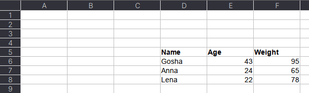
Чтобы прочитать такую таблицу, нужно указать диапазон в аргументе usecols. Также дополнительно можно добавить header — номер заголовка таблицы, а также nrows — количество строк, которые нужно прочитать. В аргументе header всегда передается номер строки на единицу меньше, чем в Excel-файле, поскольку в Python индексация начинается с 0 (на рисунке это номер 5, тогда указываем 4):
pd.read_excel(io='temp1.xlsx',
engine='openpyxl',
usecols='D:F',
header=4, # в excel это №5
nrows=3)
#
Name Age Weight
0 Gosha 43 95
1 Anna 24 65
2 Lena 22 78
Читаем таблицы в OpenPyXL
Pandas прочитывает только содержимое таблицы, но игнорирует метаданные: цвет заливки ячеек, примечания, стили таблицы и т.д. В таком случае пригодится библиотека OpenPyXL. Загрузка файлов осуществляется через функцию load_workbook, а к листам обращаться можно через квадратные скобки:
from openpyxl import load_workbook
wb = load_workbook('temp2.xlsx')
ws = wb['Лист1']
type(ws)
# openpyxl.worksheet.worksheet.Worksheet
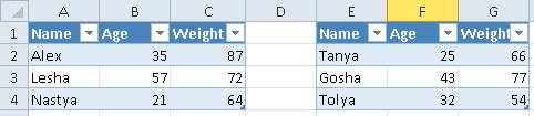
Допустим, имеется Excel-файл с несколькими таблицами на листе (см. рисунок выше). Если бы мы использовали Pandas, то он бы выдал следующий результат:
pd.read_excel(io='temp2.xlsx',
engine='openpyxl')
#
Name Age Weight Unnamed: 3 Name.1 Age.1 Weight.1
0 Alex 35 87 NaN Tanya 25 66
1 Lesha 57 72 NaN Gosha 43 77
2 Nastya 21 64 NaN Tolya 32 54
Можно, конечно, заняться обработкой и привести таблицы в нормальный вид, а можно воспользоваться OpenPyXL, который хранит таблицу и его диапазон в словаре. Чтобы посмотреть этот словарь, нужно вызвать ws.tables.items. Вот так выглядит Python-код:
ws.tables.items()
wb = load_workbook('temp2.xlsx')
ws = wb['Лист1']
ws.tables.items()
#
[('Таблица1', 'A1:C4'), ('Таблица13', 'E1:G4')]
Обращаясь к каждому диапазону, можно проходить по каждой строке или столбцу, а внутри них – по каждой ячейке. Например, следующий код на Python таблицы объединяет строки в список, где первая строка уходит на заголовок, а затем преобразует их в DataFrame:
dfs = []
for table_name, value in ws.tables.items():
table = ws[value]
header, *body = [[cell.value for cell in row]
for row in table]
df = pd.DataFrame(body, columns=header)
dfs.append(df)
Если таблицы имеют одинаковые атрибуты, то их можно соединить в одну:
pd.concat(dfs)
#
Name Age Weight
0 Alex 35 87
1 Lesha 57 72
2 Nastya 21 64
0 Tanya 25 66
1 Gosha 43 77
2 Tolya 32 54
Сохраняем метаданные таблицы
Как указано в коде выше, у ячейки OpenPyXL есть атрибут value, который хранит ее значение. Помимо value, можно получить тип ячейки (data_type), цвет заливки (fill), примечание (comment) и др.
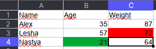
Например, требуется сохранить данные о цвете ячеек. Для этого мы каждую ячейку с числами перезапишем в виде <значение,RGB>, где RGB — значение цвета в формате RGB (red, green, blue). Python-код выглядит следующим образом:
# _TYPES = {int:'n', float:'n', str:'s', bool:'b'}
data = []
for row in ws.rows:
row_cells = []
for cell in row:
cell_value = cell.value
if cell.data_type == 'n':
cell_value = f"{cell_value},{cell.fill.fgColor.rgb}"
row_cells.append(cell_value)
data.append(row_cells)
Первым элементом списка является строка-заголовок, а все остальное уже значения таблицы:
pd.DataFrame(data[1:], columns=data[0])
#
Name Age Weight
0 Alex 35,00000000 87,00000000
1 Lesha 57,00000000 72,FFFF0000
2 Nastya 21,FF00A933 64,00000000
Теперь представим атрибуты в виде индексов с помощью метода stack, а после разобьём все записи на значение и цвет методом str.split:
(pd.DataFrame(data[1:], columns=data[0])
.set_index('Name')
.stack()
.str.split(',', expand=True)
)
#
0 1
Name
Alex Age 35 00000000
Weight 87 00000000
Lesha Age 57 00000000
Weight 72 FFFF0000
Nastya Age 21 FF00A933
Weight 64 0000000
Осталось только переименовать 0 и 1 на Value и Color, а также добавить атрибут Variable, который обозначит Вес и Возраст. Полный код на Python выглядит следующим образом:
(pd.DataFrame(data[1:], columns=data[0])
.set_index('Name')
.stack()
.str.split(',', expand=True)
.set_axis(['Value', 'Color'], axis=1)
.rename_axis(index=['Name', 'Variable'])
.reset_index()
)
#
Name Variable Value Color
0 Alex Age 35 00000000
1 Alex Weight 87 00000000
2 Lesha Age 57 00000000
3 Lesha Weight 72 FFFF0000
4 Nastya Age 21 FF00A933
5 Nastya Weight 64 00000000
Ещё больше подробностей о работе с таблицами в Pandas, а также их обработке на реальных примерах Data Science задач, вы узнаете на наших курсах по Python в лицензированном учебном центре обучения и повышения квалификации IT-специалистов в Москве.
Источники
- https://xlrd.readthedocs.io/en/latest/
- https://openpyxl.readthedocs.io/en/latest/
- https://github.com/eea/odfpy
- https://github.com/willtrnr/pyxlsb
Last updated on
Jul 18, 2021
In this post you can learn how to read Excel files (ext xls, xlsx etc) with Python and Pandas. We will import one or several sheets from an Excel file to a Pandas DataFrame.
The list of the supported file extensions:
xlsxlsxxlsmxlsbodfodsodt
Note for ods, ods and odt please check: Read Excel(OpenDocument ODS) with Python Pandas
Step 1: Install Pandas and odfpy
Python offers many different modules for reading and manipulating Excel files. In this guide we are going to use pandas and odfpy:
pip install pandas
pip install odfpy
Step 2: Read the one sheet of Excel(XLS) file
Pandas offers a powerful method for reading any type of Excel files read_excel(). It’s pretty easy to be used and requires only the file path:
import pandas as pd
pd.read_excel('animals.xls')
It will read and return all non empty cells from the Excel file:
| Rank | Animal | Maximum speed | Class | Notes | |
|---|---|---|---|---|---|
| 0 | 1 | Peregrine falcon | 389 km/h (242 mph)108 m/s (354 ft/s)[2][6] | Flight-diving | The peregrine falcon is the fastest aerial ani… |
| 1 | 2 | Golden eagle | 240–320 km/h (150–200 mph)67–89 m/s (220–293 f… | Flight-diving | Assuming the maximum size at 1.02 m, its relat… |
| 2 | 3 | White-throated needletail swift | 169 km/h (105 mph)[8][9][10] | Flight | NaN |
| 3 | 4 | Eurasian hobby | 160 km/h (100 mph)[11] | Flight | Can sometimes outfly the swift |
| 4 | 5 | Mexican free-tailed bat | 160 km/h (100 mph)[12] | Flight | It has been claimed to have the fastest horizo… |
| 5 | 6 | Frigatebird | 153 km/h (95 mph) | Flight | The frigatebird’s high speed is helped by its … |
| 6 | 7 | Rock dove (pigeon) | 148.9 km/h (92.5 mph)[13] | Flight | Pigeons have been clocked flying 92.5 mph (148… |
| 7 | 8 | Spur-winged goose | 142 km/h (88 mph)[14] | Flight | NaN |
| 8 | 9 | Gyrfalcon | 128 km/h (80 mph)[citation needed] | Flight | NaN |
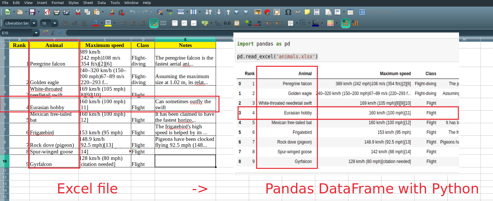
Step 3: Read the second sheet of Excel file by name
If you like to read data from a specific sheet — for example Sheet 2 then you can specify the name as a parameter — sheet_name:
pd.read_excel('animals.xlsx', sheet_name="Sheet2")
Which will result in:
| Blackbuck | Unnamed: 1 | |
|---|---|---|
| 0 | NaN | NaN |
| 1 | Male blackbuck | Male blackbuck |
| 2 | NaN | NaN |
| 3 | Female with young at the National Zoological Park Delhi | Female with young at the National Zoological P… |
| 4 | Conservation status | Conservation status |
| 5 | Least Concern (IUCN 3.1)[1] | Least Concern (IUCN 3.1)[1] |
| 6 | Scientific classification | Scientific classification |
Step 4: Python read excel file — specify columns and rows
If you like to read a range of data and not the whole sheet — read_excel offers several very useful parameters.
Python read excel file select rows
Next code example will show you how to read 3 rows skipping the first two rows. In this way Pandas will read only some rows from the whole sheet:
pd.read_excel('animals.xlsx', skiprows=2, nrows=3)
which will result in:
| 2 | Golden eagle | 240–320 km/h (150–200 mph)67–89 m/s (220–293 f… | Flight-diving | Assuming the maximum size at 1.02 m, its relat… | |
|---|---|---|---|---|---|
| 0 | 3 | White-throated needletail swift | 169 km/h (105 mph)[8][9][10] | Flight | NaN |
| 1 | 4 | Eurasian hobby | 160 km/h (100 mph)[11] | Flight | Can sometimes outfly the swift |
| 2 | 5 | Mexican free-tailed bat | 160 km/h (100 mph)[12] | Flight | It has been claimed to have the fastest horizo… |
Python read excel file select columns
If you like to** work with few columns** and not the whole sheet — then parameter use_cols can be used as shown:
pd.read_excel('animals.xlsx', usecols='C:D')
Python read excel file specify columns and rows
Finally if you like to select a range from specific columns and rows than you can use:
Which will result into:
| 240–320 km/h (150–200 mph)67–89 m/s (220–293 f… | Flight-diving | |
|---|---|---|
| 0 | 169 km/h (105 mph)[8][9][10] | Flight |
| 1 | 160 km/h (100 mph)[11] | Flight |
| 2 | 160 km/h (100 mph)[12] | Flight |
Step 5. Read multiple sheets from Excel file
What if you like to read with Pandas multiple sheets from Excel. It’s possible with pd.read_excel by providing a list of all sheets to be read as follows:
pd.read_excel('animals.xlsx', sheet_name=["Sheet1", "Sheet2"])
Note that a dictionary of
- keys — sheet names
- values — resulted DataFrames
will be returned.
In order to access data you can access it by a sheet name as:
pd.read_excel('animals.xlsx', sheet_name=["Sheet1", "Sheet2"]).get('Sheet1')
which will return the data for Sheet1 as a DataFrame.
Read All Sheets
For loading all sheets from Excel file use sheet_name=None:
pd.read_excel('animals.xlsx', sheet_name=None)
Step 6. Pandas read excel data with conversion, NA values and parsing
Finally let’s check what we can do if we need to convert data, drop or fill missing values, parse dates and numbers.
Pandas offers several parameters for this purpose:
- converters — dict of functions for converting values in certain columns
- keep_default_na — whether or not to include the default NaN values
- parse_dates
- ate_parser — converting a sequence of string columns to an array of datetime instances.
- thousands
- convert_float
You can check the Notebook in the resources for more examples of the above.
Resources
- Python Pandas Reading Excel files
- pandas.read_excel
- Notebook —
Read Excel ODS with Python Pandas
Мы можем использовать функцию read_excel() модуля pandas для чтения данных файла Excel в объекте DataFrame.
Если вы посмотрите на лист Excel, это двухмерная таблица. Объект DataFrame также представляет собой двумерную табличную структуру данных.
Содержание
- 1. Пример
- 2. Список заголовков столбцов таблицы Excel
- 3. Печать данных столбца
- 4. Пример использования команды read_excel()
- 5. Чтение файла без строки заголовка
- 6. Excel Sheet в Dict, CSV и JSON
1. Пример
Допустим, у нас есть файл Excel с двумя листами – «Employees» и «Cars». Верхняя строка содержит заголовок таблицы.

Вот пример для чтения данных таблицы «Employees» и их печати.
import pandas
excel_data_df = pandas.read_excel('records.xlsx', sheet_name='Employees')
# print whole sheet data
print(excel_data_df)
Вывод:
EmpID EmpName EmpRole 0 1 Pankaj CEO 1 2 David Lee Editor 2 3 Lisa Ray Author
- Первый параметр – это имя файла Excel.
- Параметр sheet_name определяет лист, который будет считан из файла Excel.
- Когда мы печатаем объект DataFrame, на выходе получается двумерная таблица. Это похоже на записи в Excel.
2. Список заголовков столбцов таблицы Excel
Мы можем получить список заголовков столбцов, используя свойство columns объекта dataframe.
print(excel_data_df.columns.ravel())
Вывод:
['EmpID' 'EmpName' 'EmpRole']
3. Печать данных столбца
Мы можем получить данные столбца и преобразовать их в список значений.
print(excel_data_df['EmpName'].tolist())
Вывод:
['Pankaj', 'David Lee', 'Lisa Ray']
Мы можем указать имена столбцов для чтения из файла Excel. Это полезно, когда вас интересуют только несколько столбцов таблицы Excel.
import pandas
excel_data_df = pandas.read_excel('records.xlsx', sheet_name='Cars', usecols=['Car Name', 'Car Price'])
print(excel_data_df)
Вывод:
Car Name Car Price 0 Honda City 20,000 USD 1 Bugatti Chiron 3 Million USD 2 Ferrari 458 2,30,000 USD
5. Чтение файла без строки заголовка
Если на листе Excel нет строки заголовка, передайте значение параметра заголовка как None.
excel_data_df = pandas.read_excel('records.xlsx', sheet_name='Numbers', header=None)
Если вы передадите значение заголовка как целое число, скажем, 3. Тогда третья строка будет рассматриваться как строка заголовка, и значения будут считываться со следующей строки. Все данные до строки заголовка будут отброшены.
6. Excel Sheet в Dict, CSV и JSON
Объект DataFrame имеет различные служебные методы для преобразования табличных данных в форматы Dict, CSV или JSON.
excel_data_df = pandas.read_excel('records.xlsx', sheet_name='Cars', usecols=['Car Name', 'Car Price'])
print('Excel Sheet to Dict:', excel_data_df.to_dict(orient='record'))
print('Excel Sheet to JSON:', excel_data_df.to_json(orient='records'))
print('Excel Sheet to CSV:n', excel_data_df.to_csv(index=False))
Вывод:
Excel Sheet to Dict: [{'Car Name': 'Honda City', 'Car Price': '20,000 USD'}, {'Car Name': 'Bugatti Chiron', 'Car Price': '3 Million USD'}, {'Car Name': 'Ferrari 458', 'Car Price': '2,30,000 USD'}]
Excel Sheet to JSON: [{"Car Name":"Honda City","Car Price":"20,000 USD"},{"Car Name":"Bugatti Chiron","Car Price":"3 Million USD"},{"Car Name":"Ferrari 458","Car Price":"2,30,000 USD"}]
Excel Sheet to CSV:
Car Name,Car Price
Honda City,"20,000 USD"
Bugatti Chiron,3 Million USD
Ferrari 458,"2,30,000 USD"
( 5 оценок, среднее 2 из 5 )