
What Is the Internal Rate of Return (IRR)?
The internal rate of return (IRR) is the discount rate providing a net value of zero for a future series of cash flows. Both the IRR and net present value (NPV) are used when selecting investments based on their returns.
Excel has three functions for calculating the internal rate of return that include Internal Rate of Return (IRR), Modified Internal Rate of Return (MIRR), and Internal Rate of Return with time periods (XIRR).
The IRR function calculates the internal rate of return for a series of cash flows, the MIRR function works with interest rates for borrowing and investing, and the XIRR function calculates a more accurate internal rate of return as it considers time periods.
Key Takeaways
• The internal rate of return (IRR) is the discount rate providing a net value of zero for a future series of cash flows.
• Excel has three functions for calculating the internal rate of return.
• When using different borrowing rates of reinvestment, a modified internal rate of return (MIRR) applies.
• The XIRR function accounts for different time periods.
How to Calculate IRR in Excel
What Is Net Present Value?
NPV is the difference between the present value of cash inflows and the present value of cash outflows over time.
The net present value of a project depends on the discount rate used. So when comparing two investment opportunities, the choice of the discount rate, which is often based on a degree of uncertainty, will have a considerable impact.
In the example below, using a 20% discount rate, investment #2 shows higher profitability than investment #1. When opting instead for a discount rate of 1%, investment #1 shows a return bigger than investment #2. Profitability often depends on the sequence and importance of the project’s cash flow and the discount rate applied to those cash flows.
How IRR and NPV Differ
The main difference between the IRR and NPV is that NPV is an actual amount while the IRR is the interest yield as a percentage expected from an investment.
Investors typically select projects with an IRR that is greater than the cost of capital. However, selecting projects based on maximizing the IRR as opposed to the NPV could result in suboptimal economic outcomes.
IRR represents the actual annual return on investment only when the project generates zero interim cash flows, or if those investments can be invested at the current IRR.
Calculating IRR in Excel
The IRR is the discount rate that can bring an investment’s NPV to zero. When the IRR has only one value, this criterion becomes more interesting when comparing the profitability of different investments.
In our example, the IRR of investment #1 is 48% and, for investment #2, the IRR is 80%. This means that in the case of investment #1, with an investment of $2,000 in 2013, the investment will yield an annual return of 48%. In the case of investment #2, with an investment of $1,000 in 2013, the yield will bring an annual return of 80%.
If no parameters are entered, Excel starts testing IRR values differently for the entered series of cash flows and stops as soon as a rate is selected that brings the NPV to zero. If Excel does not find any rate reducing the NPV to zero, it shows the error «#NUM.»
If the second parameter is not used and the investment has multiple IRR values, we will not notice because Excel will only display the first rate it finds that brings the NPV to zero.
In the image below, for investment #1, Excel does not find the NPV rate reduced to zero, so we have no IRR.
The image below also shows investment #2. If the second parameter is not used in the function, Excel will find an IRR of -10%. On the other hand, if the second parameter is used (i.e., = IRR ($ C $ 6: $ F $ 6, C12)), there are two IRRs rendered for this investment, which are -10% and 216%.
If the cash flow sequence has only a single cash component with one sign change (from + to — or — to +), the investment will have a unique IRR. However, most investments begin with a negative flow and a series of positive flows as the first investments come in. Profits then, hopefully, subside, as was the case in our first example.
In the image below, we calculate the IRR. To do this, we simply use the Excel IRR function:
Calculating MIRR in Excel
When a company uses different borrowing rates of reinvestment, the modified internal rate of return (MIRR) applies.
In the image below, we calculate the IRR of the investment as in the previous example but taking into account that the company will borrow money to plow back into the investment (negative cash flows) at a rate different from the rate at which it will reinvest the money earned (positive cash flow). The range C5 to E5 represents the investment’s cash flow range, and cells D10 and D11 represent the rate on corporate bonds and the rate on investments.
The image below shows the formula behind the Excel MIRR. We calculate the MIRR found in the previous example with the MIRR as its actual definition. This yields the same result: 56.98%.
(
−
NPV
(
rrate, values
[
positive
]
)
×
(
1
+
rrate
)
n
NPV
(
frate, values
[
negative
]
)
×
(
1
+
frate
)
)
1
n
−
1
−
1
begin{aligned}left(frac{-text{NPV}(textit{rrate, values}[textit{positive}])times(1+textit{rrate})^n}{text{NPV}(textit{frate, values}[textit{negative}])times(1+textit{frate})}right)^{frac{1}{n-1}}-1end{aligned}
(NPV(frate, values[negative])×(1+frate)−NPV(rrate, values[positive])×(1+rrate)n)n−11−1
Calculating XIRR in Excel
The XIRR function takes into consideration different periods. To use this function, Excel requires both the cash flow amounts as well as the dates on which those cash flows are paid.
In the example below, the cash flows are not disbursed at the same time each year – as is the case in the above examples. Rather, they are happening at different periods. We use the XIRR function below to solve this calculation. We first select the cash flow range (C5 to E5) and then select the range of dates on which the cash flows are realized (C32 to E32).
For investments with cash flows received or cashed at different moments in time for a firm that has different borrowing rates and reinvestments, Excel does not provide functions that can be applied to these situations although they are probably more likely to occur.
Excel for Microsoft 365 Excel for Microsoft 365 for Mac Excel for the web Excel 2021 Excel 2021 for Mac Excel 2019 Excel 2019 for Mac Excel 2016 Excel 2016 for Mac Excel 2013 Excel 2010 Excel 2007 Excel for Mac 2011 Excel Starter 2010 More…Less
This article describes the formula syntax and usage of the XIRR function in Microsoft Excel.
Description
Returns the internal rate of return for a schedule of cash flows that is not necessarily periodic. To calculate the internal rate of return for a series of periodic cash flows, use the IRR function.
Syntax
XIRR(values, dates, [guess])
The XIRR function syntax has the following arguments:
-
Values Required. A series of cash flows that corresponds to a schedule of payments in dates. The first payment is optional and corresponds to a cost or payment that occurs at the beginning of the investment. If the first value is a cost or payment, it must be a negative value. All succeeding payments are discounted based on a 365-day year. The series of values must contain at least one positive and one negative value.
-
Dates Required. A schedule of payment dates that corresponds to the cash flow payments. Dates may occur in any order. Dates should be entered by using the DATE function, or as results of other formulas or functions. For example, use DATE(2008,5,23) for the 23rd day of May, 2008. Problems can occur if dates are entered as text. .
-
Guess Optional. A number that you guess is close to the result of XIRR.
Remarks
-
Microsoft Excel stores dates as sequential serial numbers so they can be used in calculations. By default, January 1, 1900 is serial number 1, and January 1, 2008 is serial number 39448 because it is 39,448 days after January 1, 1900.
-
Numbers in dates are truncated to integers.
-
XIRR expects at least one positive cash flow and one negative cash flow; otherwise, XIRR returns the #NUM! error value.
-
If any number in dates is not a valid date, XIRR returns the #VALUE! error value.
-
If any number in dates precedes the starting date, XIRR returns the #NUM! error value.
-
If values and dates contain a different number of values, XIRR returns the #NUM! error value.
-
In most cases you do not need to provide guess for the XIRR calculation. If omitted, guess is assumed to be 0.1 (10 percent).
-
XIRR is closely related to XNPV, the net present value function. The rate of return calculated by XIRR is the interest rate corresponding to XNPV = 0.
-
Excel uses an iterative technique for calculating XIRR. Using a changing rate (starting with guess), XIRR cycles through the calculation until the result is accurate within 0.000001 percent. If XIRR can’t find a result that works after 100 tries, the #NUM! error value is returned. The rate is changed until:

where:
-
di = the ith, or last, payment date.
-
d1 = the 0th payment date.
-
Pi = the ith, or last, payment.
-
Example
Copy the example data in the following table, and paste it in cell A1 of a new Excel worksheet. For formulas to show results, select them, press F2, and then press Enter. If you need to, you can adjust the column widths to see all the data.
|
Data |
||
|
Values |
Dates |
|
|
-10,000 |
1-Jan-08 |
|
|
2,750 |
1-Mar-08 |
|
|
4,250 |
30-Oct-08 |
|
|
3,250 |
15-Feb-09 |
|
|
2,750 |
1-Apr-09 |
|
|
Formula |
Description (Result) |
Result |
|
=XIRR(A3:A7, B3:B7, 0.1) |
The internal rate of return (0.373362535 or 37.34%) |
37.34% |
Need more help?
Q. I have prepared projections for a proposed project, and I want to calculate the internal rate of return. Instead of using Excel’s IRR function, should I use simple math formulas so others can follow my calculations?
A. Excel offers three functions for calculating the internal rate of return, and I recommend you use all three. The problem with using math to calculate the internal rate of return is that the necessary calculations are both complicated and time—consuming. Basically, a math—based solution involves calculating the net present value (NPV) for each cash flow amount (in a series of cash flows) using various guessed interest rates on a trial—and—error basis, and then those NPVs are added together. This process is repeated using various interest rates until you find/stumble upon the exact interest rate that produces NPV amounts that sum to zero. The interest rate that produces a zero—sum NPV is then declared the internal rate of return.
To simplify this process, Excel offers three functions for calculating the internal rate of return, each of which represents a better option than using the math—based formulas approach. These Excel functions are IRR, XIRR, and MIRR. Explanations and examples for these functions are presented below. You can download the example workbook at carltoncollins.com/irr.xlsx.
1. Excel’s IRR function. Excel’s IRR function calculates the internal rate of return for a series of cash flows, assuming equal-size payment periods. Using the example data shown above, the IRR formula would be =IRR(D2:D14,.1)*12, which yields an internal rate of return of 12.22%. However, because some months have 31 days while others have 30 or fewer, the monthly periods are not exactly the same length, therefore, the IRR will always return a slightly erroneous result when multiple monthly periods are involved.
2. Excel’s XIRR function. Excel’s XIRR function calculates a more accurate internal rate of return because it takes into consideration different-size time periods. To use this function, you must supply both the cash flow amounts as well as the specific dates in which those cash flows are paid. In the example pictured below left, the XIRR formula would be =XIRR(D2:D14,B2:B14,.1), which yields an internal rate of return of 12.97%.
3. Excel’s MIRR function. Excel’s MIRR function (modified internal rate of return) works similarly to the IRR function, except that it also considers the cost of borrowing the initial investment funds as well as compounded interest earned by reinvesting each cash flow. The MIRR function is flexible enough to accommodate separate interest rates for borrowing and investing cash. Because the MIRR function calculates compound interest on project earnings or cash shortfalls, the resulting internal rate of return is usually significantly different from the internal rate of return produced by the IRR or XIRR function. In the example at left, the MIRR formula would be =MIRR(D2:D14,D16,D17)*12, which yields an internal rate of return of 17.68%.
Note: Some CPAs maintain that the MIRR function’s results are less valid because a project’s cash flows are rarely fully reinvested. However, clever CPAs can compensate for partial investment levels simply by adjusting the interest rate according to the expected levels of reinvestment. For instance, if it is assumed that reinvested cash flows will earn 3.0%, but only half the cash flows are expected to be reinvested, then the CPA can use an interest rate of 1.5% (half of 3.0%) as the interest rate to compensate for the partial investment of cash flows.
Rather than worrying about which method produces the more accurate result, I believe the best approach is to include all three calculations (IRR, XIRR, and MIRR) so the financial reader can consider them all. A few comments about these calculations follow.
1. Negative and positive cash flow values required. All three functions require at least one negative and at least one positive cash flow to complete the calculation. The first number in the cash flow series is typically a negative number that is assumed to be the project’s initial investment.
2. Monthly versus annual yields. When calculating the IRR or MIRR of monthly cash flows, the results must be multiplied by 12 to produce an annual yield; however, the XIRR function automatically produces an annual result that does not need to be multiplied. When calculating the IRR, XIRR, or MIRR of annual cash flows, the results do not need to be multiplied. (Because the XIRR function includes date ranges, it annualizes the results automatically.)
3. Guess. The IRR and XIRR functions allow you to enter a guess as the beginning rate where the function starts calculating incrementally, up to 20 cycles for the IRR function and 100 cycles for the XIRR function, until an answer within 0.00001% is found. If an answer is not determined within the allotted number of cycles, then the #NUM! error message is returned.
4. The #NUM! error. If the IRR function returns a #NUM! error value or if the result is not close to what you expected, Excel’s help files suggest you try again with a different value for your guess.
5. If you don’t enter a guess. If you don’t enter a guess for the IRR or XIRR function, Excel assumes 0.1, or 10%, as the initial guess.
6. Dates. The dates you enter must be entered as date values, not text, for the XIRR function to accurately use those dates.
About the author
J. Carlton Collins (carlton@asaresearch.com) is a technology consultant, a CPE instructor, and a JofA contributing editor.
Note: Instructions for Microsoft Office in “Technology Q&A” refer to the 2007 through 2016 versions, unless otherwise specified.
Submit a question
Do you have technology questions for this column? Or, after reading an answer, do you have a better solution? Send them to jofatech@aicpa.org. We regret being unable to individually answer all submitted questions.

Are you ready to kick it up a notch?
In this article, we will calculate the average and geometric average return of a stock, using Excel.
Suppose you are interested in buying Apple stock. Your first task is to calculate the stock return of Apple in the last 2 years.
First, we are going to obtain stock prices.
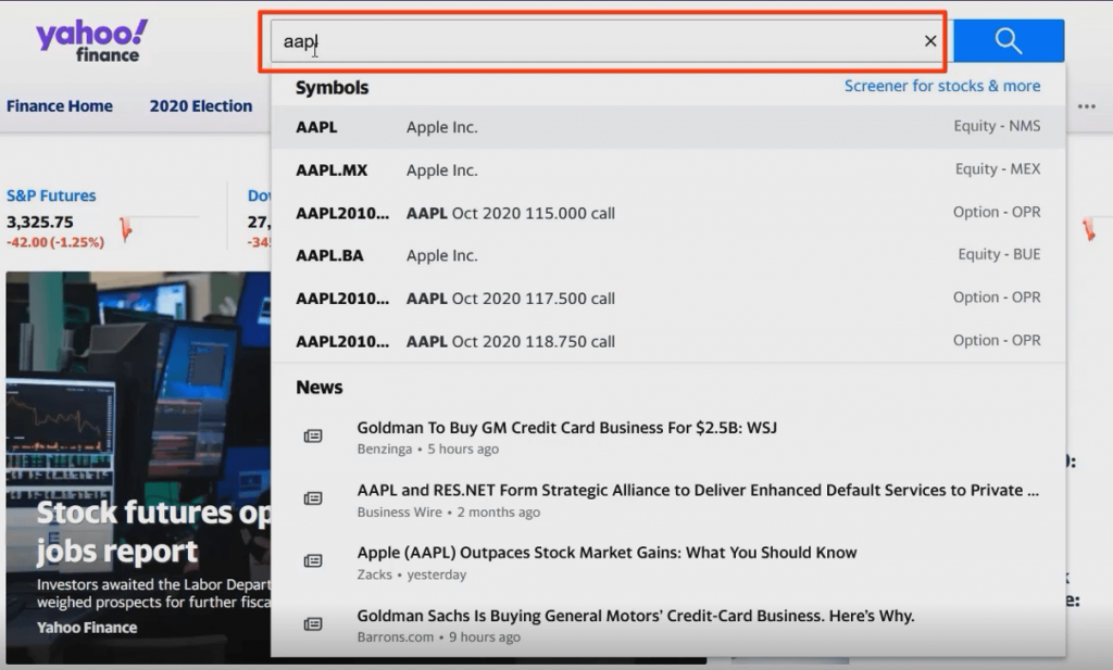
For this, we will use Yahoo Finance. We already know a thing or two about it, right?
We begin by typing the stock ticker. Do you remember what it is? “AAPL”!
Afterward, we select historical data. We download the stock prices over the last 2 years from July 1st, 2018 to July 1st, 2020.
Then, we need to set the data frequency.
There are 3 options to choose from – daily, weekly, or monthly.
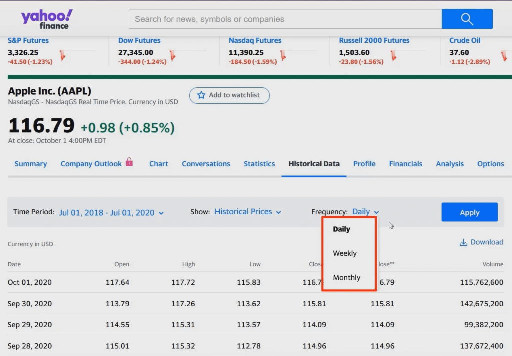
Basically, the choice of data frequency depends on the return you want to calculate.
When you estimate daily returns, you go for daily frequency. Weekly returns require weekly frequency. And so on.
Let’s say we are interested in calculating monthly returns. This gives us 24 data points.
We press ‘apply’ and then ‘download’, in order to retrieve the needed numbers.
Time to check out what we’ve got…
We open the downloaded file and come across the date and a whole bunch of information about the stock price, such as the opening, as well as the highest and lowest value during the period we’ve specified earlier.
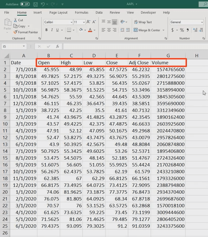
Which are the figures our calculations require, though?
Well, we want to use either the close or the adjusted close price. The former corrects for splits, whereas the adjusted one does so for both dividends AND splits.
Hence, we will use the adjusted close price. For conciseness, we get rid of all the information we won’t need and format the table in a more presentable way, based on the guidelines provided previously.
To save you some time, I have already done that.
Our next task is to calculate the holding period return for the stock.
What’s the formula we should be working with?
HPR = frac{Ending~value-Beginning~value}{Beginning~value}
It is the ending value of an investment minus its beginning value, divided by the beginning value.
In our example, we have $55.29 minus $46.22 divided by $46.22 which gives us approximately 19.6%.
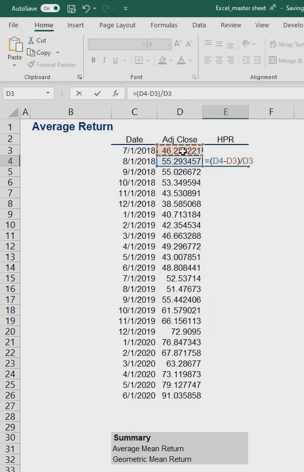
Finally, we go ahead and drag this formula all the way down.
Don’t forget to convert the values to percentages. Actually, you can get away with a simple shortcut.
Magicians never reveal their secrets, but we will willingly tell you ours: Excel is all about shortcuts! Be smart and use them as much as possible! This can save you a lot of time that you will eventually need for analyzing your data.
Here is one shortcut we can opt for, at this stage. Select the range of values, and then press and hold control plus shift, plus 5.
The last piece of the puzzle is to estimate the simple and geometric mean.
To obtain the former, we use the average function of Excel. We select the first argument and, after that, drag the range down to the last term.
Alternatively, we can use another useful shortcut. Press and hold Control plus shift plus the down arrow. This function marks the entire row of values below the cell you initially selected.
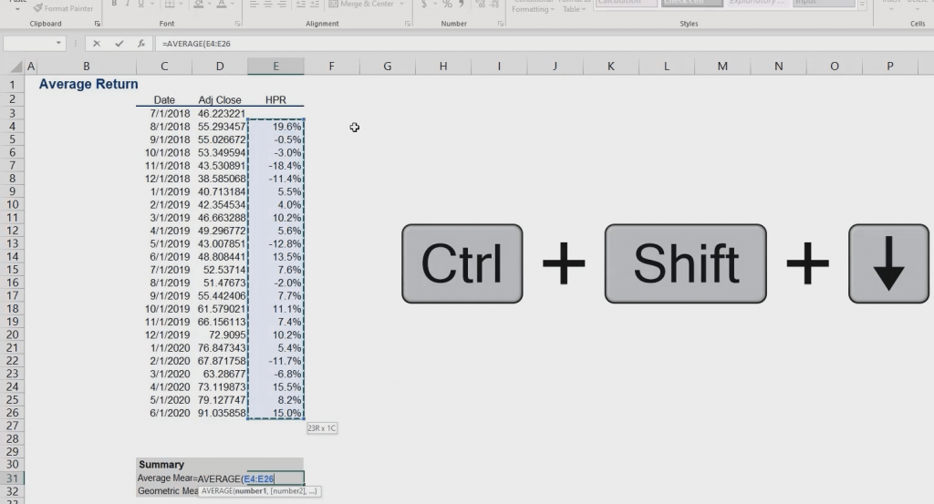
So, we estimate the mean return to be 3.49%.
Now, let’s calculate the geometric mean return.
For this purpose, we will use the geometric function. Basically, it gives us the geometric mean of an array or a range of positive data.
We type “GEOMEAN” and we pick the data range we will use. Don’t forget to add 1 to the expression before closing the parentheses.
The last step is to subtract 1 from the total.
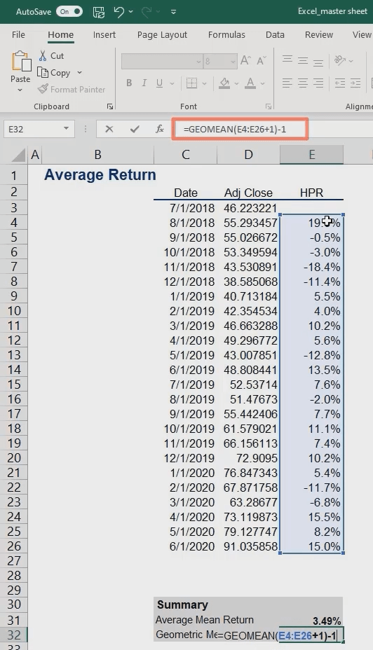
Excel interprets the expression in the following way: Add one to each of the returns and then take the geometric mean.
For those of you using earlier versions of Excel (2016 or older), you need to press Control, Shift and Enter after you key in the formula. This command makes Excel convert the expression to an array formula. In other words, it performs multiple calculations on one or more items in an array. If you have done that right, you will see braces that are added to the formula.
The geometric mean comes to 2.99%.
In our next article, we will learn how to measure the standard deviation of the stock’s returns.
Keep calm and invest on!

Ivan Kitov
We Think You Will Also Like
Rate of Return Formula (Table of Contents)
- Rate of Return Formula
- Rate of Return Calculator
- Rate of Return Formula in Excel (With Excel Template)
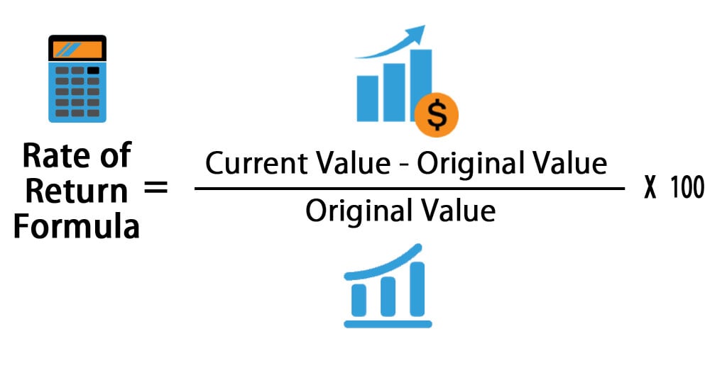
Rate of Return Formula
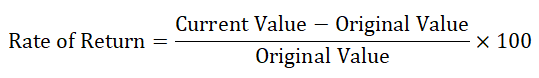
The Rate of return is return on investment over a period it could be profit or loss. It is basically a percentage of the amount above or below the investment amount. If the return of investment is positive that means there is a gain over investment and if the return of investment is negative that means there is a loss over investment. The rate of return is compared with gain or loss over investment. The rate of return expressed in form of percentage and also known as ROR. The rate of return formula is equal to current value minus original value divided by original value multiply by 100.
Here’s the Rate of Return formula –
Where,
- Current Value = Current value of investment.
- Original Value = Value of investment.
The rate of return over a time period of one year on investment is known as annual return.
Examples of Rate of Return Formula
Let us see an example to understand rate of return formula better.
You can download this Rate of Return Formula Excel Template here – Rate of Return Formula Excel Template
Rate of Return Formula – Example #1
An investor purchased a share at a price of $5 and he had purchased 1,000 shared in year 2017 after one year he decides to sell them at a price of $10 in the year 2018. Now, he wants to calculate the rate of return on his invested amount of $5,000.
As we know,
Rate of Return = (Current Value – Original Value) * 100 / Original Value
Put value in the above formula.
- Rate of Return = (10 * 1000 – 5 * 1000) * 100 / 5 *1000
- Rate of Return = (10,000 – 5,000) * 100 / 5,000
- Rate of Return = 5,000 * 100 / 5,000
- Rate of Return = 100%
Rate of return on shares is 100%.
Now, let’s see another example to understand the rate of return formula.
Rate of Return Formula – Example #2
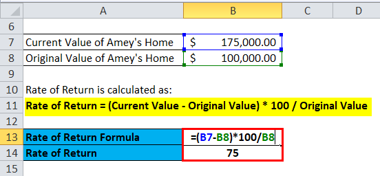
Amey had purchased home in year 2000 at price of $100,000 in outer area of city after sometimes area got develop, various offices, malls opened in that area which leads to an increase in market price of Amey’s home in the year 2018 due to his job transfer he has to sell his home at a price of $175,000. Now, let’s calculate the rate of return on his property.
As we know,
Rate of Return = (Current Value – Original Value) * 100 / Original Value
Put value in the above formula.
- Rate of Return = (175,000 – 100,000) * 100 / 100,000
- Rate of Return = 75,000 * 100 / 100,000
- Rate of Return = 75%
Rate of return on Amey’s home is 75%.
Annualize Rate of Return –
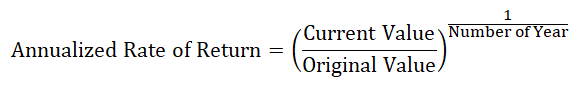
The regular rate of return tells about the gain or loss of an investment over a period of time. It is expressed in terms of percentage. The annualize rate on return also known as the Compound Annual Growth Rate (CAGR). It is return of investment every year. The annualized rate of return formula is equal to Current value upon original value raise to the power one divided by number of years, the whole component is then subtracted by one.
The formula for same can be written as:-
In this formula, any gain made is included in formula.
Let us see an example to understand it.
Rate of Return Formula – Example #3
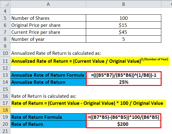
An investor purchase 100 shares at a price of $15 per share and he received a dividend of $2 per share every year and after 5 years sell them at a price of $45. Now, we have to calculate the annualized return for the investor.
As we know,
Annualized Rate of Return = (Current Value / Original Value)(1/Number of Year)
Put value in the formula.
- Annualized Rate of Return = (45 * 100 / 15 * 100)(1 /5 ) – 1
- Annualized Rate of Return = (4500 / 1500)0.2 – 1
- Annualized Rate of Return = 0.25
Hence,
Annualized Rate of Return = 25%
So, Annualize Rate of return on shares is 25%.
Now, let us calculate the rate of return on shares.
Rate of Return = (Current Value – Original Value) * 100 / Original Value
Put value in formula.
- Rate of Return = (45 * 100 – 15 * 100) * 100 / 15 * 100
- Rate of Return = (4500 – 1500) * 100 / 1500
- Rate of Return = 200%
Now, rate of return is 200% for shares.
Rate of return is also known as return on investment. The rate of return is applicable to all type of investments like stocks, real estate, bonds etc.
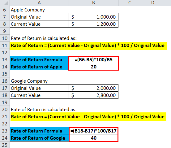
Rate of Return Formula – Example #4
Suppose an investor invests $1000 in shares of Apple Company in 2015 and sold his stock in 2016 at $1200.
Then, the rate of return will be:
- Rate of Return = (Current Value – Original Value) * 100 / Original Value
- Rate of Return Apple = (1200 – 1000) * 100 / 1000
- Rate of Return Apple = 200 * 100 / 1000
- Rate of Return Apple = 20%
He also invested $2000 in Google stocks in 2015 and sold his stock in 2016 at $2800.
Then the rate of return will be as follows:-
- Rate of Return = (Current Value – Original Value) * 100 / Original Value
- Rate of Return Google = (2800 – 2000) * 100 / 2000
- Rate of Return Google = 800 * 100 / 2000
- Rate of Return Google = 40%
So, through the rate of return, one can calculate the best investment option available. We can see that investor earns more profit in the investment of Google then in Apple, as the rate of return on investment in Google is higher than Apple.
Significance and Use of Rate of Return Formula
Rate of return have multiple uses they are as follows:-
- Rate of return is used in finance by corporates in any form of investment like assets, projects etc.
- Rate of return measure return on investment like rate of return on assets, rate of return on capital etc.
- Rate of return is useful in making investment decisions.
- It is used in financial analysis by investors.
Rate of Return Calculator
You can use the following Rate of Return Calculator
| Current Value | |
| Original Value | |
| Rate of Return Formula | |
| Rate of Return Formula = |
|
||||||||||
|
Rate of Return Formula in Excel (With Excel Template)
Here we will do the same example of the Rate of Return formula in Excel. It is very easy and simple. You need to provide the two inputs i.e Current Value and Original Value
You can easily calculate the Rate of Return using Formula in the template provided.
Example #1

Example #2
Example #3
Example #4
Conclusion
The rate of return is a popular metric because of its versatility and simplicity and can be used for any investment. Return of return is basically used to calculate the rate of return on investment and help to measure investment profitability. If the investment rate of return is positive then it’s probably worthwhile whereas if the rate of return is negative then it implies loss and hence investor should avoid it. The higher the percentage greater the benefit earned. One thing to keep in mind is considering the time value of money. For simple purchase or sale of stock the time value of money doesn’t matter, but for calculation of fixed asset like building, home where value appreciates with time. So, the annualized rate of return formula is used. One can use rate of return to compare performance rates on capital equipment purchase while an investor can calculate which stock purchases performed better
Recommended Articles
This has been a guide to a Rate of Return formula. Here we discuss its uses along with practical examples. We also provide you with Rate of Return Calculator with downloadable excel template. You may also look at the following articles to learn more –
- Debt to Income Formula
- Formula for Capital Gains Yield
- Guide to Bid-Ask Spread Formula
- Formula for Capacity Utilization Rate
- Annual Return Formula | How to Calculate? | Example