
Excel for Microsoft 365 Excel for Microsoft 365 for Mac Excel for the web Excel 2021 Excel 2021 for Mac Excel 2019 Excel 2019 for Mac Excel 2016 Excel 2016 for Mac Excel 2013 Excel 2010 Excel 2007 Excel for Mac 2011 Excel Starter 2010 More…Less
This article describes the formula syntax and usage of the RATE function in Microsoft Excel.
Description
Returns the interest rate per period of an annuity. RATE is calculated by iteration and can have zero or more solutions. If the successive results of RATE do not converge to within 0.0000001 after 20 iterations, RATE returns the #NUM! error value.
Syntax
RATE(nper, pmt, pv, [fv], [type], [guess])
Note: For a complete description of the arguments nper, pmt, pv, fv, and type, see PV.
The RATE function syntax has the following arguments:
-
Nper Required. The total number of payment periods in an annuity.
-
Pmt Required. The payment made each period and cannot change over the life of the annuity. Typically, pmt includes principal and interest but no other fees or taxes. If pmt is omitted, you must include the fv argument.
-
Pv Required. The present value — the total amount that a series of future payments is worth now.
-
Fv Optional. The future value, or a cash balance you want to attain after the last payment is made. If fv is omitted, it is assumed to be 0 (the future value of a loan, for example, is 0). If fv is omitted, you must include the pmt argument.
-
Type Optional. The number 0 or 1 and indicates when payments are due.
|
Set type equal to |
If payments are due |
|
0 or omitted |
At the end of the period |
|
1 |
At the beginning of the period |
-
Guess Optional. Your guess for what the rate will be.
-
If you omit guess, it is assumed to be 10 percent.
-
If RATE does not converge, try different values for guess. RATE usually converges if guess is between 0 and 1.
-
Remarks
Make sure that you are consistent about the units you use for specifying guess and nper. If you make monthly payments on a four-year loan at 12 percent annual interest, use 12%/12 for guess and 4*12 for nper. If you make annual payments on the same loan, use 12% for guess and 4 for nper.
Example
Copy the example data in the following table, and paste it in cell A1 of a new Excel worksheet. For formulas to show results, select them, press F2, and then press Enter. If you need to, you can adjust the column widths to see all the data.
|
Data |
Description |
|
|
4 |
Years of the loan |
|
|
-200 |
Monthly payment |
|
|
8000 |
Amount of the loan |
|
|
Formula |
Description |
Result |
|
=RATE(A2*12, A3, A4) |
Monthly rate of the loan with the terms entered as arguments in A2:A4. |
1% |
|
=RATE(A2*12, A3, A4)*12 |
Annual rate of the loan with the same terms. |
9.24% |
Need more help?
Want more options?
Explore subscription benefits, browse training courses, learn how to secure your device, and more.
Communities help you ask and answer questions, give feedback, and hear from experts with rich knowledge.
The RATE function in Excel is used to calculate the rate levied on a period of a loan. It is a built-in function in Excel. It takes the number of payment periods, pmt, present value, and future value as an input. The input provided to this formula is in integers, and the output is in percentages.
For example, suppose we have a dataset of the 5-year loan of $25,000 in cell B1 with monthly payments of $1000 in cell B2 has 60 periods in cell B3. We need to find the interest rate on the student loan. In such a scenario, we can use the RATE function in Excel:
=RATE(B3,B2,-B1)*12
=4.1%.
Table of contents
- RATE Excel Function
- RATE Formula in Excel
- Explanation
- How to Use RATE Function in Excel?
- Example #1
- Example #2
- Example #3
- Example #4
- Things to Remember
- Recommended Articles
RATE Formula in Excel

Explanation
Compulsory Parameter:
- Nper: Nper is the total number of the period for the loan/investment amount to be paid. For example, considering the 5 years terms means 5*12=60.
- Pmt: The fixed amount paid per period cannot be changed during the annuity’s life.
- Pv: Pv is the total loan amount or present value.
Optional Parameter:
- [Fv]: It is also called the future value and is optional in the RATE function in Excel. And if not passed in this function, it will be considered zero.
- [Type]: It can be omitted from the RATE function in Excel and used as 1 if payments are due at the beginning of the period and considered as 0 in case the payments are due at the end of the period.
- [Guess]: It is also an optional parameter; if omitted, it is assumed as 10%.
How to Use the RATE Function in Excel?
The RATE function in Excel is very simple and easy to use and can be used as a worksheet function and VBA function. Therefore, this function is used as a worksheet function.
You can download this Rate Function Excel Template here – Rate Function Excel Template
Example #1
Suppose the investment amount is 25,000, and the period is 5 years. Here the number of payments nperNPER, commonly known as the number of payment periods for a loan, is a financial term and an inbuilt financial function in Excel that can be used to calculate NPER for any loan. This formula takes rate, payment made, present value and future value as input from a user.read more will be =5*12=60 payments in total, and we have considered 500 as a fixed monthly payment and then calculated the interest rate using the RATE function in Excel.

Output will be: =RATE (C5, C4,-C3)*12 = 7.4%
Example #2
Let us consider another example wherein the interest rate per payment period on a 5,000 investment amount where monthly payments of 250 are made for 2 years so period will be=12*2=24. Here we have considered that all payments are made at the beginning of the period, so the type will be 1.
Calculation of interest rate are as follows:
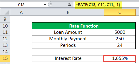
=RATE(C13,-C12, C11,, 1) output will be: 1.655%
Example #3
Let us take another example for weekly payment. This next example returns the interest rate on a loan amount of 8,000 where weekly payments of 700 are made for 4 years. Here, we have considered that all payments are made at the end of the period so that type will be 0 here.

The output will be: =RATE(C20,-C19, C18,, 0) = 8.750%.
Example #4
In the final example, we have considered that the loan amount will be 8,000, and annual payments of 950 are made for 10 years. Here, we assume that all the payments are made at the end of the period, then the type will be 0.
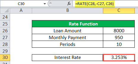
The output will be: =RATE(C28,-C27, C26) =3.253%
RATE in Excel is used as a VBA functionVBA functions serve the primary purpose to carry out specific calculations and to return a value. Therefore, in VBA, we use syntax to specify the parameters and data type while defining the function. Such functions are called user-defined functions.read more.
Dim Rate_value As Double
Rate_value = Rate(10*1, -950, 800)
Msgbox Rate_value
And output will be 0.3253
Things to Remember
Below are the few error details that can come in RATE in Excel if wrong arguments are passed in the RATE function in Excel.
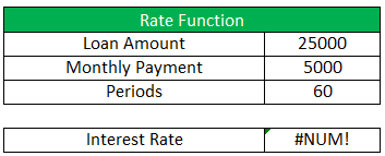
- Error handling #NUM!: If the interest RATE does not converge to 0.0000001 after 20 iterations, then the RATE excel function returns the #NUM! Error value.
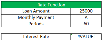
- Error handling #VALUE!: The RATE Excel function through a #VALUE! Error when any non-numeric value has been passed in the RATE formula in the Excel argument.
- We must convert the number of periods to month or quarter per your requirement.
- If the output of this function seems like 0, then there is no decimal value, then we must format the cell value to percentage format.
Recommended Articles
This article is a guide to Rate Function in Excel. Here, we discuss the RATE formula in Excel and how to use the RATE function, along with Excel examples and downloadable Excel templates. You may also look at these useful functions in Excel: –
- Negative Interest Rate MeaningWhen the interest rate falls below 0 percent, we have a negative interest scenario. This implies that banks will charge you interest for keeping your money with them. It is more common during periods of extreme deflation.read more
- Excel Record MacrosRecording macros is a method whereby excel stores the tasks performed by the user. Every time a macro is run, these exact actions are performed automatically. Macros are created in either the View tab (under the “macros” drop-down) or the Developer tab of Excel.
read more - MODE Excel Function
- MONTH Excel FunctionThe Month Function is a date function that determines the month for a given date in date format. It takes an argument in a date format and displays the result in integer format.read more
- Insert (Embed) an Object in ExcelIn Microsoft Excel, the “Object Insert” option allows a user to insert an external object into a worksheet. Embedding generally means inserting an object from another software (Word, PDF, etc.) into an Excel worksheet.read more
- Функция RATE в Excel

Функция RATE (Содержание)
- Функция RATE в Excel
- RATE Формула в Excel
- Как использовать функцию RATE?
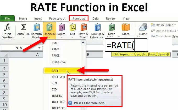
Функция RATE в Excel
Давайте возьмем пример. Рам хочет взять кредит / занять немного денег или хочет вложить деньги в финансовую компанию XYZ. Компания должна сделать некоторые финансовые расчеты, например, клиент должен заплатить что-то финансовому предприятию в счет суммы кредита или того, сколько клиенту нужно инвестировать, чтобы через некоторое время он / она мог получить такую большую сумму денег.
В этих сценариях Excel имеет наиболее важную функцию «СКОРОСТЬ», которая является частью финансовой функции.
Что такое функция RATE?
Функция, которая используется для расчета процентной ставки для оплаты указанной суммы кредита или для получения указанной суммы инвестиций через некоторый период времени, называется функцией RATE.
RATE Formula
Ниже приведена формула RATE:
Функция RATE использует ниже аргументы
Nper: Всего нет. периодов для займа или инвестиций.
Pmt: платеж производится каждый период, и это фиксированная сумма во время кредита или инвестиций.
Pv: текущая (текущая) стоимость кредита / инвестиции.
(Fv): это необязательный аргумент. Это указывает будущую стоимость кредита / инвестиций в конце общего нет. платежей (nper) платежей.
Если не указать какое-либо значение, оно автоматически считает fv = 0.
(тип): это также необязательный аргумент. Он принимает логические значения 0 или 1.
1 = если оплата произведена в начале периода.
0 = если оплата произведена в конце периода.
Если не указать какое-либо значение, оно автоматически считает его равным 0.
(предположение): первоначальное предположение о том, какой будет ставка. Если не указать какое-либо значение, оно автоматически считает это 0, 1 (10%).
Объяснение функции RATE:
Функция RATE используется в разных сценариях.
- PMT (оплата)
- PV (текущая стоимость)
- FV (будущая стоимость)
- NPER (количество периодов)
- IPMT (выплата процентов)
Как использовать функцию RATE в Excel?
Функция RATE очень проста в использовании. Давайте теперь посмотрим, как использовать функцию RATE в Excel с помощью нескольких примеров.
Вы можете скачать этот шаблон функции RATE здесь — шаблон функции RATE
Пример № 1
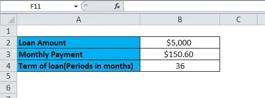
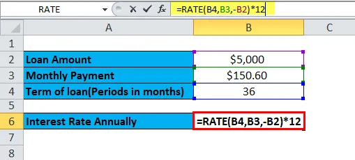
Вы хотите купить машину. Для этого вы подаете заявку в банк на 5000 долларов. Банк предоставляет этот кредит сроком на 5 лет и фиксирует сумму ежемесячного платежа в размере 150, 60 долларов США. Теперь вам нужно знать годовую процентную ставку.
Здесь у нас есть следующая информация:
= СКОРОСТЬ (B4, B3, -B2)
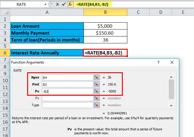
Здесь результат функции умножается на 12, дает годовую процентную ставку. B2 — отрицательное значение, потому что это исходящий платеж.
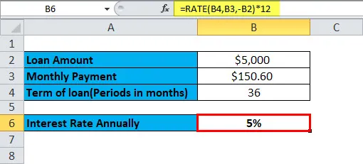
= СКОРОСТЬ (B4, B3, -B2) * 12
Годовая процентная ставка будет:
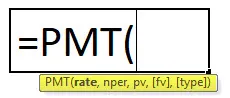
PMT (оплата)
Эта функция используется для расчета платежей, осуществляемых каждый месяц по кредиту или инвестициям, на основе фиксированного платежа и постоянной процентной ставки.
PMT Формула:
Пример № 2
Вы хотите купить дом, который стоит 350 000 долларов. Чтобы купить это, вы хотите подать заявку на банковский кредит. Банк предлагает вам кредит под 18% годовых на 10 лет. Теперь вам нужно рассчитать ежемесячный взнос или оплату этого кредита.
Здесь у нас есть следующая информация:
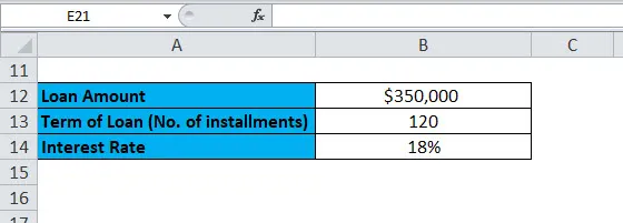
Процентная ставка дается ежегодно, следовательно, делится на 12, чтобы конвертировать в ежемесячную процентную ставку.
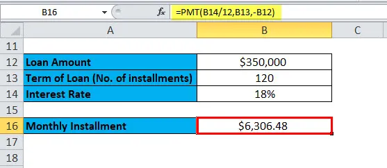
= PMT (B14 / 12, B13, -B12)
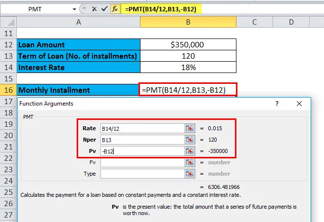
Результатом будет:
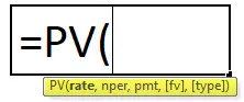
PV (текущая стоимость)
Эта функция рассчитывает текущую стоимость инвестиций или кредита, взятых по фиксированной процентной ставке. Или, другими словами, он рассчитывает текущую стоимость с постоянными выплатами, или будущую стоимость, или инвестиционную цель.
Формула PV:
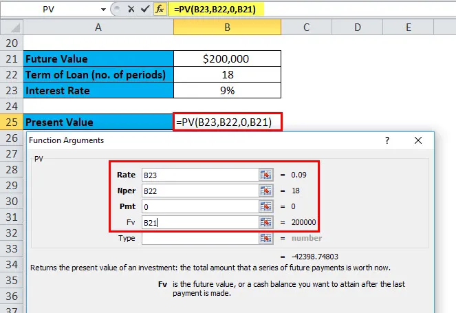
Пример № 3
Вы сделали инвестицию, которая выплачивает вам 200 000 долларов через 18 лет под 9% годовых. Теперь вам нужно узнать, сколько нужно инвестировать сегодня, чтобы вы могли получить будущую стоимость в 200 000 долларов.
Здесь у нас есть следующая информация:
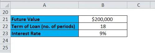
= PV (B23, B22, 0, B21)
Результат:
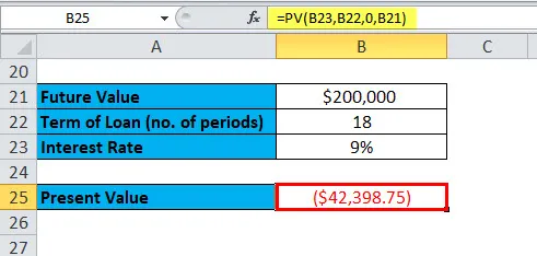
Результат в отрицательных числах, так как это денежный приток или входящие платежи.
Давайте возьмем еще один пример функции PV.
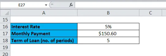
Пример № 4
Вы взяли кредит на 5 лет с фиксированной суммой ежемесячного платежа в размере 150, 60 долларов США. Годовая процентная ставка составляет 5%. Теперь вам нужно рассчитать первоначальную сумму кредита.
Здесь у нас есть следующая информация:
= PV (5 / 12, 5 * 12, -B17, 0)
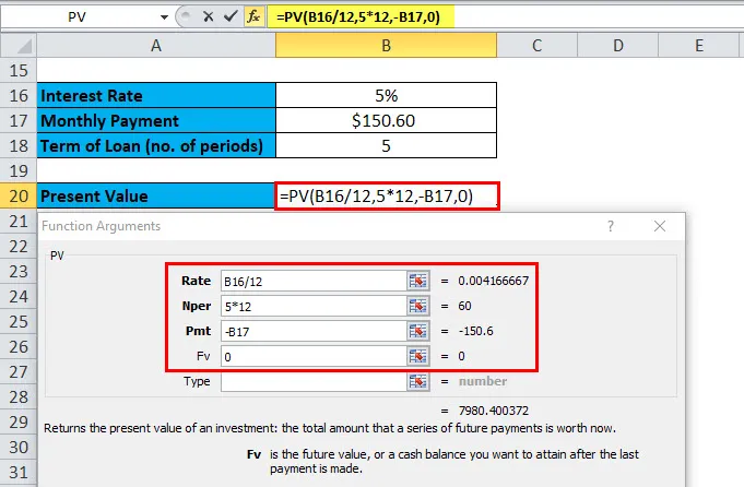
Результат:
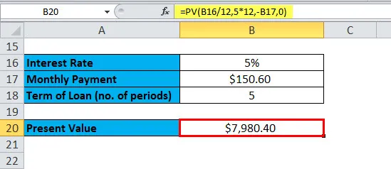
Этот ежемесячный платеж был округлен до ближайшей копейки.
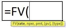
FV (будущая стоимость)
Эта функция используется для определения будущей стоимости инвестиций.
Формула FV:
Пример № 5
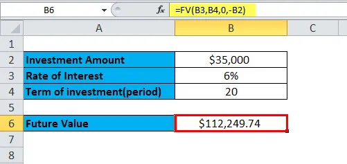
Вы вкладываете определенную сумму в размере 35 000 долларов США под 6% годовых в течение 20 лет. Теперь вопрос: с этими инвестициями, сколько мы получим через 20 лет?
Здесь у нас есть следующая информация:
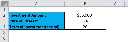
= FV (B3, B4, 0, -B2)
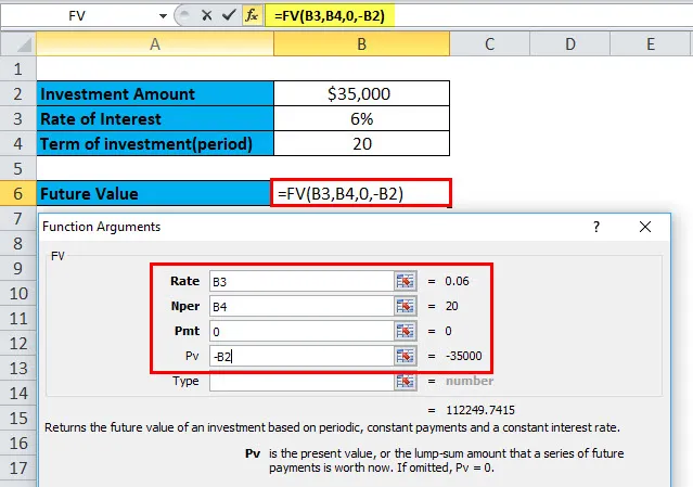
Результат:
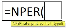
NPER (количество периодов)
Эта функция возвращает общее число. периодов для инвестиций или для кредита.
NPER Формула:
Пример № 6
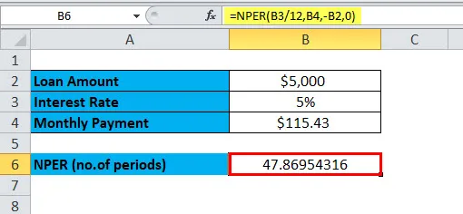
Вы берете кредит на сумму 5000 долларов США с ежемесячной суммой выплат в размере 115, 43 доллара США. Кредит имеет 5% годовых. Для расчета нет. периодов, нам нужно использовать функцию NPER.
Здесь у нас есть следующая информация:
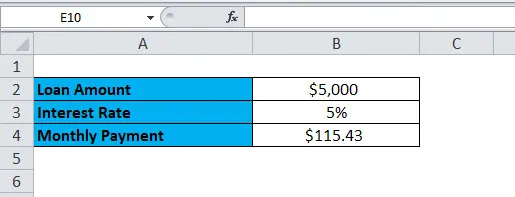
= NPER (B3 / 12, B4, -B2, 0)
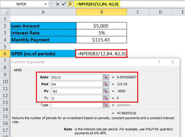
Эта функция возвращает 47, 869, т.е. 48 месяцев.
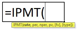
IPMT (выплата процентов)
Эта функция возвращает выплату процентов по кредиту или инвестициям за определенный период времени.
Формула IPMT
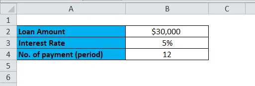
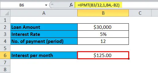
Пример № 7
Вы взяли кредит в размере 30 000 долларов США на один год с годовой процентной ставкой 5%. Теперь для расчета процентной ставки за первый месяц мы будем использовать функцию IPMT.
Здесь у нас есть следующая информация:
= ПРПЛТ (B3 / 12, 1, В4, ~В2)
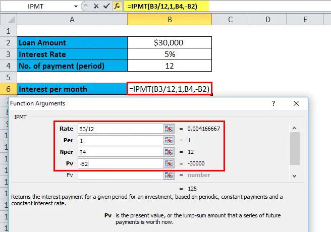
Результат:
Что нужно помнить о функции RATE
В индустрии финансов обычно используются два фактора: отток денежных средств и приток денежных средств.
Отток денежных средств: исходящие платежи обозначаются отрицательными числами.
Приток денежных средств: входящие платежи обозначаются положительными числами.
Рекомендуемые статьи
Это было руководство к функции Excel RATE. Здесь мы обсуждаем формулу RATE и как использовать функцию RATE вместе с практическими примерами и загружаемым шаблоном Excel. Вы также можете просмотреть наши другие предлагаемые статьи —
- Использование функции ИЛИ в MS Excel
- Использование функции NOT в MS Excel
- Использование функции AND в MS Excel
- Использование LOOKUP в MS Excel?
Purpose
Get the interest rate per period of an annuity
Return value
The interest rate per period
Usage notes
The RATE function returns the interest rate per period of an annuity. You can use RATE to calculate the periodic interest rate, then multiply as required to derive the annual interest rate. The RATE function calculates by iteration. If the results of RATE do not converge within 20 iterations, RATE returns the #NUM! error value.
The RATE function takes six separate arguments, three of which are required as explained below.
nper (required) — The total number of payment periods in the annuity. For example, a 5-year car loan with monthly payments has 60 periods. You can enter nper as 5*12 to show how the number was determined.
pmt (required) — The payment made each period. This number cannot change over the life of the annuity. In annuity functions, cash paid out is represented by a negative number. Note: If pmt is not provided, the optional fv argument must be supplied.
pv (optional) — The present value. This is the cash balance required after all payments have been made.
fv (optional) — The future value, or a cash balance required after the last payment is made. When fv is omitted, it defaults to zero (0) and pmt must be provided.
type (optional) — type is a boolean that controls when when payments are due. Use 0 for payments due at the end of the period (regular annuities) and 1 for payments due at the end of the period (annuities due). Type defaults to 0 (end of period).
guess (optional) — guess is a seed value to use for iteration. When omitted, guess defaults to 10%. Ordinarily, you can safely omit guess. If RATE does not converge, RATE will return a #NUM! error. Try different values for guess between 0 and 1.
Example
To calculate the annual interest rate for a $5000 loan with payments of $93.22 per month over 5 years, you can use RATE in a formula like this:
=RATE(60,-93.22,5000)*12 // returns 4.5%
In the example shown, the formula in C10 is:
=RATE(C7,-C6,C5)*C8 // returns 4.5%
Notice the value for pmt from C6 is entered as a negative value.
Notes
You must use consistent values for for guess and nper. If you make monthly payments on a five-year loan at 10 percent annual interest, use 10%/12 for guess and 5*12 for nper. If you make annual payments on the same loan, use 10% for guess and 5 for nper.