
Расширенный фильтр и немного магии
У подавляющего большинства пользователей Excel при слове «фильтрация данных» в голове всплывает только обычный классический фильтр с вкладки Данные — Фильтр (Data — Filter):

Такой фильтр — штука привычная, спору нет, и для большинства случаев вполне сойдет. Однако бывают ситуации, когда нужно проводить отбор по большому количеству сложных условий сразу по нескольким столбцам. Обычный фильтр тут не очень удобен и хочется чего-то помощнее. Таким инструментом может стать расширенный фильтр (advanced filter), особенно с небольшой «доработкой напильником» (по традиции).
Основа
Для начала вставьте над вашей таблицей с данными несколько пустых строк и скопируйте туда шапку таблицы — это будет диапазон с условиями (выделен для наглядности желтым):

Между желтыми ячейками и исходной таблицей обязательно должна быть хотя бы одна пустая строка.
Именно в желтые ячейки нужно ввести критерии (условия), по которым потом будет произведена фильтрация. Например, если нужно отобрать бананы в московский «Ашан» в III квартале, то условия будут выглядеть так:

Чтобы выполнить фильтрацию выделите любую ячейку диапазона с исходными данными, откройте вкладку Данные и нажмите кнопку Дополнительно (Data — Advanced). В открывшемся окне должен быть уже автоматически введен диапазон с данными и нам останется только указать диапазон условий, т.е. A1:I2:

Обратите внимание, что диапазон условий нельзя выделять «с запасом», т.е. нельзя выделять лишние пустые желтые строки, т.к. пустая ячейка в диапазоне условий воспринимается Excel как отсутствие критерия, а целая пустая строка — как просьба вывести все данные без разбора.
Переключатель Скопировать результат в другое место позволит фильтровать список не прямо тут же, на этом листе (как обычным фильтром), а выгрузить отобранные строки в другой диапазон, который тогда нужно будет указать в поле Поместить результат в диапазон. В данном случае мы эту функцию не используем, оставляем Фильтровать список на месте и жмем ОК. Отобранные строки отобразятся на листе:

Добавляем макрос
«Ну и где же тут удобство?» — спросите вы и будете правы. Мало того, что нужно руками вводить условия в желтые ячейки, так еще и открывать диалоговое окно, вводить туда диапазоны, жать ОК. Грустно, согласен! Но «все меняется, когда приходят они ©» — макросы!
Работу с расширенным фильтром можно в разы ускорить и упростить с помощью простого макроса, который будет автоматически запускать расширенный фильтр при вводе условий, т.е. изменении любой желтой ячейки. Щелкните правой кнопкой мыши по ярлычку текущего листа и выберите команду Исходный текст (Source Code). В открывшееся окно скопируйте и вставьте вот такой код:
Private Sub Worksheet_Change(ByVal Target As Range)
    If Not Intersect(Target, Range("A2:I5")) Is Nothing Then
        On Error Resume Next
        ActiveSheet.ShowAllData
        Range("A7").CurrentRegion.AdvancedFilter Action:=xlFilterInPlace, CriteriaRange:=Range("A1").CurrentRegion
    End If
End Sub
Эта процедура будет автоматически запускаться при изменении любой ячейки на текущем листе. Если адрес измененной ячейки попадает в желтый диапазон (A2:I5), то данный макрос снимает все фильтры (если они были) и заново применяет расширенный фильтр к таблице исходных данных, начинающейся с А7, т.е. все будет фильтроваться мгновенно, сразу после ввода очередного условия:

Так все гораздо лучше, правда? 
Реализация сложных запросов
Теперь, когда все фильтруется «на лету», можно немного углубиться в нюансы и разобрать механизмы более сложных запросов в расширенном фильтре. Помимо ввода точных совпадений, в диапазоне условий можно использовать различные символы подстановки (* и ?) и знаки математических неравенств для реализации приблизительного поиска. Регистр символов роли не играет. Для наглядности я свел все возможные варианты в таблицу:
| Критерий | Результат |
| гр* или гр | все ячейки начинающиеся с Гр, т.е. Груша, Грейпфрут, Гранат и т.д. |
| =лук | все ячейки именно и только со словом Лук, т.е. точное совпадение |
| *лив* или *лив | ячейки содержащие лив как подстроку, т.е. Оливки, Ливер, Залив и т.д. |
| =п*в | слова начинающиеся с П и заканчивающиеся на В т.е. Павлов, Петров и т.д. |
| а*с | слова начинающиеся с А и содержащие далее С, т.е. Апельсин, Ананас, Асаи и т.д. |
| =*с | слова оканчивающиеся на С |
| =???? | все ячейки с текстом из 4 символов (букв или цифр, включая пробелы) |
| =м??????н | все ячейки с текстом из 8 символов, начинающиеся на М и заканчивающиеся на Н, т.е. Мандарин, Мангостин и т.д. |
| =*н??а | все слова оканчивающиеся на А, где 4-я с конца буква Н, т.е. Брусника, Заноза и т.д. |
| >=э | все слова, начинающиеся с Э, Ю или Я |
| <>*о* | все слова, не содержащие букву О |
| <>*вич | все слова, кроме заканчивающихся на вич (например, фильтр женщин по отчеству) |
| = | все пустые ячейки |
| <> | все непустые ячейки |
| >=5000 | все ячейки со значением больше или равно 5000 |
| 5 или =5 | все ячейки со значением 5 |
| >=3/18/2013 | все ячейки с датой позже 18 марта 2013 (включительно) |
Тонкие моменты:
- Знак * подразумевает под собой любое количество любых символов, а ? — один любой символ.
- Логика в обработке текстовых и числовых запросов немного разная. Так, например, ячейка условия с числом 5 не означает поиск всех чисел, начинающихся с пяти, но ячейка условия с буквой Б равносильна Б*, т.е. будет искать любой текст, начинающийся с буквы Б.
- Если текстовый запрос не начинается со знака =, то в конце можно мысленно ставить *.
- Даты надо вводить в штатовском формате месяц-день-год и через дробь (даже если у вас русский Excel и региональные настройки).
Логические связки И-ИЛИ
Условия записанные в разных ячейках, но в одной строке — считаются связанными между собой логическим оператором И (AND):
Т.е. фильтруй мне бананы именно в третьем квартале, именно по Москве и при этом из «Ашана».
Если нужно связать условия логическим оператором ИЛИ (OR), то их надо просто вводить в разные строки. Например, если нам нужно найти все заказы менеджера Волиной по московским персикам и все заказы по луку в третьем квартале по Самаре, то это можно задать в диапазоне условий следующим образом:

Если же нужно наложить два или более условий на один столбец, то можно просто продублировать заголовок столбца в диапазоне критериев и вписать под него второе, третье и т.д. условия. Вот так, например, можно отобрать все сделки с марта по май:

В общем и целом, после «доработки напильником» из расширенного фильтра выходит вполне себе приличный инструмент, местами не хуже классического автофильтра.
Ссылки по теме
- Суперфильтр на макросах
- Что такое макросы, куда и как вставлять код макросов на Visual Basic
- Умные таблицы в Microsoft Excel
VBA Advanced Filter is one of the many hidden gems that Excel VBA offers to make our time more productive.
VBA Advanced Filter requires very little code, is one of the fastest ways to copy data, and provides advanced filtering options that we cannot get anywhere else.
VBA Advanced Filter Quick Guide
Using the criteria with AdvancedFilter is very powerful. You can see the possible options in the table below:
| Task | Cell formula | Examples where true |
|---|---|---|
| Contains | Pea =»Pea» =»*Pea*» |
Peach, Pea, Appear |
| Does not contain | =»<>*Pea*» | any text that does not contain Pea |
| Exact match | =»=Pea» | Pea |
| Does not exactly match | =»<>Pea» | Peach, Pear etc. |
| Starts with | =»=Pea*» | Peach, Pear, Pea |
| Ends with | =»=*Pea» | SweetPea, GreenPea |
| Use the ? symbol to represent any single character | =»=Pea?» | Pear, Peas or any 4 letter word starting with «Pea» |
| Any of the symbols *?~ | =»=Pea~*» | Pea*, Pea? |
| Case sensitive(see section Using Formulas as Criteria) | =EXACT(A7,»Peach») | Peach |
| Greater than | =»>700″ | 701,702 etc. |
| Greater than or equals | =»>=700″ | 700, 701,702 etc. |
| Less than | =»<700″ | 699,698 etc. |
| Less than or equals | =»<=700″ | 700, 699, 698 etc. |
| Equals | =»=700″ | 700 |
Important Note: A Criteria column header must exist as a List range column header. For example, if the Criteria column header is “Fruit” then there must be a List range column header called “Fruit”.
Here are some important things to know about the Criteria column headers:
- They can be used in any order.
- You can use the same header multiple times(see section Advanced Filter Multiple Criteria below).
- You don’t need to include a column header in the criteria if you are not filtering by this column.
What is Advanced Filter
Advanced Filter is a tool that is available in the Sort & Filter section of the Data tab on the Excel Ribbon:

It allows us to filter data based on a Criteria range. This allows us to do more advanced filtering than the standard filtering on the worksheet.
A second advantage of using Advanced Filter is that we have the option to copy the results to a new range if we choose.
Using Advanced Filter is quite simple as you can see from the dialog:

We filter in-place or we copy to another location. We then simply need the data range(List range) and the Criteria Range. If we decided to copy to another location then we provide the “Copy to” range.
Using Advanced Filter is very useful in VBA because it is extremely fast, powerful and as we will see it requires very little code.
VBA Advanced Filter on YouTube
To see me working with Advanced Filter, check out this YouTube video:
VBA Advanced Filter Parameters
The following table shows the parameters of the AdvancedFilter function:
| Parameter | Optional | Type | Details |
|---|---|---|---|
| Action | Required | xlFilterAction | xlFilterInPlace or xlFilterCopy. |
| CriteriaRange | Optional | Range | Range of the criteria used for filtering the data. |
| CopyToRange | Optional | Range | Destination range if Action is set to xlFilterCopy. |
| Unique | Optional | Boolean | True for unique records only. |
You can read about the parameters on the Microsoft help page.
AdvancedFilter requires three ranges to run(or two if you are using xlFilterInPlace as the Action parameter):
- List range – data to filter.
- Criteria range – how to filter.
- Copy To range – where to place the results if the Action parameter is set to xlFilterCopy is set.
AdvancedFilter is a range Function. This means you get the range of data you wish to filter and then call the AdvancedFilter function of that range:
DataRange.AdvancedFilter Filter Action, Criteria, [CopyTo], [Unique]
We can filter in place or we can copy the filter results to another location. This means there are two ways to use AdvancedFilter:
 ' Filter in place
 rgData.AdvancedFilter xlFilterInPlace, rgCriteriaRange

 ' Filter and copy data
 rgData.AdvancedFilter xlFilterCopy, rgCriteriaRange, rgDestination
The first parameter indicates the way to apply the filter:
- xlFilterInPlace – Filter the original data.
- xlFilterCopy – Copy the filter results to a new range.
If we use xlFilterInPlace then we don’t need the destination range.
To remove duplicate records we simply set the Unique parameter to True. Otherwise, duplicate records are ignored:
 ' Filter in place
 rgData.AdvancedFilter xlFilterInPlace, rgCriteriaRange, , True

 ' Filter and copy data
 rgData.AdvancedFilter xlFilterCopy, rgCriteriaRange, rgDestination, True
Understanding the Advanced Filter Ranges
The following screenshot shows an example of the 3 ranges. The List(or data) range is shaded blue, the Criteria range is green, and the CopyTo range is yellow:

The following subsection provides a quick guide to each of the ranges:
Criteria Range
- The criteria headers must be one of the List Range column headers. If not then it will be ignored.
- Criteria headers can be in any order.
- You can include as many or as few Criteria headers as you need.
- You can use the same header multiple times – this allows us to do multiple AND operations on the same column.
CopyTo Range
- This range is only used when the Action parameter is set to xlFilterCopy.
- To avoid errors this range should be the Header row of the output destination.
- You can use any(or all) columns from the List range as your output and they can be in any order.
- The columns headers in this range must be a List Range column header or you will get a VBA Runtime Error 1004.
List Range
- The List Range is the range of data that will be filtered.
- You must include the headers as part of the List Range.
- If you set the Action parameter to xlFilterInPlace then the List data will be filtered.
- If you set the Action parameter to xlFilterCopy then the results will be copied to the location which is specified in the CopyToRange parameter.
Writing the VBA Code
The easiest way to define the data range is to use CurrentRegion although you can get the range any way you like. Using CurrentRegion gets all the adjacent data to the specified cell or range.
We can use CurrentRegion like this:
 Dim rgData As Range, rgCriteriaRange As Range
 Set rgData = Range("A4").CurrentRegion
 Set rgCriteriaRange = Range("A1").CurrentRegion
To set the CopyTo range, you specify the entire heading row.
You can use a simple trick with CurrentRegion to get the CopyToRange header row. First, use CurrentRegion and then take the first row of the resulting range:
 Dim rgCopyToRange As Range
 Set rgCopyToRange = shFruit.Range("E4").CurrentRegion.Rows(1)
The full VBA Advanced filter code looks like this:
Sub RunAdvancedFilter()

    ' Declare the variables
    Dim rgData As Range, rgCriteriaRange As Range, rgCopyToRange As Range

    ' Set the ranges
    Set rgData = Sheet1.Range("A4").CurrentRegion
    Set rgCriteriaRange = Sheet1.Range("A1").CurrentRegion
    Set rgCopyToRange = Sheet1.Range("D1").CurrentRegion.Rows(1)

    ' Run AdvancedFilter
    rgData.AdvancedFilter xlFilterCopy, rgCriteriaRange, rgCopyToRange

End Sub
You can run this code for pretty much any AdvancedFilter that you want to do. All you need to do is to change the ranges as appropriate. You can change Sheet1 in the code to any worksheet variable or code name.
Important Note: When we run AdvancedFilter using VBA, the ranges do not need to be on the same worksheet or even in the same workbook.
VBA Advanced Filter Clear
If we Filter the data in place then we can use ShowAllData to remove the filter. We should check the filter is turned on first so we don’t get an error. We can use the following code to check and clear the filter if it exists:
If Sheet1.FilterMode = True Then
    Sheet1.ShowAllData
End If
If we are we filter using copy then Advanced Filter will automatically remove existing data from the destination before copying. However, if you want to simply clear the data you can do it like this:
Sheet1.Range("E7").CurrentRegion.Offset(1).ClearContents
This highlights all the adjacent data to the output headers. It moves down one row using Offset to avoid clearing the header row.
VBA Advanced Filter Criteria
Check out this YouTube video to see me using Advanced Filter Criteria:
To use Criteria on a filter we use the columns headers of the List range with the criteria below them. The following criteria will return all rows where the Fruit column contains the text Orange:

This criteria will return the following rows:

Advanced Filter Multiple Criteria
We can use the columns in any row to filter by multiple criteria. This allows us to filter using AND logic e.g. If Fruit equals “Apple” AND City equals “New York”:

We can use multiple rows if we want to filter using OR logic e.g. If Fruit equals “Apple” OR Fruit equals “Pear” OR Fruit equals “Plum”:

Let’s have a look at examples of using Multiple Criteria with Advanced Filter:
Advanced Filter Multiple Criteria Examples
In our first example we will start with a simple AND filter:

These criteria return all the rows that have the fruit Orange AND the city Berlin:

In our next example, we are looking for a city that starts with S AND has sales of less than 500:

These criteria will return the following rows:

We can use any column header multiple times in the criteria range. For example, we can use the Sales column twice to get a number between 300 and 500:

These criteria will return the following rows:

Advanced Filter Criteria – OR
We use columns in a row when we want to do an AND operation. If we want want to do an OR operation we use rows in the Criteria filter.
In the following example we want to return rows where the Fruit is either a Peach OR a Banana:

This will return the following rows:

In the following example, we want to return any rows that have a fruit Banana OR sales that are greater than 900:

These criteria will return the following rows:

Combining AND Criteria and OR Criteria
Let’s look at an example of combining AND criteria with OR criteria.
This criteria filters by rows where (Fruit is Lemon AND City is Singapore) OR (Fruit is Orange AND City is Paris):

These are the results:

Using Formulas as Criteria
While the standard criteria methods offer powerful filtering methods they have limitations. The beauty of the AdvancedFilter is that we can use worksheet formulas in the criteria.
There are 3 rules when using formulas in the criteria range:
- No heading.
- The formula must result in True or False.
- The formula should reference the first row of the data range.
Imagine we have the following data:

We want to filter by games where the total number of goals scored was 2. We cannot do this using the normal criteria so we create a formula:
=B5+D5=2
We place this formula in cell A2:

You can see that we have followed the rules above:
- We have no header in the criteria.
- The result of the formula is False.
- The formula refers to the first row of the data i.e. B5 and D5.
The rows we get back are:

Note: If we want to use a formula on another row in the Criteria we should still refer to the first row of the data e.g.:
Cell A2 formula: =B5+D5=2
Cell A3 formula: =B5+D5=5
Cell A3 formula: =B5+D5=7
Advanced Filter Case Sensitive Criteria
There isn’t a simple way to use case sensitivity in our Criteria therefore we use a formula instead:
=EXACT(A5, “Pea”)
Make sure to follow the Formula rules in the previous section to ensure this works correctly.
VBA Advanced Filter Dates
Take a look at the following formula for the date criteria:
=”<1/9/2021″
This formula will work fine when we run Advanced Filter from the ribbon. But if we run Advanced Filter using VBA it will not return any records.
Instead, we have to use a formula like this:
=”<” & DATE(2021,9,1)
When we use this in the criteria like this:

we get:

If you want to do between dates then you can use the formulas in two columns. For example, imagine we want to get all the records in August 2021, then we can use the following formulas:
A2: =”<=” & DATE(2021,8,31)
B2: =”>=” & DATE(2021,8,1)

This will return the following rows:

VBA Advanced Filter Advantages and Limitations
Advanced Filter is easy to use and does its job very well. However, like every tool it has advantages and limitations to what it can do.
The following are the advantages of using the Advanced Filter:
- Speed – It is the fastest VBA method for copying and filtering data although multiple calls will slow it down.
- Advanced filtering – provides in-depth filtering options including the use of formulas.
- Requires very little code – You can use the same code most of the time and it’s simplistic compared to other methods of copying and filtering code in VBA.
- Formatting – When copying the results it automatically formats the result data to match the original data.
The following are the limitations of the Advanced Filter which you should be aware of:
- Speed – using AdvancedFilter is extremely fast but calling it multiple times in the same code, will cause it to run slower.
- Criteria can only use ranges – you cannot use an array for the Criteria. The workaround is to write the array to a range and then use it as the Criteria.
- Cannot alter data – AdvancedFilter simply filters and copies the data. You cannot make changes to the data after filtering and before copying.
- Cannot append data – To append data you need to write extra code.
Error 1004 – Extract Range
The most common error with the advanced filter is: Error 1004 – the extract range has a missing or invalid field name.
VBA Runtime Error 1004 occurs when one or more of the output column headers do not exist in the original data as we can see in this example:

If this error occurs you should ensure that the CopyTo range has the correct column headers with the correct spelling and that it is referencing the correct range.
What to do if Advanced Filter is not working
In general, when Advanced Filter throws an error, the problem is in one of the ranges.
If you have an error the following checks should fix most if not all errors:
- Ensure all the range variables are referencing the expected ranges.
- Ensure the Criteria and CopyTo column headers are correctly spelled and exist in the column headers of the List range.
- Ensure that the CopyTo range references the header row only.
- Ensure that any Criteria columns using formulas do not have a header.
- Make sure that there are no trailing spaces in Criteria.
TIP: If you are debugging the code you can check any range using the Address property of the range:

Wrapping Up
In this post, we’ve seen how to configure the ranges in a worksheet to be able to use Advanced Filter. We’ve also seen how, with a few lines of VBA code, we can take advantage of the power and speed of this function to filter and copy data.
We’ve also seen how to use the criteria to apply simple and complex filters and how to proceed when an error prevents us from using Advanced Filter.
Leave your comments if you want to know more about this powerful tool Excel gives us. Or if you’ve run into problems that prevent you from unleashing all its power.
What’s Next?
Free VBA Tutorial If you are new to VBA or you want to sharpen your existing VBA skills then why not try out this Free VBA Tutorial.
Related Training: Get full access to the Excel VBA training webinars and all the tutorials.
(NOTE: Planning to build or manage a VBA Application? Learn how to build 10 Excel VBA applications from scratch.)
In this Article
- Advanced Filter Syntax
- Filtering Data In Place
- Resetting the data
- Filtering Unique Values
- Using the CopyTo argument
- Removing Duplicates from the data
This tutorial will explain the how to use the Advanced Filter method in VBA
Advanced Filtering in Excel is very useful when dealing with large quantities of data where you want to apply a variety of filters at the same time. It can also be used to remove duplicates from your data. You need to be familiar with creating an Advanced Filter in Excel before attempting to create an Advanced Filter from within VBA.
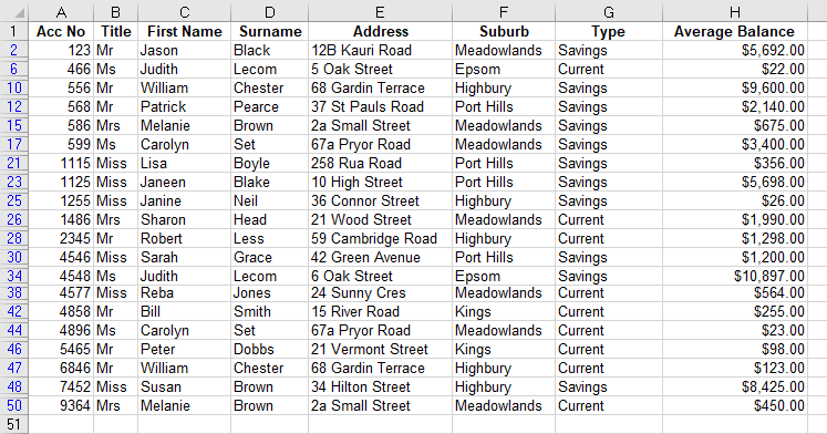
Consider the following worksheet.
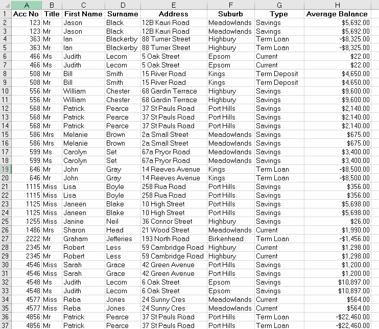
You can see at a glance that there are duplicates that you might wish to remove. The Type of account is a mixture of Saving, Term Loan and Check.
First you need to set up a criteria section for the advanced filter. You can do this in a separate sheet.
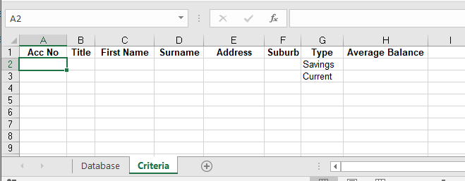
For ease of reference, I have named my data sheet ‘Database’ and my criteria sheet ‘Criteria’.
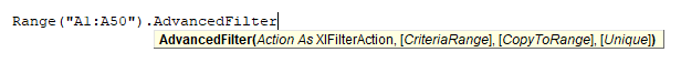
Advanced Filter Syntax
Expression.AdvancedFilter Action, CriteriaRange, CopyToRange, Unique
- The Expression represents the range object – and can be set as a Range (eg Range(“A1:A50”) – or the Range can be assigned to a variable and that variable can be used.
- The Action argument is required and will either be xlFilterInPlace or xlFilterCopy
- The Criteria Range argument is where you are getting the Criteria to filter from (our Criteria sheet above). This is optional as you would not need a criteria if you were filtering for unique values for example.
- The CopyToRange argument is where you are going to put your filter results – you can filter in place or you can have your filter result copied to an alternative location. This is also an optional argument.
- The Unique argument is also optional – True is to filter on unique records only, False is to filter on all the records that meet the criteria – if you omit this, the default will be False.
Filtering Data In Place
Using the criteria shown above in the criteria sheet – we want to find all the accounts with a type of ‘Savings’ and ‘Current’. We are filtering in place.
Sub CreateAdvancedFilter()
   Dim rngDatabase As Range
   Dim rngCriteria As Range
'define the database and criteria ranges
   Set rngDatabase = Sheets("Database").Range("A1:H50")
   Set rngCriteria = Sheets("Criteria").Range("A1:H3")
'filter the database using the criteria
   rngDatabase.AdvancedFilter xlFilterInPlace, rngCriteria
End Sub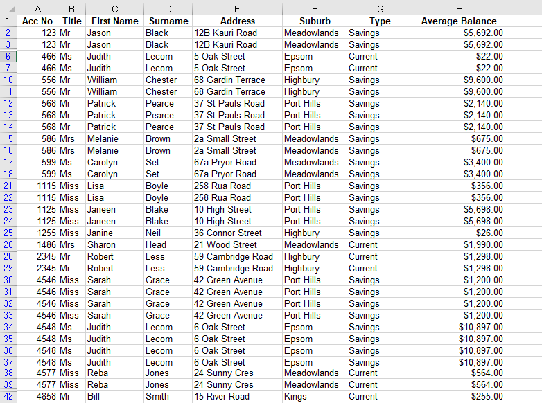
The code will hide the rows that do not meet the criteria.
In the above VBA procedure, we did not include the CopyToRange or Unique arguments.
Resetting the data
Before we run another filter, we have to clear the current one. This will only work if you have filtered your data in place.
Sub ClearFilter()
   On Error Resume Next
'reset the filter to show all the data
   ActiveSheet.ShowAllData
End Sub
Filtering Unique Values
In the procedure below, I have included the Unique argument but omitted the CopyToRange argument. If you leave this argument out, you EITHER have to put a comma as a place holder for the argument
Sub UniqueValuesFilter1()
   Dim rngDatabase As Range
   Dim rngCriteria As Range
'define the database and criteria ranges
   Set rngDatabase = Sheets("Database").Range("A1:H50")
   Set rngCriteria = Sheets("Criteria").Range("A1:H3")
'filter the database using the criteria
   rngDatabase.AdvancedFilter xlFilterInPlace, rngCriteria,,True
End Sub
OR you need to use named arguments as shown below.
Sub UniqueValuesFilter2()
Dim rngDatabase As Range
Dim rngCriteria As Range
'define the database and criteria ranges
Set rngDatabase = Sheets("Database").Range("A1:H50")
Set rngCriteria = Sheets("Criteria").Range("A1:H3")
'filter the database using the criteria
rngDatabase.AdvancedFilter Action:=xlFilterInPlace, CriteriaRange:=rngCriteria, Unique:=True
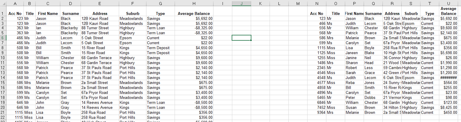
End SubBoth of the code examples above will run the same filter, as shown below – the data with only unique values.
Using the CopyTo argument
Sub CopyToFilter()
   Dim rngDatabase As Range
   Dim rngCriteria As Range
'define the database and criteria ranges
   Set rngDatabase = Sheets("Database").Range("A1:H50")
   Set rngCriteria = Sheets("Criteria").Range("A1:H3")
'copy the filtered data to an alternative location
    rngDatabase.AdvancedFilter Action:=xlFilterCopy, CriteriaRange:=rngCriteria, CopyToRange:=Range("N1:U1"), Unique:=True
End Sub
Note that we could have omitted the names of the arguments in the Advanced Filter line of code, but using named arguments does make the code easier to read and understand.
This line below is identical to the line in the procedure shown above.
rngDatabase.AdvancedFilter xlFilterCopy, rngCriteria, Range("N1:U1"), TrueOnce the code is run, the original data is still shown with the filtered data shown in the destination location specified in the procedure.
Removing Duplicates from the data
We can remove duplicates from the data by omitting the Criteria argument, and copying the data to a new location.
Sub RemoveDuplicates()
   Dim rngDatabase As Range
'define the database
   Set rngDatabase = Sheets("Database").Range("A1:H50")
'filter the database to a new range with unique set to true
rngDatabase.AdvancedFilter Action:=xlFilterCopy, CopyToRange:=Range("N1:U1"), Unique:=True
End Sub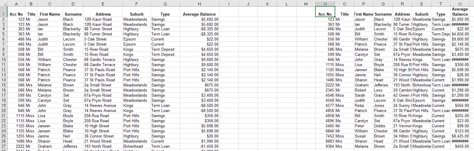
VBA Coding Made Easy
Stop searching for VBA code online. Learn more about AutoMacro — A VBA Code Builder that allows beginners to code procedures from scratch with minimal coding knowledge and with many time-saving features for all users!

Learn More!
Содержание
- Расширенный синтаксис фильтра
- Фильтрация данных на месте
- Сброс данных
- Фильтрация уникальных значений
- Использование аргумента CopyTo
- Удаление дубликатов из данных
В этом руководстве объясняется, как использовать метод расширенного фильтра в VBA.
Расширенная фильтрация в Excel очень полезна при работе с большими объемами данных, когда вы хотите применить несколько фильтров одновременно. Его также можно использовать для удаления дубликатов из ваших данных. Вы должны быть знакомы с созданием расширенного фильтра в Excel, прежде чем пытаться создать расширенный фильтр из VBA.
Рассмотрим следующий рабочий лист.

Вы можете сразу увидеть, что есть дубликаты, которые вы, возможно, захотите удалить. Тип счета представляет собой смесь сберегательного, срочного и чекового.
Сначала вам нужно настроить раздел критериев для расширенного фильтра. Сделать это можно на отдельном листе.

Для удобства я назвал свою таблицу данных «База данных», а таблицу критериев «Критерии».
Расширенный синтаксис фильтра
Expression.AdvancedFilter Action, CriteriaRange, CopyToRange, Unique

- В Выражение представляет объект диапазона — и может быть установлен как диапазон (например, Range («A1: A50»)) — или диапазон может быть назначен переменной, и эта переменная может использоваться.
- В Действие аргумент является обязательным и может иметь значение xlFilterInPlace или xlFilterCopy
- В Диапазон критериев аргумент — это то, откуда вы получаете критерии для фильтрации (наш лист критериев выше). Это необязательно, поскольку вам не понадобятся критерии, если вы, например, фильтруете уникальные значения.
- В CopyToRange Аргумент — это то место, куда вы собираетесь поместить результаты фильтра — вы можете фильтровать на месте или вы можете скопировать результат фильтра в альтернативное место. Это также необязательный аргумент.
- В Уникальный аргумент также является необязательным — Правда фильтровать только уникальные записи, Ложь — фильтровать все записи, соответствующие критериям — если вы его опустите, по умолчанию будет Ложь.
Фильтрация данных на месте
Используя критерии, указанные выше в таблице критериев, мы хотим найти все счета с типами «Сбережения» и «Текущие». Мы фильтруем на месте.
| 123456789 | Sub CreateAdvancedFilter ()Dim rngDatabase как диапазонDim rngCriteria As Range’определить базу данных и диапазоны критериевУстановите rngDatabase = Sheets («База данных»). Диапазон («A1: H50»)Установите rngCriteria = Sheets («Criteria»). Range («A1: H3»)’фильтровать базу данных по критериямrngDatabase.AdvancedFilter xlFilterInPlace, rngCriteriaКонец подписки |

Код скроет строки, не соответствующие критериям.
В приведенной выше процедуре VBA мы не включили аргументы CopyToRange или Unique.
Сброс данных
Перед тем, как запустить другой фильтр, мы должны очистить текущий. Это будет работать, только если вы отфильтровали свои данные на месте.
| 12345 | Sub ClearFilter ()При ошибке Возобновить Далее’сбросить фильтр, чтобы показать все данныеActiveSheet.ShowAllDataКонец подписки |
Фильтрация уникальных значений
В приведенной ниже процедуре я включил аргумент Unique, но опустил аргумент CopyToRange. Если вы опустите этот аргумент, вы ИЛИ нужно поставить запятую в качестве заполнителя для аргумента
| 123456789 | Sub UniqueValuesFilter1 ()Dim rngDatabase как диапазонDim rngCriteria As Range’определить базу данных и диапазоны критериевУстановите rngDatabase = Sheets («База данных»). Диапазон («A1: H50»)Установите rngCriteria = Sheets («Criteria»). Range («A1: H3»)’фильтруем базу данных по критериямrngDatabase.AdvancedFilter xlFilterInPlace, rngCriteria ,, ИстинаКонец подписки |
ИЛИ вам необходимо использовать именованные аргументы, как показано ниже.
| 123456789 | Sub UniqueValuesFilter2 ()Dim rngDatabase как диапазонDim rngCriteria As Range’определить базу данных и диапазоны критериевУстановите rngDatabase = Sheets («База данных»). Диапазон («A1: H50»)Установите rngCriteria = Sheets («Criteria»). Range («A1: H3»)’фильтруем базу данных по критериямrngDatabase.AdvancedFilter Действие: = xlFilterInPlace, CriteriaRange: = rngCriteria, Unique: = TrueКонец подписки |
Оба приведенных выше примера кода будут запускать один и тот же фильтр, как показано ниже — данные только с уникальными значениями.

Использование аргумента CopyTo
| 123456789 | Sub CopyToFilter ()Dim rngDatabase как диапазонDim rngCriteria As Range’определить базу данных и диапазоны критериевУстановите rngDatabase = Sheets («База данных»). Диапазон («A1: H50»)Установите rngCriteria = Sheets («Criteria»). Range («A1: H3»)’скопировать отфильтрованные данные в альтернативное местоrngDatabase.AdvancedFilter Action: = xlFilterCopy, CriteriaRange: = rngCriteria, CopyToRange: = Range («N1: U1»), Unique: = TrueКонец подписки |
Обратите внимание, что мы могли бы опустить имена аргументов в строке кода расширенного фильтра, но использование именованных аргументов делает код более легким для чтения и понимания.
Эта строка ниже идентична строке в процедуре, показанной выше.
| 1 | rngDatabase.AdvancedFilter xlFilterCopy, rngCriteria, Range («N1: U1»), True |
После запуска кода исходные данные по-прежнему отображаются с отфильтрованными данными, отображаемыми в месте назначения, указанном в процедуре.

Удаление дубликатов из данных
Мы можем удалить дубликаты из данных, опустив аргумент Criteria и скопировав данные в новое место.
| 1234567 | Sub RemoveDuplicates ()Dim rngDatabase как диапазон’определить базу данныхУстановите rngDatabase = Sheets («База данных»). Диапазон («A1: H50»)’фильтровать базу данных по новому диапазону с уникальным значением truerngDatabase.AdvancedFilter Action: = xlFilterCopy, CopyToRange: = Range («N1: U1»), Unique: = TrueКонец подписки |

Вы поможете развитию сайта, поделившись страницей с друзьями
A Powerful & Multi-purpose Templates for project management. Now seamlessly manage your projects, tasks, meetings, presentations, teams, customers, stakeholders and time. This page describes all the amazing new features and options that come with our premium templates.
Save Up to 85% LIMITED TIME OFFER

All-in-One Pack
120+ Project Management Templates
Essential Pack
50+ Project Management Templates
Excel Pack
50+ Excel PM Templates
PowerPoint Pack
50+ Excel PM Templates
MS Word Pack
25+ Word PM Templates
Ultimate Project Management Template
Ultimate Resource Management Template
Project Portfolio Management Templates
- Excel VBA Range Advanced Filter – Syntax
- Excel VBA Range Advanced Filter- Examples
- Excel VBA Range Advanced Filter- Instructions
- Real-time Applications on Excel VBA Range Advanced Filters
-
- Excel Template for Monthly Expenses
- Excel Template for Task Management
- How to Use Project Plan Template
- VBA ActiveSheet – Excel Active Sheet Object
- Excel VBA ColorIndex
- Excel VBA Copy Range to Another Sheet with Formatting
- VBA Filter Multiple Columns
- VBA Filter Column
- VBA Autofilter – Excel Explained with Examples
- Invoice Template Excel – Free Download
-
Page load link
Go to Top
Когда вы работаете с большими объемами данных, нельзя представить себе эту деятельность без фильтров. Однозначно, что в Excel разработан очень мощный и удобный инструмент фильтрации, который позволяет выбирать определенные данные из диапазона. А с приходом Excel 2007 добавилась возможность выбирать данные с определенной заливкой. Все это облегчает рабочие будни Excel юзеров и упрощает жизнь. Однако, есть еще один элемент, который пока еще не реализован в стандартных фильтрах Excel, но приятно было бы иметь в арсенале, я говорю о фильтрации с помощью символов подстановки, который мы попытаемся сегодня реализовать с помощью VBA.
Оригинальную статью можно найти на сайте https://yoursumbuddy.com/
В данной статье описан способ создания фильтра на основе формы ListBox на VBA. Фильтр использует оператор Like, для поиска соответствий в заданном диапазоне. К примеру, набрав в фильтре celti, программа вернет мне значение Exceltip, но это не самое главное, так как стандартный фильтр позволяет проводить подобные манипуляции. Гораздо интереснее, что оператор Like позволяет использовать символы подстановки, таким образом введя в текстовое поле значение /*/201? , Excel вернет все даты начиная с 2010 года. Плюс ко всему, данный фильтр позволяет задавать чувствительность к регистру и отбирать уникальные значения.
Внизу показаны принципы работы фильтра на примере списка женских имен с добавлением выбора уникальных значений и чувствительности к регистру. Обратите внимание, щелчок на имени в фильтре позволяет выбирать его в списке.
Ниже отображен макрос, который запускается каждый раз, когда меняется значение в текстовом поле фильтра или происходит щелчок на один из элементов списка в фильтре.
|
1 |
Sub ResetFilter() ‘звездочка возвращает все значения списка UniqueValuesOnly = Me.chkUnique.Value ‘используется, если Уникальные значения равно ИСТИНА If Not UniqueConstraint Then |
В этом макросе использована возможность элемента Collection хранить только уникальные значения. Если на форме установлена галочка Уникальные, то макрос проверит его прежде, чем поместит в массив ListBox.
Переменная FilterPattern имеет звездочки в начале и конце строки. Это позволяет находить записи внутри таблицы.
В дополнение, массив с женскими именами хранит порядковый номер этого имени, что позволяет запускать другой макрос, который выделяет соответствующую ячейку в таблице при выделении имени в форме.
|
1 |
Private Sub lstDetail_Change() Sub GoToRow() |
Скорость макроса достаточно приемлема для таблиц с менее чем 10000 строками. Но даже с превышением этого порога, макрос будет работать, главное, чтобы число строк было менее 65536.
Для лучшего понимания прикладываю файл с макросом.