
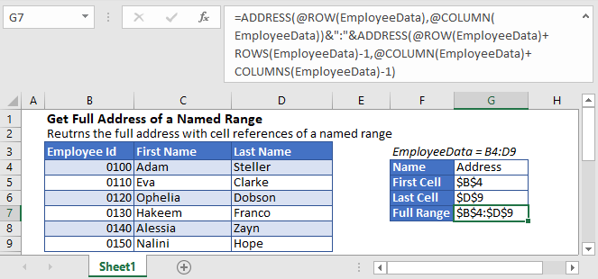
This tutorial will demonstrate how to get the full address of a named range in Excel & Google Sheets.
Named Ranges
A Named Range is a range of a single cell or multiple cells, which are assigned a specific name. Named Ranges are one of Microsoft Excel’s useful features; they can make formulae easier to understand.
Get Address of Named Range
To get the full address of a named range, you can use an Excel formula that contains ADDRESS, ROW, ROWS, COLUMN, and COLUMNS functions.
In order to get the full address of a named range, we’ll find the first and last cell references of the named range and then join them together with a colon (“:”).
Get First Cell Address in a Named Range
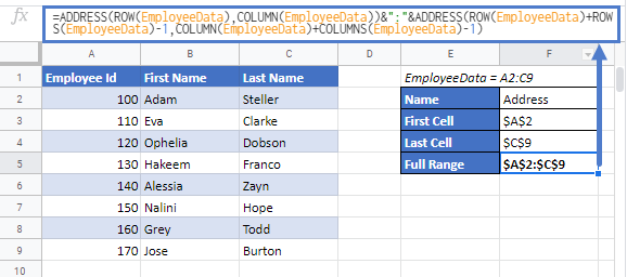
Let’s say we have a named range “EmployeeData” in range B4:D9.
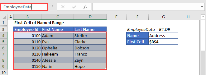
To get the cell reference of the first cell in a named range, we’ll use the ADDRESS function together with ROW and COLUMN functions:
=ADDRESS(ROW(EmployeeData),COLUMN(EmployeeData))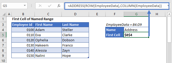
The ADDRESS function returns the address of a specific row and column. We use the ROW and COLUMN Functions to calculate the first row and column in the named range, plugging the results into the ADDRESS Function. The Result is the first cell in the named range.
The above formula has returned the absolute cell reference ($B$4). But if you want a relative address(without $ sign, B4), you need to supply 4 for the third (optional) argument of the ADDRESS function like this:
=ADDRESS(ROW(EmployeeData),COLUMN(EmployeeData),4)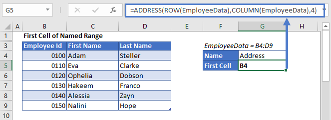
Get Last Cell Address in a Named Range
To get the cell reference of the last cell in a named range, we can use the following formula:
=ADDRESS(ROW(EmployeeData)+ROWS(EmployeeData)-1,COLUMN(EmployeeData)+COLUMNS(EmployeeData)-1)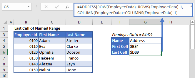
Here the ROWS and COLUMNS Functions count the number of rows and columns in the range, which we add to the original formula above, returning the last cell in the named range.
Similarly, if you want a relative address instead of an absolute cell reference, you can supply 4 for the third argument in the ADDRESS function like this:
=ADDRESS(ROW(EmployeeData)+ROWS(EmployeeData)-1,COLUMN(EmployeeData)+COLUMNS(EmployeeData)-1,4)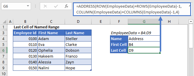
Full Address of Named Range
Now in order to get the complete address of a named range, we’ll just have to concatenate the above two formulas with the operator (:), in the above example like this:
=ADDRESS(ROW(EmployeeData),COLUMN(EmployeeData))&":"&ADDRESS(ROW(EmployeeData)+ROWS(EmployeeData)-1,COLUMN(EmployeeData)+COLUMNS(EmployeeData)-1)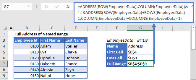
Similarly, to return the address of the named range as a relative reference (without $ sign), supply the third argument of the ADDRESS functions with 4, like this:
=ADDRESS(ROW(EmployeeData),COLUMN(EmployeeData),4)&":"&ADDRESS(ROW(EmployeeData)+ROWS(EmployeeData)-1,COLUMN(EmployeeData)+COLUMNS(EmployeeData)-1,4)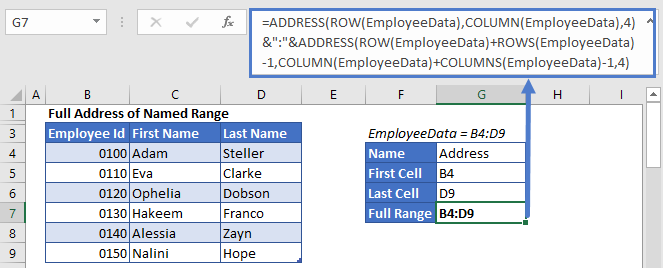
Get Full Address of a Named Range in Google Sheets
The formula to get the full address of a named range works exactly the same in Google Sheets as in Excel:
How to use VBA Range.Address method?
Range.Address is used to get the cell address for simple local reference (ex. $A$1) or reference style notation for cell references (ex. A1 or R1C1 format). It can also be used to get the range address which includes the workbook name and worksheet name.
Syntax
expression .Address(RowAbsolute, ColumnAbsolute, ReferenceStyle, External, RelativeTo)
expression A variable that represents a Range object.
Parameters
| Name | Required/Optional | Data Type | Description | ||
| RowAbsolute | Optional | Variant |
|
||
| ColumnAbsolute | Optional | Variant | True to return the column part of the reference as an absolute reference. The default value is True. | ||
| ReferenceStyle | Optional | XlReferenceStyle | The reference style. The default value is xlA1. | ||
| External | Optional | Variant |
|
||
| RelativeTo | Optional | Variant | If RowAbsolute and ColumnAbsolute are False, and ReferenceStyle is xlR1C1, you must include a starting point for the relative reference. This argument is a Range object that defines the starting point. |
Below are the different sample codes:
- To simply display the local reference of the cell address
Sub Range_Address1() Set MyRange = Worksheets("021817").Cells(1, 1) MsgBox MyRange.Address() ' $A$1 End Sub
- To simply display the absolute address of the cell
Sub Range_Address2() Set MyRange = Worksheets("021817").Cells(1, 1) MsgBox MyRange.Address(RowAbsolute:=False) ' $A1 End Sub
- To display the reference style of the cell address. This simply means using the combination of both column letter and row number.
Sub Range_Address3() Set MyRange = Worksheets("021817").Cells(1, 1) MsgBox MyRange.Address(ReferenceStyle:=xlR1C1) ' R1C1 End Sub
- To display the cell address including workbook and worksheet name
Sub Range_Address4() Set MyRange = Worksheets("021817").Cells(1, 1) MsgBox MyRange.Address(External:=True) 'Address includes workbook and worksheet name End Sub
- Using the combined parameters
Sub Range_Address5() Set MyRange = Worksheets("021817").Cells(1, 1) MsgBox MyRange.Address(ReferenceStyle:=xlR1C1, _ RowAbsolute:=False, _ ColumnAbsolute:=False, _ RelativeTo:=Worksheets(1).Cells(3, 3)) ' R[-2]C[-2] End Sub
The Excel ADDRESS function returns a cell reference as a string, based on a row and column number
Example: Excel ADDRESS Function

METHOD 1. Excel ADDRESS function using hardcoded values
EXCEL
|
Result in cell G5 ($D$3) — returns the assigned cell reference that comprises only the required ADDRESS arguments (row number and column number)) as a string. |
|
Result in cell G6 ($D$3) — returns the assigned cell reference that comprises the required ADDRESS arguments (row number and column number) and an abs number (Absolute row and column) as a string. |
|
Result in cell G7 (D$3) — returns the assigned cell reference that comprises the required ADDRESS arguments (row number and column number) and an abs number (Absolute row and Relative column) as a string. |
|
Result in cell G8 ($D3) — returns the assigned cell reference that comprises the required ADDRESS arguments (row number and column number) and an abs number (Relative row and Absolute column) as a string. |
|
Result in cell G9 (D3) — returns the assigned cell reference that comprises the required ADDRESS arguments (row number and column number) and an abs number (Relative row and column) as a string. |
|
Result in cell G10 ($D$3) — returns the assigned cell reference that comprises the required ADDRESS arguments (row number and column number), abs number (Absolute row and column) and A1 reference style as a string. |
|
Result in cell G11 ($D$3) — returns the assigned cell reference that comprises the required ADDRESS arguments (row number and column number) and A1 reference style as a string. |
|
Result in cell G12 (R3C3) — returns the assigned cell reference that comprises the required ADDRESS arguments (row number and column number), abs number (Absolute row and column) and R1C1 reference style as a string. |
|
=ADDRESS(3,4,1,TRUE,»Sheet1″) |
Result in cell G13 (Sheet1!$D$3) — returns the assigned cell reference that comprises the required ADDRESS arguments (row number and column number), abs number (Absolute row and column), A1 reference style and reference a sheet name as a string. |
METHOD 2. Excel ADDRESS function using links
EXCEL
|
Result in cell G5 ($D$3) — returns the assigned cell reference that comprises only the required ADDRESS arguments (row number and column number)) as a string. |
|
Result in cell G6 ($D$3) — returns the assigned cell reference that comprises the required ADDRESS arguments (row number and column number) and an abs number (Absolute row and column) as a string. |
|
Result in cell G7 (D$3) — returns the assigned cell reference that comprises the required ADDRESS arguments (row number and column number) and an abs number (Absolute row and Relative column) as a string. |
|
Result in cell G8 ($D3) — returns the assigned cell reference that comprises the required ADDRESS arguments (row number and column number) and an abs number (Relative row and Absolute column) as a string. |
|
Result in cell G9 (D3) — returns the assigned cell reference that comprises the required ADDRESS arguments (row number and column number) and an abs number (Relative row and column) as a string. |
|
Result in cell G10 ($D$3) — returns the assigned cell reference that comprises the required ADDRESS arguments (row number and column number), abs number (Absolute row and column) and A1 reference style as a string. |
|
Result in cell G11 ($D$3) — returns the assigned cell reference that comprises the required ADDRESS arguments (row number and column number) and A1 reference style as a string. |
|
Result in cell G12 (R3C3) — returns the assigned cell reference that comprises the required ADDRESS arguments (row number and column number), abs number (Absolute row and column) and R1C1 reference style as a string. |
|
=ADDRESS(B13,C13,D13,E13,F13) |
Result in cell G13 (Sheet1!$D$3) — returns the assigned cell reference that comprises the required ADDRESS arguments (row number and column number), abs number (Absolute row and column), A1 reference style and reference a sheet name as a string. |
METHOD 3. Excel ADDRESS function using the Excel built-in function library with hardcoded value
EXCEL
Formulas tab > Function Library group > Lookup & Reference > ADDRESS > populate the input boxes
| = ADDRESS(3,4,1,TRUE,»Sheet1″) Note: in this example we are populating all of the input boxes associated with the ADDRESS function arguments, however, you are only required to populate the required arguments (Row_num and Column_num). You can omit the optional arguments and Excel will apply its default value against each of them. |
 |
METHOD 4. Excel ADDRESS function using the Excel built-in function library with links
EXCEL
Formulas tab > Function Library group > Lookup & Reference > ADDRESS > populate the input boxes
| = ADDRESS(B13,C13,D13,E13,F13) Note: in this example we are populating all of the input boxes associated with the ADDRESS Function arguments with links, however, you are only required to populate the required arguments (Row_num and Column_num). You can omit the optional arguments and Excel will apply the default value against each of them. |
 |
METHOD 1. Excel ADDRESS function using VBA with hardcoded values
VBA
Sub Excel_ADDRESS_Function_Using_Hardcoded_Values()
‘declare a variable
Dim ws As Worksheet
Set ws = Worksheets(«ADDRESS»)
‘apply the Excel ADDRESS function
ws.Range(«G5») = ws.Cells(3, 4).Address()
ws.Range(«G6») = ws.Cells(3, 4).Address(RowAbsolute:=True)
ws.Range(«G7») = ws.Cells(3, 4).Address(ColumnAbsolute:=False)
ws.Range(«G8») = ws.Cells(3, 4).Address(RowAbsolute:=False)
ws.Range(«G9») = ws.Cells(3, 4).Address(RowAbsolute:=False, ColumnAbsolute:=False)
ws.Range(«G10») = ws.Cells(3, 4).Address(RowAbsolute:=True, ReferenceStyle:=xlA1)
ws.Range(«G11») = ws.Cells(3, 4).Address(ReferenceStyle:=xlA1)
ws.Range(«G12») = ws.Cells(3, 4).Address(RowAbsolute:=True, ReferenceStyle:=xlR1C1)
ws.Range(«G13») = «‘» & ThisWorkbook.Worksheets(«Sheet1»).Cells(1, 1).Parent.Name & «‘!» & ws.Cells(3, 4).Address(RowAbsolute:=True)
End Sub
OBJECTS
Range: The Range object is a representation of a single cell or a range of cells in a worksheet.
Worksheets: The Worksheets object represents all of the worksheets in a workbook, excluding chart sheets.
PREREQUISITES
Worksheet Name: Have a worksheet named ADDRESS.
ADJUSTABLE PARAMETERS
Output Range: Select the output range by changing the cell references («G5»), («G6»), («G7»), («G8»), («G9»), («G10»), («G11»), («G12») and («G13») in the VBA code to any cell in the worksheet, that doesn’t conflict with the formula.
METHOD 2. Excel ADDRESS function using VBA with links
VBA
Sub Excel_ADDRESS_Function_Using_Links()
‘declare a variable
Dim ws As Worksheet
Set ws = Worksheets(«ADDRESS»)
‘apply the Excel ADDRESS function
ws.Range(«G5») = ws.Cells(Range(«B5»), Range(«C5»)).Address()
ws.Range(«G6») = ws.Cells(Range(«B6»), Range(«C6»)).Address(RowAbsolute:=True)
ws.Range(«G7») = ws.Cells(Range(«B7»), Range(«C7»)).Address(ColumnAbsolute:=False)
ws.Range(«G8») = ws.Cells(Range(«B8»), Range(«C8»)).Address(RowAbsolute:=False)
ws.Range(«G9») = ws.Cells(Range(«B9»), Range(«C9»)).Address(RowAbsolute:=False, ColumnAbsolute:=False)
ws.Range(«G10») = ws.Cells(Range(«B10»), Range(«C10»)).Address(RowAbsolute:=True, ReferenceStyle:=xlA1)
ws.Range(«G11») = ws.Cells(Range(«B11»), Range(«C11»)).Address(ReferenceStyle:=xlA1)
ws.Range(«G12») = ws.Cells(Range(«B12»), Range(«C12»)).Address(RowAbsolute:=True, ReferenceStyle:=xlR1C1)
ws.Range(«G13») = «‘» & ThisWorkbook.Worksheets(«Sheet1»).Cells(1, 1).Parent.Name & «‘!» & ws.Cells(Range(«B13»), Range(«C13»)).Address(RowAbsolute:=True)
End Sub
OBJECTS
Range: The Range object is a representation of a single cell or a range of cells in a worksheet.
Worksheets: The Worksheets object represents all of the worksheets in a workbook, excluding chart sheets.
PREREQUISITES
Worksheet Name: Have a worksheet named ADDRESS.
ADJUSTABLE PARAMETERS
Output Range: Select the output range by changing the cell references («G5»), («G6»), («G7»), («G8»), («G9»), («G10»), («G11»), («G12») and («G13») in the VBA code to any cell in the worksheet, that doesn’t conflict with the formula.
METHOD 3. Excel ADDRESS function using VBA with ranges
VBA
Sub Excel_ADDRESS_Function_Using_Ranges()
‘declare a variable
Dim ws As Worksheet
Set ws = Worksheets(«ADDRESS»)
‘apply the Excel ADDRESS function
ws.Range(«G5») = ws.Range(«D3»).Address()
ws.Range(«G6») = ws.Range(«D3»).Address(RowAbsolute:=True)
ws.Range(«G7») = ws.Range(«D3»).Address(ColumnAbsolute:=False)
ws.Range(«G8») = ws.Range(«D3»).Address(RowAbsolute:=False)
ws.Range(«G9») = ws.Range(«D3»).Address(RowAbsolute:=False, ColumnAbsolute:=False)
ws.Range(«G10») = ws.Range(«D3»).Address(RowAbsolute:=True, ReferenceStyle:=xlA1)
ws.Range(«G11») = ws.Range(«D3»).Address(ReferenceStyle:=xlA1)
ws.Range(«G12») = ws.Range(«D3»).Address(RowAbsolute:=True, ReferenceStyle:=xlR1C1)
ws.Range(«G13») = «‘» & ThisWorkbook.Worksheets(«Sheet1»).Cells(1, 1).Parent.Name & «‘!» & ws.Range(«D3»).Address(RowAbsolute:=True)
End Sub
OBJECTS
Range: The Range object is a representation of a single cell or a range of cells in a worksheet.
Worksheets: The Worksheets object represents all of the worksheets in a workbook, excluding chart sheets.
PREREQUISITES
Worksheet Name: Have a worksheet named ADDRESS.
ADJUSTABLE PARAMETERS
Output Range: Select the output range by changing the cell references («G5»), («G6»), («G7»), («G8»), («G9»), («G10»), («G11»), («G12») and («G13») in the VBA code to any cell in the worksheet, that doesn’t conflict with the formula.
Usage of the Excel ADDRESS function and formula syntax
EXPLANATION
DESCRIPTION
The Excel ADDRESS function returns a cell reference as a string, based on a row and column number.
SYNTAX
=ADDRESS(row_num, column_num, [abs_num],[a1],[sheet_text])
ARGUMENT(S)
row_num: (Required) Row number to use in the reference.
column_num: (Required) Column number to use in the reference.
abs_num: (Optional) Type of address reference to use. This can be any of the following values:
| Value | Explanation | Example |
|---|---|---|
| 1 | Absolute row and column | $A$1 |
| 2 | Absolute row and Relative column | A$1 |
| 3 | Relative row and Absolute column | $A1 |
| 4 | Relative row and column | A1 |
Note: If the abs_num argument is omitted, the default value is 1 (Absolute row and column).
a1: (Optional) Specifies what type of reference style to use. This can be any of the following:
| Value | Explanation | Example |
|---|---|---|
| TRUE | A1 reference style | A1, A2, B2 |
| FALSE | R1C1 reference style | R1C1, R2C1, R2C2 |
Note: If the a1 argument is omitted, the default value is TRUE (A1 reference style).
sheet_text: (Optional) Specifies the name of the worksheet to be used. You will need to insert the name between the quotation marks («Name»).
Note: If the sheet_text argument is omitted, no sheet name will appear.
In this example the goal is to return the full address of a range or named range as text. The purpose of this formula is informational, not functional. It provides a way to inspect the current range for a named range, an Excel Table, or even the result of a formula. The core of the solutions explained below is the ADDRESS function, which returns a cell address based on a given row and column. The formula gets somewhat complicated because we need to use ADDRESS twice, and because there is a lot of busy work in collecting the coordinates we need to provide to ADDRESS. See below for a more elegant formula that takes advantage of the LET function and the TAKE function in Excel 365. This version can also report the range returned by another function (like OFFSET).
Note: the CELL function is another way to get the address for a cell. However, CELL does not provide a way to choose a relative or absolute format like the ADDRESS function does. In addition, CELL is a volatile function and can cause performance problems in large or complex worksheets. For those reasons, I have avoided it in this example.
Background
The links below provide more details about Excel Tables and named ranges:
- How to create an Excel Table (video)
- How to create a named range (video)
- How to create a dynamic named range with a table (video)
Demo
The animation below shows how the formula responds when a Table named «data» is resized. In the worksheet, DA stands for Dynamic Array version of Excel and Legacy stands for older versions of Excel. See below for more information about the dynamic array version.

The basic idea
The basic idea of this formula is to get the coordinates of the first (upper left) cell in a range and the last (lower right) cell in a range, then use these coordinates to create cell references, then join the references together with concatenation. The formula itself looks complicated and scary:
=ADDRESS(@ROW(data),@COLUMN(data),4)&":"&ADDRESS(@ROW(data)+ROWS(data)-1,@COLUMN(data)+COLUMNS(data)-1,4)However, most of what you see is the «busy work» of collecting the coordinates with the ROW, ROWS, COLUMN, and COLUMNS functions. Once that work is done, the formula simplifies to this:
=ADDRESS(5,2,4)&":"&ADDRESS(16,4,4)The ADDRESS function then creates a reference to the first and last cell in the range, and the two references are joined together. That’s it. The rest of the problem is the details of collecting the coordinates needed by the ADDRESS function.
ROW and COLUMN functions
The ROW and COLUMN functions simply return coordinates. For example, if we give ROW and COLUMN cell B5 as a reference, we get back coordinate numbers:
=ROW(B5) // returns 5
=COLUMN(B5) // returns 2
Notice that COLUMN returns a number, not a letter: column A, is 1, column B is 2, column C is 3, etc.
ROWS and COLUMNS functions
The ROWS and COLUMNS functions return counts. For example, if we give ROWS and COLUMNS the range B5:D16, we get back the number of rows and the number of columns in the range:
=ROWS(B5:D16) // returns 12
=COLUMNS(B5:D16) // returns 3
ADDRESS function
The ADDRESS function returns the address for a cell based on a given row and column number as text. For example:
=ADDRESS(1,1) // returns "$A$1"
=ADDRESS(5,2) // returns "$B$5"
Note that ADDRESS returns an address as an absolute reference by default. However, by providing 4 for the optional argument abs_num, ADDRESS will return a relative reference:
=ADDRESS(1,1,4) // returns "A1"
=ADDRESS(5,2,4) // returns "B5"
In this problem, we need to build up an address for a range in two parts (1) a reference to the first cell in the range and (2) a reference to the last cell in a range. To get the address for the first cell in the range, we use this formula:
=ADDRESS(@ROW(data),@COLUMN(data))
Note: data is the named range B5:E16.
As mentioned above, the ROW function and the COLUMN function return coordinates: ROW returns a row number, and COLUMN returns a column number. In this case however, we are giving ROW and COLUMN the range data, not a single cell. As a result, we get back an array of numbers:
=ROW(data) // returns {5;6;7;8;9;10;11;12;13;14;15;16}
=COLUMN(data) // returns {2,3,4,5}
In other words, ROW returns all row numbers for data (B5:D15), and COLUMN returns all column numbers for data. This is where the formula gets a bit complicated due to Excel version differences.
Although ROW and COLUMN return multiple results, older versions of Excel will automatically limit the results to the first value only. This works fine for the problem at hand, because we only want the first value. However, in the dynamic version of Excel, multiple results are not automatically limited, because formulas can spill results onto the worksheet. We don’t want this behavior in this case, so we use the implicit intersection operator (@) to limit the output from ROW and COLUMN to one value only:
=@ROW(data) // returns 5
=@COLUMN(data) // returns 2
In effect, this mimics the behavior in Legacy Excel where formulas that return more than one result display one result only. Note that the implicit intersection operator (@) is not required in Legacy Excel. In fact, if you try to add the @ in an older version of Excel, Excel will simply remove it. However, it is required in the current version of Excel.
Returning to the formula, ROW and COLUMN return their results directly to ADDRESS as the row_num and column_num arguments. With abs_num provided as 4 (relative), ADDRESS returns the text «B5».
=ADDRESS(5,2,4) // returns "B5"
To get the last cell in the range, we use the ADDRESS function again like this:
ADDRESS(@ROW(data)+ROWS(data)-1,@COLUMN(data)+COLUMNS(data)-1,4)
Essentially, we follow the same idea as above, using ROW and COLUMN to get the last row and last column of the range. However we also calculate the total number of rows with the ROWS function and the total number of columns with the COLUMNS function:
=ROWS(data) // returns 12
=COLUMNS(data) // returns 4
Then we do some simple math to calculate the row and column number of the last cell. We add the row count to the starting row, and add the column count to the starting column, then subtract 1 to get the correct coordinates for the last cell:
=ADDRESS(@ROW(data)+ROWS(data)-1,@COLUMN(data)+COLUMNS(data)-1,4)
=ADDRESS(5+12-1,2+4-1,4)
=ADDRESS(16,5,4)
="E16"
With abs_num set to 4. ADDRESS returns «E16», the address of the last cell in data as text. At this point, we have the address for the first cell and the address for the last cell. The only thing left to do is concatenate them together separated by a colon:
="B5"&":"&"E16"
="B5:E16"
More elegant formula
Although the formula above works fine, it is cumbersome and redundant. New array functions in Excel make it possible to solve the problem with a more elegant formula like this:
=LET(
first,TAKE(rng,1,1),
last,TAKE(rng,-1,-1),
ADDRESS(ROW(first),COLUMN(first),4)&":"&
ADDRESS(ROW(last),COLUMN(last),4)
)
Where rng is the generic placeholder for a named range or Excel Table. In this formula, the LET function is used to assign values to two variables: first and last. First represents the first cell in the range and last represents the last cell in the range. These values are assigned with the TAKE function like this:
first,TAKE(rng,1,1), // first cell (B5)
last,TAKE(rng,-1,-1), // last cell (E16)
The TAKE function returns a subset of a given array or range. The size of the array returned is determined by separate rows and columns arguments. When positive numbers are provided for rows or columns, TAKE returns values from the start or top of the array. Negative numbers take values from the end or bottom of the array. What’s tricky about this, and not obvious, is that when working with ranges, TAKE returns a valid reference. You don’t normally see the reference because as with most formulas, Excel returns the value at that reference, not the reference itself. However, the reference is there, as is obvious in the next step.
Finally, the ADDRESS function is used to generate an address for both the first cell and the last cell in the range, and the two results are concatenated with a colon (:) in between:
ADDRESS(ROW(first),COLUMN(first),4)&":"&ADDRESS(ROW(last),COLUMN(last),4)
Substituting the references returned by TAKE, the formula evaluates like this:
=ADDRESS(ROW(B5),COLUMN(B5),4)&":"&ADDRESS(ROW(E16),COLUMN(E16),4)
=ADDRESS(5,2,4)&":"&ADDRESS(16,4,4)
="B5"&":"&"E16"
="B5:E16"
Named range as text
To get an address for a named range entered as a text value (i.e. «range», «data», etc.), you’ll need to use the INDIRECT function to change the text into a valid reference before proceeding. For example, to get the address of a table name entered in A1 as text, you could use this unwieldy formula:
=ADDRESS(ROW(INDIRECT(A1)),COLUMN(INDIRECT(A1)))&":"&ADDRESS(ROW(INDIRECT(A1))+ROWS(INDIRECT(A1))-1,COLUMN(INDIRECT(A1))+COLUMNS(INDIRECT(A1))-1)
In the dynamic array version of Excel, the LET function makes this much simpler. With a range or table name as text in cell A1, you can call INDIRECT just once like this:
=LET(
rng,INDIRECT(A1),
first,TAKE(rng,1,1),
last,TAKE(rng,-1,-1),
ADDRESS(ROW(first),COLUMN(first),4)&":"&
ADDRESS(ROW(last),COLUMN(last),4)
)
You can read more about the LET function here.
Named LAMBDA option
Taking things a step further, you can use the LAMBDA function to create a custom function like this:
=LAMBDA(range,
  LET(
    rng,IF(ISREF(range),range,INDIRECT(range)),
    first,TAKE(rng,1,1),
    last,TAKE(rng,-1,-1),
    ADDRESS(ROW(first),COLUMN(first),4)&":"&
    ADDRESS(ROW(last),COLUMN(last),4)
  )
)(data)
This version of the formula does the same thing as the formula above with one additional step: it checks for range or table names entered as text values. This is done with the ISREF function in the first step. If the value passed in for range is a valid reference, we use it as-is to assign a value to rng. If not, we run it through the INDIRECT function to try and get a valid reference.
Finally, if we give the LAMBDA formula above the name «GetRange», we can call it on any valid range like this:
=GetRange(data)Read more about creating and naming custom LAMBDA formulas here.
Check reference returned by formula
A nice feature of the LAMBDA version of the formula is we easily can use it to check the result of any formula that returns a range. For example, we can call it with the OFFSET function like this:
=GetRange(OFFSET(A1,4,1,10,2)) // returns "B5:C14"The point here is that it is not easy to understand what range is returned by OFFSET, because Excel will return only the values in the range. The custom GetRange function makes it possible to print the range returned by a formula explicitly.
Other ideas
I looked at two other formulas to solve this problem. The first uses ADDRESS and TAKE:
=LET(
d,ADDRESS(ROW(data),COLUMN(data),4),
TAKE(a,1,1)&":"&TAKE(a,-1,-1)
)
The second uses ADDRESS and the new TOCOL function:
=LET(
d,TOCOL(ADDRESS(ROW(data),COLUMN(data),4)),
INDEX(d,1)&":"&INDEX(d,ROWS(d))
)
Both formulas use the ADDRESS function to spin up all of the addresses in the range at the same time. The first formula then uses the TAKE function to get the first and last address. The second formula uses the TOCOL function to unwrap the array of references created by ADDRESS, then it uses the INDEX function twice to get the first and the last value. On small ranges, these formulas should work nicely. However, on very large ranges you are likely to see a performance hit because of time needed to create all of the extra addresses. The proposes formula solution above avoids this problem by only creating the first and last reference. The tradeoff is that the formula is more complex.
The VBA Range Object
The Excel Range Object is an object in Excel VBA that represents a cell, row, column, a selection of cells or a 3 dimensional range. The Excel Range is also a Worksheet property that returns a subset of its cells.
Worksheet Range
The Range is a Worksheet property which allows you to select any subset of cells, rows, columns etc.
Dim r as Range 'Declared Range variable

Set r = Range("A1") 'Range of A1 cell

Set r = Range("A1:B2") 'Square Range of 4 cells - A1,A2,B1,B2

Set r= Range(Range("A1"), Range ("B1")) 'Range of 2 cells A1 and B1

Range("A1:B2").Select 'Select the Cells A1:B2 in your Excel Worksheet

Range("A1:B2").Activate 'Activate the cells and show them on your screen (will switch to Worksheet and/or scroll to this range.
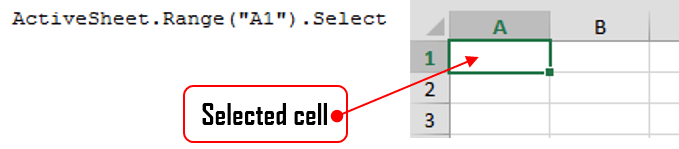
Select a cell or Range of cells using the Select method. It will be visibly marked in Excel:
Working with Range variables
The Range is a separate object variable and can be declared as other variables. As the VBA Range is an object you need to use the Set statement:
Dim myRange as Range
'...
Set myRange = Range("A1") 'Need to use Set to define myRange
The Range object defaults to your ActiveWorksheet. So beware as depending on your ActiveWorksheet the Range object will return values local to your worksheet:
Range("A1").Select
'...is the same as...
ActiveSheet.Range("A1").Select
You might want to define the Worksheet reference by Range if you want your reference values from a specifc Worksheet:
Sheets("Sheet1").Range("A1").Select 'Will always select items from Worksheet named Sheet1
The ActiveWorkbook is not same to ThisWorkbook. Same goes for the ActiveSheet. This may reference a Worksheet from within a Workbook external to the Workbook in which the macro is executed as Active references simply the currently top-most worksheet. Read more here
Range properties
The Range object contains a variety of properties with the main one being it’s Value and an the second one being its Formula.
A Range Value is the evaluated property of a cell or a range of cells. For example a cell with the formula =10+20 has an evaluated value of 20.
A Range Formula is the formula provided in the cell or range of cells. For example a cell with a formula of =10+20 will have the same Formula property.
'Let us assume A1 contains the formula "=10+20"

Debug.Print Range("A1").Value 'Returns: 30

Debug.Print Range("A1").Formula 'Returns: =10+20
Other Range properties include:
Work in progress
Worksheet Cells
A Worksheet Cells property is similar to the Range property but allows you to obtain only a SINGLE CELL, based on its row and column index. Numbering starts at 1:

The Cells property is in fact a Range object not a separate data type.
Excel facilitates a Cells function that allows you to obtain a cell from within the ActiveSheet, current top-most worksheet.
Cells(2,2).Select 'Selects B2
'...is the same as...
ActiveSheet.Cells(2,2).Select 'Select B2
Cells are Ranges which means they are not a separate data type:
Dim myRange as Range
Set myRange = Cells(1,1) 'Cell A1
Range Rows and Columns
As we all know an Excel Worksheet is divided into Rows and Columns. The Excel VBA Range object allows you to select single or multiple rows as well as single or multiple columns. There are a couple of ways to obtain Worksheet rows in VBA:
Getting an entire row or column
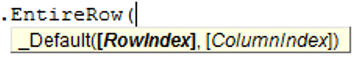
 To get and entire row of a specified Range you need to use the EntireRow property. Although, the function’s parameters suggest taking both a RowIndex and ColumnIndex it is enough just to provide the row number. Row indexing starts at 1.
 To get and entire column of a specified Range you need to use the EntireColumn property. Although, the function’s parameters suggest taking both a RowIndex and ColumnIndex it is enough just to provide the column number. Column indexing starts at 1.
Range("B2").EntireRows(1).Hidden = True 'Gets and hides the entire row 2

Range("B2").EntireColumns(1).Hidden = True 'Gets and hides the entire column 2
The three properties EntireRow/EntireColumn, Rows/Columns and Row/Column are often misunderstood so read through to understand the differences.
Get a row/column of a specified range
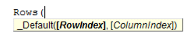 If you want to get a certain row within a Range simply use the Rows property of the Worksheet. Although, the function’s parameters suggest taking both a RowIndex and ColumnIndex it is enough just to provide the row number. Row indexing starts at 1.
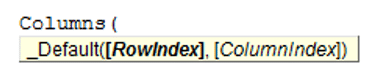 Similarly you can use the Columns function to obtain any single column within a Range. Although, the function’s parameters suggest taking both a RowIndex and ColumnIndex actually the first argument you provide will be the column index. Column indexing starts at 1.
Rows(1).Hidden = True 'Hides the first row in the ActiveSheet
'same as
ActiveSheet.Rows(1).Hidden = True

Columns(1).Hidden = True 'Hides the first column in the ActiveSheet
'same as
ActiveSheet.Columns(1).Hidden = True
To get a range of rows/columns you need to use the Range function like so:
Range(Rows(1), Rows(3)).Hidden = True 'Hides rows 1:3
'same as
Range("1:3").Hidden = True
'same as
ActiveSheet.Range("1:3").Hidden = True

Range(Columns(1), Columns(3)).Hidden = True 'Hides columns A:C
'same as
Range("A:C").Hidden = True
'same as
ActiveSheet.Range("A:C").Hidden = True
Get row/column of specified range
The above approach assumed you want to obtain only rows/columns from the ActiveSheet – the visible and top-most Worksheet. Usually however, you will want to obtain rows or columns of an existing Range. Similarly as with the Worksheet Range property, any Range facilitates the Rows and Columns property.
Dim myRange as Range
Set myRange = Range("A1:C3")

myRange.Rows.Hidden = True 'Hides rows 1:3
myRange.Columns.Hidden = True 'Hides columns A:C

Set myRange = Range("C10:F20")
myRange.Rows(2).Hidden = True 'Hides rows 11
myRange.Columns(3).Hidden = True 'Hides columns E
Getting a Ranges first row/column number
Aside from the Rows and Columns properties Ranges also facilitate a Row and Column property which provide you with the number of the Ranges first row and column.
Set myRange = Range("C10:F20")

'Get first row number
Debug.Print myRange.Row 'Result: 10
'Get first column number
Debug.Print myRange.Column 'Result: 3
Converting Column number to Excel Column
This is an often question that turns up – how to convert a column number to a string e.g. 100 to “CV”.
Function GetExcelColumn(columnNumber As Long)
    Dim div As Long, colName As String, modulo As Long
    div = columnNumber: colName = vbNullString

    Do While div > 0
        modulo = (div - 1) Mod 26
        colName = Chr(65 + modulo) & colName
        div = ((div - modulo) / 26)
    Loop

    GetExcelColumn = colName
End Function
Range Cut/Copy/Paste
Cutting and pasting rows is generally a bad practice which I heavily discourage as this is a practice that is moments can be heavily cpu-intensive and often is unaccounted for.
Copy function
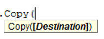 The Copy function works on a single cell, subset of cell or subset of rows/columns.
'Copy values and formatting from cell A1 to cell D1
Range("A1").Copy Range("D1")

'Copy 3x3 A1:C3 matrix to D1:F3 matrix - dimension must be same
Range("A1:C3").Copy Range("D1:F3")

'Copy rows 1:3 to rows 4:6
Range("A1:A3").EntireRow.Copy Range("A4")

'Copy columns A:C to columns D:F
Range("A1:C1").EntireColumn.Copy Range("D1")
The Copy function can also be executed without an argument. It then copies the Range to the Windows Clipboard for later Pasting.
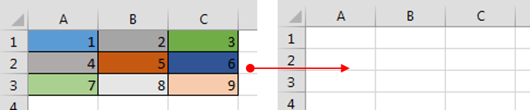
Cut function
![]() The Cut function, similarly as the Copy function, cuts single cells, ranges of cells or rows/columns.
The Cut function, similarly as the Copy function, cuts single cells, ranges of cells or rows/columns.
'Cut A1 cell and paste it to D1
Range("A1").Cut Range("D1")

'Cut 3x3 A1:C3 matrix and paste it in D1:F3 matrix - dimension must be same
Range("A1:C3").Cut Range("D1:F3")

'Cut rows 1:3 and paste to rows 4:6
Range("A1:A3").EntireRow.Cut Range("A4")

'Cut columns A:C and paste to columns D:F
Range("A1:C1").EntireColumn.Cut Range("D1")
The Cut function can be executed without arguments. It will then cut the contents of the Range and copy it to the Windows Clipboard for pasting.
Cutting cells/rows/columns does not shift any remaining cells/rows/columns but simply leaves the cut out cells empty
PasteSpecial function
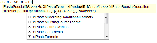 The Range PasteSpecial function works only when preceded with either the Copy or Cut Range functions. It pastes the Range (or other data) within the Clipboard to the Range on which it was executed.
Syntax
The PasteSpecial function has the following syntax:
PasteSpecial( Paste, Operation, SkipBlanks, Transpose)
The PasteSpecial function can only be used in tandem with the Copy function (not Cut)
Parameters
Paste
The part of the Range which is to be pasted. This parameter can have the following values:
| Parameter | Constant | Description | |
|---|---|---|---|
| xlPasteSpecialOperationAdd | 2 | Copied data will be added with the value in the destination cell. | |
| xlPasteSpecialOperationDivide | 5 | Copied data will be divided with the value in the destination cell. | |
| xlPasteSpecialOperationMultiply | 4 | Copied data will be multiplied with the value in the destination cell. | |
| xlPasteSpecialOperationNone | -4142 | No calculation will be done in the paste operation. | |
| xlPasteSpecialOperationSubtract | 3 | Copied data will be subtracted with the value in the destination cell. |
Operation
The paste operation e.g. paste all, only formatting, only values, etc. This can have one of the following values:
| Name | Constant | Description |
|---|---|---|
| xlPasteAll | -4104 | Everything will be pasted. |
| xlPasteAllExceptBorders | 7 | Everything except borders will be pasted. |
| xlPasteAllMergingConditionalFormats | 14 | Everything will be pasted and conditional formats will be merged. |
| xlPasteAllUsingSourceTheme | 13 | Everything will be pasted using the source theme. |
| xlPasteColumnWidths | 8 | Copied column width is pasted. |
| xlPasteComments | -4144 | Comments are pasted. |
| xlPasteFormats | -4122 | Copied source format is pasted. |
| xlPasteFormulas | -4123 | Formulas are pasted. |
| xlPasteFormulasAndNumberFormats | 11 | Formulas and Number formats are pasted. |
| xlPasteValidation | 6 | Validations are pasted. |
| xlPasteValues | -4163 | Values are pasted. |
| xlPasteValuesAndNumberFormats | 12 | Values and Number formats are pasted. |
SkipBlanks
If True then blanks will not be pasted.
Transpose
Transpose the Range before paste (swap rows with columns).
PasteSpecial Examples
'Cut A1 cell and paste its values to D1
Range("A1").Copy
Range("D1").PasteSpecial
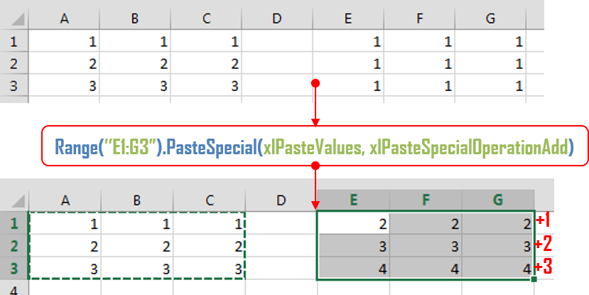
'Copy 3x3 A1:C3 matrix and add all the values to E1:G3 matrix (dimension must be same)
Range("A1:C3").Copy
Range("E1:G3").PasteSpecial xlPasteValues, xlPasteSpecialOperationAdd
Below an example where the Excel Range A1:C3 values are copied an added to the E1:G3 Range. You can also multiply, divide and run other similar operations.
Paste
The Paste function allows you to paste data in the Clipboard to the actively selected Range. Cutting and Pasting can only be accomplished with the Paste function.
'Cut A1 cell and paste its values to D1
Range("A1").Cut
Range("D1").Select
ActiveSheet.Paste

'Cut 3x3 A1:C3 matrix and paste it in D1:F3 matrix - dimension must be same
Range("A1:C3").Cut
Range("D1:F3").Select
ActiveSheet.Paste

'Cut rows 1:3 and paste to rows 4:6
Range("A1:A3").EntireRow.Cut
Range("A4").Select
ActiveSheet.Paste

'Cut columns A:C and paste to columns D:F
Range("A1:C1").EntireColumn.Cut
Range("D1").Select
ActiveSheet.Paste
Range Clear/Delete
The Clear function
The Clear function clears the entire content and formatting from an Excel Range. It does not, however, shift (delete) the cleared cells.
Range("A1:C3").Clear
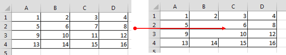
The Delete function
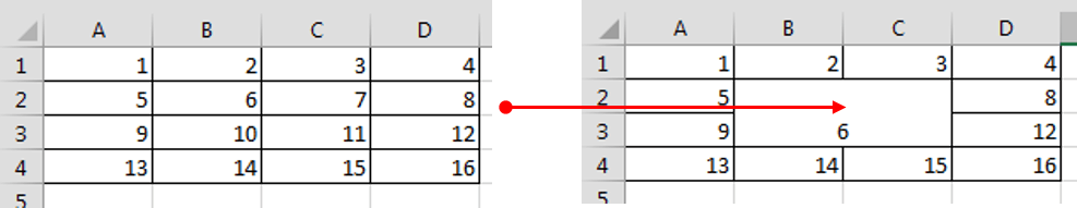
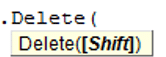 The Delete function deletes a Range of cells, removing them entirely from the Worksheet, and shifts the remaining Cells in a selected shift direction.
Although the manual Delete cell function provides 4 ways of shifting cells. The VBA Delete Shift values can only be either be xlShiftToLeft or xlShiftUp.
'If Shift omitted, Excel decides - shift up in this case
Range("B2").Delete

'Delete and Shift remaining cells left
Range("B2").Delete xlShiftToLeft

'Delete and Shift remaining cells up
Range("B2").Delete xlShiftTop

'Delete entire row 2 and shift up
Range("B2").EntireRow.Delete

'Delete entire column B and shift left
Range("B2").EntireRow.Delete
Traversing Ranges
Traversing cells is really useful when you want to run an operation on each cell within an Excel Range. Fortunately this is easily achieved in VBA using the For Each or For loops.
Dim cellRange As Range

For Each cellRange In Range("A1:C3")
  Debug.Print cellRange.Value
Next cellRange
Although this may not be obvious, beware of iterating/traversing the Excel Range using a simple For loop. For loops are not efficient on Ranges. Use a For Each loop as shown above. This is because Ranges resemble more Collections than Arrays. Read more on For vs For Each loops here
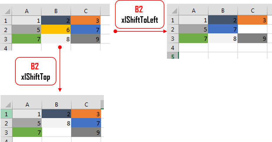
Traversing the UsedRange
 Every Worksheet has a UsedRange. This represents that smallest rectangle Range that contains all cells that have or had at some point values. In other words if the further out in the bottom, right-corner of the Worksheet there is a certain cell (e.g. E8) then the UsedRange will be as large as to include that cell starting at cell A1 (e.g. A1:E8). In Excel you can check the current UsedRange hitting CTRL+END. In VBA you get the UsedRange like this:
ActiveSheet.UsedRange
'same as
UsedRange
You can traverse through the UsedRange like this:
Dim cellRange As Range

For Each cellRange In UsedRange
  Debug.Print "Row: " & cellRange.Row & ", Column: " & cellRange.Column
Next cellRange
The UsedRange is a useful construct responsible often for bloated Excel Workbooks. Often delete unused Rows and Columns that are considered to be within the UsedRange can result in significantly reducing your file size. Read also more on the XSLB file format here
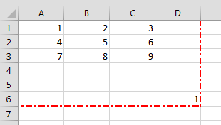
Range Addresses
The Excel Range Address property provides a string value representing the Address of the Range.
![]()
Syntax
Below the syntax of the Excel Range Address property:
Address( [RowAbsolute], [ColumnAbsolute], [ReferenceStyle], [External], [RelativeTo] )
Parameters
RowAbsolute
Optional. If True returns the row part of the reference address as an absolute reference. By default this is True.
$D$10:$G$100 'RowAbsolute is set to True
$D10:$G100 'RowAbsolute is set to False
ColumnAbsolute
Optional. If True returns the column part of the reference as an absolute reference. By default this is True.
$D$10:$G$100 'ColumnAbsolute is set to True
D$10:G$100 'ColumnAbsolute is set to False
ReferenceStyle
Optional. The reference style. The default value is xlA1. Possible values:
| Constant | Value | Description |
|---|---|---|
| xlA1 | 1 | Default. Use xlA1 to return an A1-style reference |
| xlR1C1 | -4150 | Use xlR1C1 to return an R1C1-style reference |
External
Optional. If True then property will return an external reference address, otherwise a local reference address will be returned. By default this is False.
$A$1 'Local
[Book1.xlsb]Sheet1!$A$1 'External
RelativeTo
Provided RowAbsolute and ColumnAbsolute are set to False, and the ReferenceStyle is set to xlR1C1, then you must include a starting point for the relative reference. This must be a Range variable to be set as the reference point.
Merged Ranges
![]() Merged cells are Ranges that consist of 2 or more adjacent cells. To Merge a collection of adjacent cells run Merge function on that Range.
Merged cells are Ranges that consist of 2 or more adjacent cells. To Merge a collection of adjacent cells run Merge function on that Range.
The Merge has only a single parameter – Across, a boolean which if True will merge cells in each row of the specified range as separate merged cells. Otherwise the whole Range will be merged. The default value is False.
Merge examples
To merge the entire Range:
'This will turn of any alerts warning that values may be lost
Application.DisplayAlerts = False

Range("B2:C3").Merge
This will result in the following:
To merge just the rows set Across to True.
'This will turn of any alerts warning that values may be lost
Application.DisplayAlerts = False

Range("B2:C3").Merge True
This will result in the following:
Remember that merged Ranges can only have a single value and formula. Hence, if you merge a group of cells with more than a single value/formula only the first value/formula will be set as the value/formula for your new merged Range
Checking if Range is merged
To check if a certain Range is merged simply use the Excel Range MergeCells property:
Range("B2:C3").Merge

Debug.Print Range("B2").MergeCells 'Result: True
The MergeArea
The MergeArea is a property of an Excel Range that represent the whole merge Range associated with the current Range. Say that $B$2:$C$3 is a merged Range – each cell within that Range (e.g. B2, C3..) will have the exact same MergedArea. See example below:
Range("B2:C3").Merge
Debug.Print Range("B2").MergeArea.Address 'Result: $B$2:$C$3
Named Ranges
Named Ranges are Ranges associated with a certain Name (string). In Excel you can find all your Named Ranges by going to Formulas->Name Manager. They are very useful when working on certain values that are used frequently through out your Workbook. Imagine that you are writing a Financial Analysis and want to use a common Discount Rate across all formulas. Just the address of the cell e.g. “A2”, won’t be self-explanatory. Why not use e.g. “DiscountRate” instead? Well you can do just that.
Creating a Named Range
Named Ranges can be created either within the scope of a Workbook or Worksheet:
Dim r as Range
'Within Workbook
Set r = ActiveWorkbook.Names.Add("NewName", Range("A1"))
'Within Worksheet
Set r = ActiveSheet.Names.Add("NewName", Range("A1"))
This gives you flexibility to use similar names across multiple Worksheets or use a single global name across the entire Workbook.
Listing all Named Ranges
You can list all Named Ranges using the Name Excel data type. Names are objects that represent a single NamedRange. See an example below of listing our two newly created NamedRanges:
Call ActiveWorkbook.Names.Add("NewName", Range("A1"))
Call ActiveSheet.Names.Add("NewName", Range("A1"))

Dim n As Name
For Each n In ActiveWorkbook.Names
  Debug.Print "Name: " & n.Name & ", Address: " & _
       n.RefersToRange.Address & ", Value: "; n.RefersToRange.Value
Next n

'Result:
'Name: Sheet1!NewName, Address: $A$1, Value:  1
'Name: NewName, Address: $A$1, Value:  1
SpecialCells
SpecialCells are a very useful Excel Range property, that allows you to select a subset of cells/Ranges within a certain Range.
Syntax
The SpecialCells property has the following syntax:
SpecialCells( Type, [Value] )
Parameters
Type
The type of cells to be returned. Possible values:
| Constant | Value | Description |
|---|---|---|
| xlCellTypeAllFormatConditions | -4172 | Cells of any format |
| xlCellTypeAllValidation | -4174 | Cells having validation criteria |
| xlCellTypeBlanks | 4 | Empty cells |
| xlCellTypeComments | -4144 | Cells containing notes |
| xlCellTypeConstants | 2 | Cells containing constants |
| xlCellTypeFormulas | -4123 | Cells containing formulas |
| xlCellTypeLastCell | 11 | The last cell in the used range |
| xlCellTypeSameFormatConditions | -4173 | Cells having the same format |
| xlCellTypeSameValidation | -4175 | Cells having the same validation criteria |
| xlCellTypeVisible | 12 | All visible cells |
Value
If Type is equal to xlCellTypeConstants or xlCellTypeFormulas this determines the types of cells to return e.g. with errors.
| Constant | Value |
|---|---|
| xlErrors | 16 |
| xlLogical | 4 |
| xlNumbers | 1 |
| xlTextValues | 2 |
SpecialCells examples
Get Excel Range with Constants
This will return only cells with constant cells within the Range C1:C3:
For Each r In Range("A1:C3").SpecialCells(xlCellTypeConstants)
  Debug.Print r.Value
Next r
Search for Excel Range with Errors
For Each r In ActiveSheet.UsedRange.SpecialCells(xlCellTypeFormulas, xlErrors)
  Debug.Print r.Address
Next r