
О чём пойдёт речь?
Знакомство с объектной моделью Excel следует начинать с такого замечательного объекта, как Range. Поскольку любая ячейка — это Range, то без знания, как с этим объектом эффективно взаимодействовать, вам будет затруднительно программировать для Excel. Это очень ладно-скроенный объект. При некоторой сноровке вы найдёте его весьма удобным в эксплуатации.
Что такое объекты?
Мы собираемся изучать объект Range, поэтому пару слов надо сказать, что такое, собственно, «объект«. Всё, что вы наблюдаете в Excel, всё с чем вы работаете — это набор объектов. Например, лист рабочей книги Excel — не что иное, как объект типа WorkSheet. Однотипные объекты объединяют в коллекции себе подобных. Например, листы объединены в коллекцию Sheets. Чтобы не путать друг с другом объекты одного и того же типа, они имеют отличающиеся имена, а также номер индекса в коллекции. Объекты имеют свойства, методы и события.
Свойства — это информация об объекте. Часто эти свойства можно менять, что автоматически влечет изменения внешнего вида объекта или его поведения. Например свойство Visible объекта Worksheet отвечает за видимость листа на экране. Если ему присвоить значение xlSheetHidden (это константа, которая по факту равно нулю), то лист будет скрыт.
Методы — это то, что объект может делать. Например, метод Delete объекта Worksheet удаляет себя из книги. Метод Select делает лист активным.
События — это механизм, при помощи которого вы можете исполнять свой код VBA сразу по факту возникновения того или иного события с вашим объектом. Например, есть возможность выполнять ваш код, как только пользователь сделал текущим определенный лист рабочей книги, либо как только пользователь что-то изменил на этом листе.
Range это диапазон ячеек. Минимум — одна ячейка, максимум — весь лист, теоретически насчитывающий более 17 миллиардов ячеек (строки 2^20 * столбцы 2^14 = 2^34).
В Excel объявлены глобально и всегда готовы к использованию несколько коллекций, имеющий членами объекты типа Range, либо свойства это же типа.
Коллекции глобального объекта Application: Cells, Columns, Rows, а также свойства Range, Selection, ActiveCell, ThisCell.
ActiveCell — активная ячейка текущего листа, ThisCell — если вы написали пользовательскую функцию рабочего листа, то через это свойство вы можете определить какая конкретно ячейка в данный момент пересчитывает вашу функцию. Об остальных перечисленных объектов речь пойдёт ниже.
Работа с отдельными ячейками
| Синтаксическая форма | Комментарии по использованию |
| Range(«D5«) или [D5] |
Ячейка D5 текущего листа. Полная и краткая формы. Тут применим только синтаксис типа A1, но не R1C1. То есть такая конструкция Range(«R1C2«) — вызовет ошибку, даже если в книге Excel включен режим формул R1C1. Разумеется после этой формы вы можете обратиться к свойствам соответствующей ячейки. Например, Range(«D5«).Interior.Color = RGB(0, 255, 0). |
| Cells(5, 4) или Cells(5, «D») | Ячейка D5 текущего листа через свойство Cells. 5 — строка (row), 4 — столбец (column). Допустимость второй формы мало кому известна. |
| Cells(65540) | Ячейку D5 можно адресовать и через указание только одного параметра свойсва Cells. При этом нумерация идёт слева направо, потом сверху вниз. То есть сначала нумеруется вся строка (2^14=16384 колонок) и только потом идёт переход на следующую строку. То есть Cells(16385) вернёт вам ячейку A2, а D5 будет Cells(65540). Пока данный способ выглядит не очень удобным. |
Работа с диапазоном ячеек
| Синтаксическая форма | Комментарии по использованию |
| Range(«A1:B4«) или [A1:B4] | Диапазон ячеек A1:B4 текущего листа. Обратите внимание, что указываются координаты верхнего левого и правого нижнего углов диапазона. Причём первый указываемый угол вполне может быть правым нижним, это не имеет значения. |
| Range(Cells(1, 1), Cells(4, 2)) | Диапазон ячеек A1:B4 текущего листа. Удобно, когда вы знаете именно цифровые координаты углов диапазона. |
Работа со строками
| Синтаксическая форма | Комментарии по использованию |
| Range(«3:5«) или [3:5] | Строки 3, 4 и 5 текущего листа целиком. |
| Range(«A3:XFD3«) или [A3:XFD3] | Строка 3, но с указанием колонок. Просто, чтобы вы понимали, что это тождественные формы. XFD — последняя колонка листа. |
| Rows(«3:3«) | Строка 3 через свойство Rows. Параметр в виде диапазона строк. Двоеточие — это символ диапазона. |
| Rows(3) | Тут параметр — индекс строки в массиве строк. Так можно сослаться только не конкретную строку. Обратите внимание, что в предыдущем примере параметр текстовая строка «3:3» и она взята в кавычки, а тут — чистое число. |
Работа со столбцами
| Синтаксическая форма | Комментарии по использованию |
| Range(«B:B«) или [B:B] | Колонка B текущего листа. |
| Range(«B1:B1048576«) или [B1:B1048576] | То же самое, но с указанием номеров строк, чтобы вы понимали, что это тождественные формы. 2^20=1048576 — максимальный номер строки на листе. |
| Columns(«B:B«) | То же самое через свойство Columns. Параметр — текстовая строка. |
| Columns(2) | То же самое. Параметр — числовой индекс столбца. «A» -> 1, «B» -> 2, и т.д. |
Весь лист
| Синтаксическая форма | Комментарии по использованию |
| Range(«A1:XFD1048576«) или [A1:XFD1048576] | Диапазон размером во всё адресное пространство листа Excel. Воспринимайте эту таблицу лишь как теорию — так работать с листами вам не придётся — слишком большое количество ячеек. Даже современные компьютеры не смогут помочь Excel быстро работать с такими массивами информации. Тут проблема больше даже в самом приложении. |
| Range(«1:1048576«) или [1:1048576] | То же самое, но через строки. |
| Range(«A:XFD«) или [A:XFD] | Аналогично — через адреса столбцов. |
| Cells | Свойство Cells включает в себя ВСЕ ячейки. |
| Rows | Все строки листа. |
| Columns | Все столбцы листа. |
Следует иметь в виду, что свойства Range, Cells, Columns и Rows имеют как объекты типа Worksheet, так и объекты Range. Соответственно в первом случае эти коллекции будут относиться ко всему листу и отсчитываться будут от A1, а вот в случае конкретного объекта Range эти коллекции будут относиться только к ячейкам этого диапазона и отсчитываться будут от левого верхнего угла диапазона. Например Cells(2,2) указывает на ячейку B2, а Range(«C3:D5»).Cells(2,2) укажет на D4.
Также много путаницы в умы вносит тот факт, что объект Range имеет одноименное свойство range. К примеру, Range(«A100:D500»).Range(«A2») — тут выражение до точки ( Range(«A100:D500») ) является объектом Range, выражение после точки ( Range(«A2») ) — свойство range упомянутого объекта, но возвращает это свойство тоже объект типа Range. Вот такие пироги. Из этого следует, что такая цепочка может иметь и более двух членов. Практического смысла в этом будет не много, но синтаксически это будут совершенно корректно, например, так: Range(«CV100:GR200»).Range(«J10:T20»).Range(«A1:B2») укажет на диапазон DE109:DF110.
Ещё один сюрприз таится в том, что объекты Range имеют свойство по-умолчанию Item( RowIndex [, ColumnIndex] ). По правилам VBA при ссылке на default свойства имя свойства (Item) можно опускать. Кстати говоря, то что вы привыкли видеть в скобках после Cells, есть не что иное, как это дефолтовое свойство Item, а не родные параметры Cells, который их не имеет вовсе. Ну ладно к Cells все привыкли и это никакого отторжения не вызывает, но если вы увидите нечто подобное — Range(«C3:D5»)(2,2), то, скорее всего, будете несколько озадачены, а тем временем — это буквально тоже самое, что и у Cells — всё то же дефолтовое свойство Item. Последняя конструкция ссылается на D4. А вот для Columns и Rows свойство Item может быть только одночленным, например Columns(1) — и к этой форме мы тоже вполне привыкли. Однако конструкции вида Columns(2)(3)(4) могут сильно удивить (столбец 7 будет выделен).
Примеры кода
Скачать
Типовые задачи
-
Перебор ячеек в диапазоне (вариант 1)
В данном примере организован цикл For…Next и доступ к ячейкам осуществляется по их индексу. Вместо parRange(i) мы могли бы написать parRange.Item(i) (выше это объяснялось). Обратите внимание, что мы в этом примере успешно применяем, как вариант с parRange(i,c), так и parRange(i). То есть, если мы применяем одночленную форму свойства Item, то диапазон перебирается по строкам (A1, B1, C1, A2, …), а если двухчленную, то столбец у нас зафиксирован и каждая итерация цикла — на новой строке. Это очень интересный эффект, его можно применять для вытягивания таблиц по вертикали. Но — продолжим!
Количество ячеек в диапазоне получено при помощи свойства .Count. Как .Item, так и .Count — это всё атрибуты коллекций, которые широко применяются в объектой модели MS Office и, в частности, Excel.
Sub Handle_Cells_1(parRange As Range)
  For i = 1 To parRange.Count
    parRange(i, 5) = parRange(i).Address & " = " & parRange(i)
  Next
End Sub
-
Перебор ячеек в диапазоне (вариант 2)
В этом примере мы использовали цикл For each…Next, что выглядит несколько лаконичней. Однако, в некоторых случаях вам может потребоваться переменная i из предыдущего примера, например, для вывода результатов в определенные строки листа, поэтому выбирайте удробную вам форму оператора For. Тут в цикле мы «вытягивали» все ячейки диапазона в текстовую строку, чтобы потом отобразить её через функцию MsgBox.
Sub Handle_Cells_2(parRange As Range)
  For Each c In parRange
    strLine = strLine & c.Address & "=" & c & "; "
  Next
  MsgBox strLine
End Sub
-
Перебор ячеек в диапазоне (вариант 3)
Если необходимо перебирать ячейки в порядке A1, A2, A3, B1, …, а не A1, B1, C1, A2, …, то вы можете это организовать при помощи 2-х циклов For. Обратите внимание, как мы узнали количество столбцов (parRange.Columns.Count) и строк (parRange.Rows.Count) в диапазоне, а также на использование свойства Cells. Тут Cells относится к листу и никак не связано с диапазоном parRange.
Sub Handle_Cells_3(parRange As Range)
  colNum = parRange.Columns.Count
  For i = 1 To parRange.Rows.Count
    For j = 1 To colNum
      Cells(i + (j - 1) * colNum, colNum + 2) = parRange(i, j)
    Next j
  Next i
End Sub
-
Перебор строк диапазона
В цикле For each…Next перебираем коллекцию Rows объекта parRange. Для каждой строки формируем цвет на основе первых трёх ячеек каждой строки. Поскульку у нас в ячейках формула, присваивающая ячейке случайное число от 1 до 255, то цвета получаются всегда разные. Оператор With позволяет нам сократить код и, к примеру, вместо Line.Cells(2) написать просто .Cells(2).
Sub Handle_Rows_1(parRange As Range)
  For Each Line In parRange.Rows
    With Line
      .Interior.Color = RGB(.Cells(1), .Cells(2), .Cells(3))
    End With
  Next
End Sub
-
Перебор столбцов
Перебираем коллекцию Columns. Тоже используем оператор With. В последней ячейке каждого столбца у нас хранится размер шрифта для всей колонки, который мы и применяем к свойству Line.Font.Size.
Sub Handle_Columns_1(parRange As Range)
  For Each Line In parRange.Columns
    With Line
      .Font.Size = .Cells(.Cells.Count)
    End With
  Next
End Sub
-
Перебор областей диапазона
Как вы знаете, в Excel можно выделить несвязанные диапазоны и проделать с ними какие-то операции. Поддерживает это и объект Range. Получить диапазон, состоящий из нескольких областей (area) очень легко — достаточно перечислить через запятую адреса соответствующих диапазонов: Range(«A1:B3, B5:D8, Z1:AA12«).
Вот такой составной диапазон и разбирается процедурой, показанной ниже. Организован цикл по коллекции Areas, настроен оператор with на текущий элемент коллекции, и ниже и правее относительно ячейки J1 мы собираем некоторые сведения о свойствах областей составного диапазона (которые каждый по себе, конечно же, тоже являются объектами типа Range). Для задания смещения от ячейки J1 нами впервые использовано очень полезное свойство Offset. Каждый диапазон получает случайный цвет, плюс мы заносим в таблицу порядковый номер диапазона (i), его адрес (.Address), количество ячеек (.Count) и цвет (.Interior.Color) после того, как он вычислен.Sub Handle_Areas_1(parRange As Range) For i = 1 To parRange.Areas.Count With parRange.Areas(i) Cells(1, 10).Offset(i, 0) = i Cells(1, 10).Offset(i, 1) = .Address Cells(1, 10).Offset(i, 2) = .Count .Interior.Color = RGB(Int(Rnd * 255), Int(Rnd * 255), Int(Rnd * 255)) Cells(1, 10).Offset(i, 3) = .Interior.Color End With Next End Sub
Продолжение следует…
Читайте также:
-
Поиск границ текущей области
-
Массивы в VBA
-
Структуры данных и их эффективность
-
Автоматическое скрытие/показ столбцов и строк
Свойства ячейки, часто используемые в коде VBA Excel. Демонстрация свойств ячейки, как структурной единицы объекта Range, на простых примерах.
Объект Range в VBA Excel представляет диапазон ячеек. Он (объект Range) может описывать любой диапазон, начиная от одной ячейки и заканчивая сразу всеми ячейками рабочего листа.
Примеры диапазонов:
- Одна ячейка –
Range("A1"). - Девять ячеек –
Range("A1:С3"). - Весь рабочий лист в Excel 2016 –
Range("1:1048576").
Для справки: выражение Range("1:1048576") описывает диапазон с 1 по 1048576 строку, где число 1048576 – это номер последней строки на рабочем листе Excel 2016.
В VBA Excel есть свойство Cells объекта Range, которое позволяет обратиться к одной ячейке в указанном диапазоне (возвращает объект Range в виде одной ячейки). Если в коде используется свойство Cells без указания диапазона, значит оно относится ко всему диапазону активного рабочего листа.
Примеры обращения к одной ячейке:
Cells(1000), где 1000 – порядковый номер ячейки на рабочем листе, возвращает ячейку «ALL1».Cells(50, 20), где 50 – номер строки рабочего листа, а 20 – номер столбца, возвращает ячейку «T50».Range("A1:C3").Cells(6), где «A1:C3» – заданный диапазон, а 6 – порядковый номер ячейки в этом диапазоне, возвращает ячейку «C2».
Для справки: порядковый номер ячейки в диапазоне считается построчно слева направо с перемещением к следующей строке сверху вниз.
Подробнее о том, как обратиться к ячейке, смотрите в статье: Ячейки (обращение, запись, чтение, очистка).
В этой статье мы рассмотрим свойства объекта Range, применимые, в том числе, к диапазону, состоящему из одной ячейки.
Еще надо добавить, что свойства и методы объектов отделяются от объектов точкой, как в третьем примере обращения к одной ячейке: Range("A1:C3").Cells(6).
Свойства ячейки (объекта Range)
| Свойство | Описание |
|---|---|
| Address | Возвращает адрес ячейки (диапазона). |
| Borders | Возвращает коллекцию Borders, представляющую границы ячейки (диапазона). Подробнее… |
| Cells | Возвращает объект Range, представляющий коллекцию всех ячеек заданного диапазона. Указав номер строки и номер столбца или порядковый номер ячейки в диапазоне, мы получаем конкретную ячейку. Подробнее… |
| Characters | Возвращает подстроку в размере указанного количества символов из текста, содержащегося в ячейке. Подробнее… |
| Column | Возвращает номер столбца ячейки (первого столбца диапазона). Подробнее… |
| ColumnWidth | Возвращает или задает ширину ячейки в пунктах (ширину всех столбцов в указанном диапазоне). |
| Comment | Возвращает комментарий, связанный с ячейкой (с левой верхней ячейкой диапазона). |
| CurrentRegion | Возвращает прямоугольный диапазон, ограниченный пустыми строками и столбцами. Очень полезное свойство для возвращения рабочей таблицы, а также определения номера последней заполненной строки. |
| EntireColumn | Возвращает весь столбец (столбцы), в котором содержится ячейка (диапазон). Диапазон может содержаться и в одном столбце, например, Range("A1:A20"). |
| EntireRow | Возвращает всю строку (строки), в которой содержится ячейка (диапазон). Диапазон может содержаться и в одной строке, например, Range("A2:H2"). |
| Font | Возвращает объект Font, представляющий шрифт указанного объекта. Подробнее о цвете шрифта… |
| HorizontalAlignment | Возвращает или задает значение горизонтального выравнивания содержимого ячейки (диапазона). Подробнее… |
| Interior | Возвращает объект Interior, представляющий внутреннюю область ячейки (диапазона). Применяется, главным образом, для возвращения или назначения цвета заливки (фона) ячейки (диапазона). Подробнее… |
| Name | Возвращает или задает имя ячейки (диапазона). |
| NumberFormat | Возвращает или задает код числового формата для ячейки (диапазона). Примеры кодов числовых форматов можно посмотреть, открыв для любой ячейки на рабочем листе Excel диалоговое окно «Формат ячеек», на вкладке «(все форматы)». Свойство NumberFormat диапазона возвращает значение NULL, за исключением тех случаев, когда все ячейки в диапазоне имеют одинаковый числовой формат. Если нужно присвоить ячейке текстовый формат, записывается так: Range("A1").NumberFormat = "@". Общий формат: Range("A1").NumberFormat = "General". |
| Offset | Возвращает объект Range, смещенный относительно первоначального диапазона на указанное количество строк и столбцов. Подробнее… |
| Resize | Изменяет размер первоначального диапазона до указанного количества строк и столбцов. Строки добавляются или удаляются снизу, столбцы – справа. Подробнее… |
| Row | Возвращает номер строки ячейки (первой строки диапазона). Подробнее… |
| RowHeight | Возвращает или задает высоту ячейки в пунктах (высоту всех строк в указанном диапазоне). |
| Text | Возвращает форматированный текст, содержащийся в ячейке. Свойство Text диапазона возвращает значение NULL, за исключением тех случаев, когда все ячейки в диапазоне имеют одинаковое содержимое и один формат. Предназначено только для чтения. Подробнее… |
| Value | Возвращает или задает значение ячейки, в том числе с отображением значений в формате Currency и Date. Тип данных Variant. Value является свойством ячейки по умолчанию, поэтому в коде его можно не указывать. |
| Value2 | Возвращает или задает значение ячейки. Тип данных Variant. Значения в формате Currency и Date будут отображены в виде чисел с типом данных Double. |
| VerticalAlignment | Возвращает или задает значение вертикального выравнивания содержимого ячейки (диапазона). Подробнее… |
В таблице представлены не все свойства объекта Range. С полным списком вы можете ознакомиться не сайте разработчика.
Простые примеры для начинающих
Вы можете скопировать примеры кода VBA Excel в стандартный модуль и запустить их на выполнение. Как создать стандартный модуль и запустить процедуру на выполнение, смотрите в статье VBA Excel. Начинаем программировать с нуля.
Учтите, что в одном программном модуле у всех процедур должны быть разные имена. Если вы уже копировали в модуль подпрограммы с именами Primer1, Primer2 и т.д., удалите их или создайте еще один стандартный модуль.
Форматирование ячеек
Заливка ячейки фоном, изменение высоты строки, запись в ячейки текста, автоподбор ширины столбца, выравнивание текста в ячейке и выделение его цветом, добавление границ к ячейкам, очистка содержимого и форматирования ячеек.
Если вы запустите эту процедуру, информационное окно MsgBox будет прерывать выполнение программы и сообщать о том, что произойдет дальше, после его закрытия.
|
1 2 3 4 5 6 7 8 9 10 11 12 13 14 15 16 17 18 19 20 21 22 23 24 25 26 27 28 29 30 31 32 33 34 35 36 37 38 |
Sub Primer1() MsgBox «Зальем ячейку A1 зеленым цветом и запишем в ячейку B1 текст: «Ячейка A1 зеленая!»» Range(«A1»).Interior.Color = vbGreen Range(«B1»).Value = «Ячейка A1 зеленая!» MsgBox «Сделаем высоту строки, в которой находится ячейка A2, в 2 раза больше высоты ячейки A1, « _ & «а в ячейку B1 вставим текст: «Наша строка стала в 2 раза выше первой строки!»» Range(«A2»).RowHeight = Range(«A1»).RowHeight * 2 Range(«B2»).Value = «Наша строка стала в 2 раза выше первой строки!» MsgBox «Запишем в ячейку A3 высоту 2 строки, а в ячейку B3 вставим текст: «Такова высота второй строки!»» Range(«A3»).Value = Range(«A2»).RowHeight Range(«B3»).Value = «Такова высота второй строки!» MsgBox «Применим к столбцу, в котором содержится ячейка B1, метод AutoFit для автоподбора ширины» Range(«B1»).EntireColumn.AutoFit MsgBox «Выделим текст в ячейке B2 красным цветом и выровним его по центру (по вертикали)» Range(«B2»).Font.Color = vbRed Range(«B2»).VerticalAlignment = xlCenter MsgBox «Добавим к ячейкам диапазона A1:B3 границы» Range(«A1:B3»).Borders.LineStyle = True MsgBox «Сделаем границы ячеек в диапазоне A1:B3 двойными» Range(«A1:B3»).Borders.LineStyle = xlDouble MsgBox «Очистим ячейки диапазона A1:B3 от заливки, выравнивания, границ и содержимого» Range(«A1:B3»).Clear MsgBox «Присвоим высоте второй строки высоту первой, а ширине второго столбца — ширину первого» Range(«A2»).RowHeight = Range(«A1»).RowHeight Range(«B1»).ColumnWidth = Range(«A1»).ColumnWidth MsgBox «Демонстрация форматирования ячеек закончена!» End Sub |
Вычисления в ячейках (свойство Value)
Запись двух чисел в ячейки, вычисление их произведения, вставка в ячейку формулы, очистка ячеек.
Обратите внимание, что разделителем дробной части у чисел в VBA Excel является точка, а не запятая.
|
1 2 3 4 5 6 7 8 9 10 11 12 13 14 15 16 17 18 19 20 21 22 23 24 |
Sub Primer2() MsgBox «Запишем в ячейку A1 число 25.3, а в ячейку B1 — число 34.42» Range(«A1»).Value = 25.3 Range(«B1»).Value = 34.42 MsgBox «Запишем в ячейку C1 произведение чисел, содержащихся в ячейках A1 и B1» Range(«C1»).Value = Range(«A1»).Value * Range(«B1»).Value MsgBox «Запишем в ячейку D1 формулу, которая перемножает числа в ячейках A1 и B1» Range(«D1»).Value = «=A1*B1» MsgBox «Заменим содержимое ячеек A1 и B1 на числа 6.258 и 54.1, а также активируем ячейку D1» Range(«A1»).Value = 6.258 Range(«B1»).Value = 54.1 Range(«D1»).Activate MsgBox «Мы видим, что в ячейке D1 произведение изменилось, а в строке состояния отображается формула; « _ & «следующим шагом очищаем задействованные ячейки» Range(«A1:D1»).Clear MsgBox «Демонстрация вычислений в ячейках завершена!» End Sub |
Так как свойство Value является свойством ячейки по умолчанию, его можно было нигде не указывать. Попробуйте удалить .Value из всех строк, где оно встречается и запустить код заново.
Различие свойств Text, Value и Value2
Построение с помощью кода VBA Excel таблицы с результатами сравнения того, как свойства Text, Value и Value2 возвращают число, дату и текст.
|
1 2 3 4 5 6 7 8 9 10 11 12 13 14 15 16 17 18 19 20 21 22 23 24 25 26 27 28 29 30 31 32 33 34 35 36 37 38 39 40 41 42 43 44 45 46 47 48 49 50 51 52 53 54 55 56 |
Sub Primer3() ‘Присваиваем ячейкам всей таблицы общий формат на тот ‘случай, если формат отдельных ячеек ранее менялся Range(«A1:E4»).NumberFormat = «General» ‘добавляем сетку (границы ячеек) Range(«A1:E4»).Borders.LineStyle = True ‘Создаем строку заголовков Range(«A1») = «Значение» Range(«B1») = «Код формата» ‘формат соседней ячейки в столбце A Range(«C1») = «Свойство Text» Range(«D1») = «Свойство Value» Range(«E1») = «Свойство Value2» ‘Назначаем строке заголовков жирный шрифт Range(«A1:E1»).Font.Bold = True ‘Задаем форматы ячейкам A2, A3 и A4 ‘Ячейка A2 — числовой формат с разделителем триад и двумя знаками после запятой ‘Ячейка A3 — формат даты «ДД.ММ.ГГГГ» ‘Ячейка A4 — текстовый формат Range(«A2»).NumberFormat = «# ##0.00» Range(«A3»).NumberFormat = «dd.mm.yyyy» Range(«A4»).NumberFormat = «@» ‘Заполняем ячейки A2, A3 и A4 значениями Range(«A2») = 2362.4568 Range(«A3») = CDate(«01.01.2021») ‘Функция CDate преобразует текстовый аргумент в формат даты Range(«A4») = «Озеро Байкал» ‘Заполняем ячейки B2, B3 и B4 кодами форматов соседних ячеек в столбце A Range(«B2») = Range(«A2»).NumberFormat Range(«B3») = Range(«A3»).NumberFormat Range(«B4») = Range(«A4»).NumberFormat ‘Присваиваем ячейкам C2-C4 значения свойств Text ячеек A2-A4 Range(«C2») = Range(«A2»).Text Range(«C3») = Range(«A3»).Text Range(«C4») = Range(«A4»).Text ‘Присваиваем ячейкам D2-D4 значения свойств Value ячеек A2-A4 Range(«D2») = Range(«A2»).Value Range(«D3») = Range(«A3»).Value Range(«D4») = Range(«A4»).Value ‘Присваиваем ячейкам E2-E4 значения свойств Value2 ячеек A2-A4 Range(«E2») = Range(«A2»).Value2 Range(«E3») = Range(«A3»).Value2 Range(«E4») = Range(«A4»).Value2 ‘Применяем к таблице автоподбор ширины столбцов Range(«A1:E4»).EntireColumn.AutoFit End Sub |
Результат работы кода:

В таблице наглядно видна разница между свойствами Text, Value и Value2 при применении их к ячейкам с отформатированным числом и датой. Свойство Text еще отличается от Value и Value2 тем, что оно предназначено только для чтения.
На чтение 18 мин. Просмотров 75k.

сэр Артур Конан Дойл
Это большая ошибка — теоретизировать, прежде чем кто-то получит данные
Эта статья охватывает все, что вам нужно знать об использовании ячеек и диапазонов в VBA. Вы можете прочитать его от начала до конца, так как он сложен в логическом порядке. Или использовать оглавление ниже, чтобы перейти к разделу по вашему выбору.
Рассматриваемые темы включают свойство смещения, чтение
значений между ячейками, чтение значений в массивы и форматирование ячеек.
Содержание
- Краткое руководство по диапазонам и клеткам
- Введение
- Важное замечание
- Свойство Range
- Свойство Cells рабочего листа
- Использование Cells и Range вместе
- Свойство Offset диапазона
- Использование диапазона CurrentRegion
- Использование Rows и Columns в качестве Ranges
- Использование Range вместо Worksheet
- Чтение значений из одной ячейки в другую
- Использование метода Range.Resize
- Чтение Value в переменные
- Как копировать и вставлять ячейки
- Чтение диапазона ячеек в массив
- Пройти через все клетки в диапазоне
- Форматирование ячеек
- Основные моменты
Краткое руководство по диапазонам и клеткам
| Функция | Принимает | Возвращает | Пример | Вид |
| Range | адреса ячеек |
диапазон ячеек |
.Range(«A1:A4») | $A$1:$A$4 |
| Cells | строка, столбец |
одна ячейка |
.Cells(1,5) | $E$1 |
| Offset | строка, столбец |
диапазон | .Range(«A1:A2») .Offset(1,2) |
$C$2:$C$3 |
| Rows | строка (-и) | одна или несколько строк |
.Rows(4) .Rows(«2:4») |
$4:$4 $2:$4 |
| Columns | столбец (-цы) |
один или несколько столбцов |
.Columns(4) .Columns(«B:D») |
$D:$D $B:$D |
Введение
Это третья статья, посвященная трем основным элементам VBA. Этими тремя элементами являются Workbooks, Worksheets и Ranges/Cells. Cells, безусловно, самая важная часть Excel. Почти все, что вы делаете в Excel, начинается и заканчивается ячейками.
Вы делаете три основных вещи с помощью ячеек:
- Читаете из ячейки.
- Пишите в ячейку.
- Изменяете формат ячейки.
В Excel есть несколько методов для доступа к ячейкам, таких как Range, Cells и Offset. Можно запутаться, так как эти функции делают похожие операции.
В этой статье я расскажу о каждом из них, объясню, почему они вам нужны, и когда вам следует их использовать.
Давайте начнем с самого простого метода доступа к ячейкам — с помощью свойства Range рабочего листа.
Важное замечание
Я недавно обновил эту статью, сейчас использую Value2.
Вам может быть интересно, в чем разница между Value, Value2 и значением по умолчанию:
' Value2
Range("A1").Value2 = 56

' Value
Range("A1").Value = 56

' По умолчанию используется значение
Range("A1") = 56
Использование Value может усечь число, если ячейка отформатирована, как валюта. Если вы не используете какое-либо свойство, по умолчанию используется Value.
Лучше использовать Value2, поскольку он всегда будет возвращать фактическое значение ячейки.
Свойство Range
Рабочий лист имеет свойство Range, которое можно использовать для доступа к ячейкам в VBA. Свойство Range принимает тот же аргумент, что и большинство функций Excel Worksheet, например: «А1», «А3: С6» и т.д.
В следующем примере показано, как поместить значение в ячейку с помощью свойства Range.
Sub ZapisVYacheiku()

    ' Запишите число в ячейку A1 на листе 1 этой книги
    ThisWorkbook.Worksheets("Лист1").Range("A1").Value2 = 67

    ' Напишите текст в ячейку A2 на листе 1 этой рабочей книги
    ThisWorkbook.Worksheets("Лист1").Range("A2").Value2 = "Иван Петров"

    ' Запишите дату в ячейку A3 на листе 1 этой книги
    ThisWorkbook.Worksheets("Лист1").Range("A3").Value2 = #11/21/2019#

End Sub
Как видно из кода, Range является членом Worksheets, которая, в свою очередь, является членом Workbook. Иерархия такая же, как и в Excel, поэтому должно быть легко понять. Чтобы сделать что-то с Range, вы должны сначала указать рабочую книгу и рабочий лист, которому она принадлежит.
В оставшейся части этой статьи я буду использовать кодовое имя для ссылки на лист.

Следующий код показывает приведенный выше пример с использованием кодового имени рабочего листа, т.е. Лист1 вместо ThisWorkbook.Worksheets («Лист1»).
Sub IspKodImya ()

    ' Запишите число в ячейку A1 на листе 1 этой книги
     Sheet1.Range("A1").Value2 = 67

    ' Напишите текст в ячейку A2 на листе 1 этой рабочей книги
    Sheet1.Range("A2").Value2 = "Иван Петров"

    ' Запишите дату в ячейку A3 на листе 1 этой книги
    Sheet1.Range("A3").Value2 = #11/21/2019#

End Sub
Вы также можете писать в несколько ячеек, используя свойство
Range
Sub ZapisNeskol()

    ' Запишите число в диапазон ячеек
    Sheet1.Range("A1:A10").Value2 = 67

    ' Написать текст в несколько диапазонов ячеек
    Sheet1.Range("B2:B5,B7:B9").Value2 = "Иван Петров"

End Sub
Свойство Cells рабочего листа
У Объекта листа есть другое свойство, называемое Cells, которое очень похоже на Range . Есть два отличия:
- Cells возвращают диапазон только одной ячейки.
- Cells принимает строку и столбец в качестве аргументов.
В приведенном ниже примере показано, как записывать значения
в ячейки, используя свойства Range и Cells.
Sub IspCells()

    ' Написать в А1
    Sheet1.Range("A1").Value2 = 10
    Sheet1.Cells(1, 1).Value2  = 10

    ' Написать в А10
    Sheet1.Range("A10").Value2 = 10
    Sheet1.Cells(10, 1).Value2  = 10

    ' Написать в E1
    Sheet1.Range("E1").Value2 = 10
    Sheet1.Cells(1, 5).Value2  = 10

End Sub
Вам должно быть интересно, когда использовать Cells, а когда Range. Использование Range полезно для доступа к одним и тем же ячейкам при каждом запуске макроса.
Например, если вы использовали макрос для вычисления суммы и
каждый раз записывали ее в ячейку A10, тогда Range подойдет для этой задачи.
Использование свойства Cells полезно, если вы обращаетесь к
ячейке по номеру, который может отличаться. Проще объяснить это на примере.
В следующем коде мы просим пользователя указать номер столбца. Использование Cells дает нам возможность использовать переменное число для столбца.
Sub ZapisVPervuyuPustuyuYacheiku()

    Dim UserCol As Integer

    ' Получить номер столбца от пользователя
    UserCol = Application.InputBox("Пожалуйста, введите номер столбца...", Type:=1)

    ' Написать текст в выбранный пользователем столбец
    Sheet1.Cells(1, UserCol).Value2 = "Иван Петров"

End Sub
В приведенном выше примере мы используем номер для столбца,
а не букву.
Чтобы использовать Range здесь, потребуется преобразовать эти значения в ссылку на
буквенно-цифровую ячейку, например, «С1». Использование свойства Cells позволяет нам
предоставить строку и номер столбца для доступа к ячейке.
Иногда вам может понадобиться вернуть более одной ячейки, используя номера строк и столбцов. В следующем разделе показано, как это сделать.
Использование Cells и Range вместе
Как вы уже видели, вы можете получить доступ только к одной ячейке, используя свойство Cells. Если вы хотите вернуть диапазон ячеек, вы можете использовать Cells с Range следующим образом:
Sub IspCellsSRange()

    With Sheet1
        ' Запишите 5 в диапазон A1: A10, используя свойство Cells
        .Range(.Cells(1, 1), .Cells(10, 1)).Value2 = 5

        ' Диапазон B1: Z1 будет выделен жирным шрифтом
        .Range(.Cells(1, 2), .Cells(1, 26)).Font.Bold = True

    End With

End Sub
Как видите, вы предоставляете начальную и конечную ячейку
диапазона. Иногда бывает сложно увидеть, с каким диапазоном вы имеете дело,
когда значением являются все числа. Range имеет свойство Address, которое
отображает буквенно-цифровую ячейку для любого диапазона. Это может
пригодиться, когда вы впервые отлаживаете или пишете код.
В следующем примере мы распечатываем адрес используемых нами
диапазонов.
Sub PokazatAdresDiapazona()

    ' Примечание. Использование подчеркивания позволяет разделить строки кода.
    With Sheet1

        ' Запишите 5 в диапазон A1: A10, используя свойство Cells
        .Range(.Cells(1, 1), .Cells(10, 1)).Value2 = 5
        Debug.Print "Первый адрес: " _
            + .Range(.Cells(1, 1), .Cells(10, 1)).Address

        ' Диапазон B1: Z1 будет выделен жирным шрифтом
        .Range(.Cells(1, 2), .Cells(1, 26)).Font.Bold = True
        Debug.Print "Второй адрес : " _
            + .Range(.Cells(1, 2), .Cells(1, 26)).Address

    End With

End Sub
В примере я использовал Debug.Print для печати в Immediate Window. Для просмотра этого окна выберите «View» -> «в Immediate Window» (Ctrl + G).


Свойство Offset диапазона
У диапазона есть свойство, которое называется Offset. Термин «Offset» относится к отсчету от исходной позиции. Он часто используется в определенных областях программирования. С помощью свойства «Offset» вы можете получить диапазон ячеек того же размера и на определенном расстоянии от текущего диапазона. Это полезно, потому что иногда вы можете выбрать диапазон на основе определенного условия. Например, на скриншоте ниже есть столбец для каждого дня недели. Учитывая номер дня (т.е. понедельник = 1, вторник = 2 и т.д.). Нам нужно записать значение в правильный столбец.

Сначала мы попытаемся сделать это без использования Offset.
' Это Sub тесты с разными значениями
Sub TestSelect()

    ' Понедельник
    SetValueSelect 1, 111.21
    ' Среда
    SetValueSelect 3, 456.99
    ' Пятница
    SetValueSelect 5, 432.25
    ' Воскресение
    SetValueSelect 7, 710.17

End Sub

' Записывает значение в столбец на основе дня
Public Sub SetValueSelect(lDay As Long, lValue As Currency)

    Select Case lDay
        Case 1: Sheet1.Range("H3").Value2 = lValue
        Case 2: Sheet1.Range("I3").Value2 = lValue
        Case 3: Sheet1.Range("J3").Value2 = lValue
        Case 4: Sheet1.Range("K3").Value2 = lValue
        Case 5: Sheet1.Range("L3").Value2 = lValue
        Case 6: Sheet1.Range("M3").Value2 = lValue
        Case 7: Sheet1.Range("N3").Value2 = lValue
    End Select

End Sub
Как видно из примера, нам нужно добавить строку для каждого возможного варианта. Это не идеальная ситуация. Использование свойства Offset обеспечивает более чистое решение.
' Это Sub тесты с разными значениями
Sub TestOffset()

    DayOffSet 1, 111.01
    DayOffSet 3, 456.99
    DayOffSet 5, 432.25
    DayOffSet 7, 710.17

End Sub

Public Sub DayOffSet(lDay As Long, lValue As Currency)

    ' Мы используем значение дня с Offset, чтобы указать правильный столбец
    Sheet1.Range("G3").Offset(, lDay).Value2 = lValue

End Sub
Как видите, это решение намного лучше. Если количество дней увеличилось, нам больше не нужно добавлять код. Чтобы Offset был полезен, должна быть какая-то связь между позициями ячеек. Если столбцы Day в приведенном выше примере были случайными, мы не могли бы использовать Offset. Мы должны были бы использовать первое решение.
Следует иметь в виду, что Offset сохраняет размер диапазона. Итак .Range («A1:A3»).Offset (1,1) возвращает диапазон B2:B4. Ниже приведены еще несколько примеров использования Offset.
Sub IspOffset()

    ' Запись в В2 - без Offset
    Sheet1.Range("B2").Offset().Value2 = "Ячейка B2"

    ' Написать в C2 - 1 столбец справа
    Sheet1.Range("B2").Offset(, 1).Value2 = "Ячейка C2"

    ' Написать в B3 - 1 строка вниз
    Sheet1.Range("B2").Offset(1).Value2 = "Ячейка B3"

    ' Запись в C3 - 1 столбец справа и 1 строка вниз
    Sheet1.Range("B2").Offset(1, 1).Value2 = "Ячейка C3"

    ' Написать в A1 - 1 столбец слева и 1 строка вверх
    Sheet1.Range("B2").Offset(-1, -1).Value2 = "Ячейка A1"

    ' Запись в диапазон E3: G13 - 1 столбец справа и 1 строка вниз
    Sheet1.Range("D2:F12").Offset(1, 1).Value2 = "Ячейки E3:G13"

End Sub
Использование диапазона CurrentRegion
CurrentRegion возвращает диапазон всех соседних ячеек в данный диапазон. На скриншоте ниже вы можете увидеть два CurrentRegion. Я добавил границы, чтобы прояснить CurrentRegion.

Строка или столбец пустых ячеек означает конец CurrentRegion.
Вы можете вручную проверить
CurrentRegion в Excel, выбрав диапазон и нажав Ctrl + Shift + *.
Если мы возьмем любой диапазон
ячеек в пределах границы и применим CurrentRegion, мы вернем диапазон ячеек во
всей области.
Например:
Range («B3»). CurrentRegion вернет диапазон B3:D14
Range («D14»). CurrentRegion вернет диапазон B3:D14
Range («C8:C9»). CurrentRegion вернет диапазон B3:D14 и так далее
Как пользоваться
Мы получаем CurrentRegion следующим образом
' CurrentRegion вернет B3:D14 из приведенного выше примера
Dim rg As Range
Set rg = Sheet1.Range("B3").CurrentRegion
Только чтение строк данных
Прочитать диапазон из второй строки, т.е. пропустить строку заголовка.
' CurrentRegion вернет B3:D14 из приведенного выше примера
Dim rg As Range
Set rg = Sheet1.Range("B3").CurrentRegion

' Начало в строке 2 - строка после заголовка
Dim i As Long
For i = 2 To rg.Rows.Count
    ' текущая строка, столбец 1 диапазона
    Debug.Print rg.Cells(i, 1).Value2
Next i
Удалить заголовок
Удалить строку заголовка (т.е. первую строку) из диапазона. Например, если диапазон — A1:D4, это возвратит A2:D4
' CurrentRegion вернет B3:D14 из приведенного выше примера
Dim rg As Range
Set rg = Sheet1.Range("B3").CurrentRegion

' Удалить заголовок
Set rg = rg.Resize(rg.Rows.Count - 1).Offset(1)

' Начните со строки 1, так как нет строки заголовка
Dim i As Long
For i = 1 To rg.Rows.Count
    ' текущая строка, столбец 1 диапазона
    Debug.Print rg.Cells(i, 1).Value2
Next i
Использование Rows и Columns в качестве Ranges
Если вы хотите что-то сделать со всей строкой или столбцом,
вы можете использовать свойство «Rows и
Columns» на рабочем листе. Они оба принимают один параметр — номер строки
или столбца, к которому вы хотите получить доступ.
Sub IspRowIColumns()

    ' Установите размер шрифта столбца B на 9
    Sheet1.Columns(2).Font.Size = 9

    ' Установите ширину столбцов от D до F
    Sheet1.Columns("D:F").ColumnWidth = 4

    ' Установите размер шрифта строки 5 до 18
    Sheet1.Rows(5).Font.Size = 18

End Sub
Использование Range вместо Worksheet
Вы также можете использовать Cella, Rows и Columns, как часть Range, а не как часть Worksheet. У вас может быть особая необходимость в этом, но в противном случае я бы избегал практики. Это делает код более сложным. Простой код — твой друг. Это уменьшает вероятность ошибок.
Код ниже выделит второй столбец диапазона полужирным. Поскольку диапазон имеет только две строки, весь столбец считается B1:B2
Sub IspColumnsVRange()

    ' Это выделит B1 и B2 жирным шрифтом.
    Sheet1.Range("A1:C2").Columns(2).Font.Bold = True

End Sub
Чтение значений из одной ячейки в другую
В большинстве примеров мы записали значения в ячейку. Мы
делаем это, помещая диапазон слева от знака равенства и значение для размещения
в ячейке справа. Для записи данных из одной ячейки в другую мы делаем то же
самое. Диапазон назначения идет слева, а диапазон источника — справа.
В следующем примере показано, как это сделать:
Sub ChitatZnacheniya()

    ' Поместите значение из B1 в A1
    Sheet1.Range("A1").Value2 = Sheet1.Range("B1").Value2

    ' Поместите значение из B3 в лист2 в ячейку A1
    Sheet1.Range("A1").Value2 = Sheet2.Range("B3").Value2

    ' Поместите значение от B1 в ячейки A1 до A5
    Sheet1.Range("A1:A5").Value2 = Sheet1.Range("B1").Value2

    ' Вам необходимо использовать свойство «Value», чтобы прочитать несколько ячеек
    Sheet1.Range("A1:A5").Value2 = Sheet1.Range("B1:B5").Value2

End Sub
Как видно из этого примера, невозможно читать из нескольких ячеек. Если вы хотите сделать это, вы можете использовать функцию копирования Range с параметром Destination.
Sub KopirovatZnacheniya()

    ' Сохранить диапазон копирования в переменной
    Dim rgCopy As Range
    Set rgCopy = Sheet1.Range("B1:B5")

    ' Используйте это для копирования из более чем одной ячейки
    rgCopy.Copy Destination:=Sheet1.Range("A1:A5")

    ' Вы можете вставить в несколько мест назначения
    rgCopy.Copy Destination:=Sheet1.Range("A1:A5,C2:C6")

End Sub
Функция Copy копирует все, включая формат ячеек. Это тот же результат, что и ручное копирование и вставка выделения. Подробнее об этом вы можете узнать в разделе «Копирование и вставка ячеек»
Использование метода Range.Resize
При копировании из одного диапазона в другой с использованием присваивания (т.е. знака равенства) диапазон назначения должен быть того же размера, что и исходный диапазон.
Использование функции Resize позволяет изменить размер
диапазона до заданного количества строк и столбцов.
Например:
Sub ResizePrimeri()

    ' Печатает А1
    Debug.Print Sheet1.Range("A1").Address

    ' Печатает A1:A2
    Debug.Print Sheet1.Range("A1").Resize(2, 1).Address

    ' Печатает A1:A5
    Debug.Print Sheet1.Range("A1").Resize(5, 1).Address

    ' Печатает A1:D1
    Debug.Print Sheet1.Range("A1").Resize(1, 4).Address

    ' Печатает A1:C3
    Debug.Print Sheet1.Range("A1").Resize(3, 3).Address

End Sub
Когда мы хотим изменить наш целевой диапазон, мы можем
просто использовать исходный размер диапазона.
Другими словами, мы используем количество строк и столбцов
исходного диапазона в качестве параметров для изменения размера:
Sub Resize()

    Dim rgSrc As Range, rgDest As Range

    ' Получить все данные в текущей области
    Set rgSrc = Sheet1.Range("A1").CurrentRegion

      ' Получить диапазон назначения
    Set rgDest = Sheet2.Range("A1")
    Set rgDest = rgDest.Resize(rgSrc.Rows.Count, rgSrc.Columns.Count)

    rgDest.Value2 = rgSrc.Value2

End Sub
Мы можем сделать изменение размера в одну строку, если нужно:
Sub Resize2()

    Dim rgSrc As Range

    ' Получить все данные в ткущей области
    Set rgSrc = Sheet1.Range("A1").CurrentRegion

    With rgSrc
        Sheet2.Range("A1").Resize(.Rows.Count, .Columns.Count) = .Value2
    End With

End Sub
Чтение Value в переменные
Мы рассмотрели, как читать из одной клетки в другую. Вы также можете читать из ячейки в переменную. Переменная используется для хранения значений во время работы макроса. Обычно вы делаете это, когда хотите манипулировать данными перед тем, как их записать. Ниже приведен простой пример использования переменной. Как видите, значение элемента справа от равенства записывается в элементе слева от равенства.
Sub IspVar()

    ' Создайте
    Dim val As Integer

    ' Читать число из ячейки
    val = Sheet1.Range("A1").Value2

    ' Добавить 1 к значению
    val = val + 1

    ' Запишите новое значение в ячейку
    Sheet1.Range("A2").Value2 = val

End Sub
Для чтения текста в переменную вы используете переменную
типа String.
Sub IspVarText()

    ' Объявите переменную типа string
    Dim sText As String

    ' Считать значение из ячейки
    sText = Sheet1.Range("A1").Value2

    ' Записать значение в ячейку
    Sheet1.Range("A2").Value2 = sText

End Sub
Вы можете записать переменную в диапазон ячеек. Вы просто
указываете диапазон слева, и значение будет записано во все ячейки диапазона.
Sub VarNeskol()

    ' Считать значение из ячейки
    Sheet1.Range("A1:B10").Value2 = 66

End Sub
Вы не можете читать из нескольких ячеек в переменную. Однако
вы можете читать массив, который представляет собой набор переменных. Мы
рассмотрим это в следующем разделе.
Как копировать и вставлять ячейки
Если вы хотите скопировать и вставить диапазон ячеек, вам не
нужно выбирать их. Это распространенная ошибка, допущенная новыми пользователями
VBA.
Вы можете просто скопировать ряд ячеек, как здесь:
Range("A1:B4").Copy Destination:=Range("C5")
При использовании этого метода копируется все — значения,
форматы, формулы и так далее. Если вы хотите скопировать отдельные элементы, вы
можете использовать свойство PasteSpecial
диапазона.
Работает так:
Range("A1:B4").Copy
Range("F3").PasteSpecial Paste:=xlPasteValues
Range("F3").PasteSpecial Paste:=xlPasteFormats
Range("F3").PasteSpecial Paste:=xlPasteFormulas
В следующей таблице приведен полный список всех типов вставок.
| Виды вставок |
| xlPasteAll |
| xlPasteAllExceptBorders |
| xlPasteAllMergingConditionalFormats |
| xlPasteAllUsingSourceTheme |
| xlPasteColumnWidths |
| xlPasteComments |
| xlPasteFormats |
| xlPasteFormulas |
| xlPasteFormulasAndNumberFormats |
| xlPasteValidation |
| xlPasteValues |
| xlPasteValuesAndNumberFormats |
Чтение диапазона ячеек в массив
Вы также можете скопировать значения, присвоив значение
одного диапазона другому.
Range("A3:Z3").Value2 = Range("A1:Z1").Value2
Значение диапазона в этом примере считается вариантом массива. Это означает, что вы можете легко читать из диапазона ячеек в массив. Вы также можете писать из массива в диапазон ячеек. Если вы не знакомы с массивами, вы можете проверить их в этой статье.
В следующем коде показан пример использования массива с
диапазоном.
Sub ChitatMassiv()

    ' Создать динамический массив
    Dim StudentMarks() As Variant

    ' Считать 26 значений в массив из первой строки
    StudentMarks = Range("A1:Z1").Value2

    ' Сделайте что-нибудь с массивом здесь

    ' Запишите 26 значений в третью строку
    Range("A3:Z3").Value2 = StudentMarks

End Sub
Имейте в виду, что массив, созданный для чтения, является
двумерным массивом. Это связано с тем, что электронная таблица хранит значения
в двух измерениях, то есть в строках и столбцах.
Пройти через все клетки в диапазоне
Иногда вам нужно просмотреть каждую ячейку, чтобы проверить значение.
Вы можете сделать это, используя цикл For Each, показанный в следующем коде.
Sub PeremeschatsyaPoYacheikam()

    ' Пройдите через каждую ячейку в диапазоне
    Dim rg As Range
    For Each rg In Sheet1.Range("A1:A10,A20")
        ' Распечатать адрес ячеек, которые являются отрицательными
        If rg.Value < 0 Then
            Debug.Print rg.Address + " Отрицательно."
        End If
    Next

End Sub
Вы также можете проходить последовательные ячейки, используя
свойство Cells и стандартный цикл For.
Стандартный цикл более гибок в отношении используемого вами
порядка, но он медленнее, чем цикл For Each.
Sub PerehodPoYacheikam()

    ' Пройдите клетки от А1 до А10
    Dim i As Long
    For i = 1 To 10
        ' Распечатать адрес ячеек, которые являются отрицательными
        If Range("A" & i).Value < 0 Then
            Debug.Print Range("A" & i).Address + " Отрицательно."
        End If
    Next

    ' Пройдите в обратном порядке, то есть от A10 до A1
    For i = 10 To 1 Step -1
        ' Распечатать адрес ячеек, которые являются отрицательными
        If Range("A" & i) < 0 Then
            Debug.Print Range("A" & i).Address + " Отрицательно."
        End If
    Next

End Sub
Форматирование ячеек
Иногда вам нужно будет отформатировать ячейки в электронной
таблице. Это на самом деле очень просто. В следующем примере показаны различные
форматы, которые можно добавить в любой диапазон ячеек.
Sub FormatirovanieYacheek()

    With Sheet1

        ' Форматировать шрифт
        .Range("A1").Font.Bold = True
        .Range("A1").Font.Underline = True
        .Range("A1").Font.Color = rgbNavy

        ' Установите числовой формат до 2 десятичных знаков
        .Range("B2").NumberFormat = "0.00"
        ' Установите числовой формат даты
        .Range("C2").NumberFormat = "dd/mm/yyyy"
        ' Установите формат чисел на общий
        .Range("C3").NumberFormat = "Общий"
        ' Установить числовой формат текста
        .Range("C4").NumberFormat = "Текст"

        ' Установите цвет заливки ячейки
        .Range("B3").Interior.Color = rgbSandyBrown

        ' Форматировать границы
        .Range("B4").Borders.LineStyle = xlDash
        .Range("B4").Borders.Color = rgbBlueViolet

    End With

End Sub
Основные моменты
Ниже приводится краткое изложение основных моментов
- Range возвращает диапазон ячеек
- Cells возвращают только одну клетку
- Вы можете читать из одной ячейки в другую
- Вы можете читать из диапазона ячеек в другой диапазон ячеек.
- Вы можете читать значения из ячеек в переменные и наоборот.
- Вы можете читать значения из диапазонов в массивы и наоборот
- Вы можете использовать цикл For Each или For, чтобы проходить через каждую ячейку в диапазоне.
- Свойства Rows и Columns позволяют вам получить доступ к диапазону ячеек этих типов
“It is a capital mistake to theorize before one has data”- Sir Arthur Conan Doyle
This post covers everything you need to know about using Cells and Ranges in VBA. You can read it from start to finish as it is laid out in a logical order. If you prefer you can use the table of contents below to go to a section of your choice.
Topics covered include Offset property, reading values between cells, reading values to arrays and formatting cells.
A Quick Guide to Ranges and Cells
| Function | Takes | Returns | Example | Gives |
|---|---|---|---|---|
|
Range |
cell address | multiple cells | .Range(«A1:A4») | $A$1:$A$4 |
| Cells | row, column | one cell | .Cells(1,5) | $E$1 |
| Offset | row, column | multiple cells | Range(«A1:A2») .Offset(1,2) |
$C$2:$C$3 |
| Rows | row(s) | one or more rows | .Rows(4) .Rows(«2:4») |
$4:$4 $2:$4 |
| Columns | column(s) | one or more columns | .Columns(4) .Columns(«B:D») |
$D:$D $B:$D |
Download the Code
The Webinar
If you are a member of the VBA Vault, then click on the image below to access the webinar and the associated source code.
(Note: Website members have access to the full webinar archive.)

Introduction
This is the third post dealing with the three main elements of VBA. These three elements are the Workbooks, Worksheets and Ranges/Cells. Cells are by far the most important part of Excel. Almost everything you do in Excel starts and ends with Cells.
Generally speaking, you do three main things with Cells
- Read from a cell.
- Write to a cell.
- Change the format of a cell.
Excel has a number of methods for accessing cells such as Range, Cells and Offset.These can cause confusion as they do similar things and can lead to confusion
In this post I will tackle each one, explain why you need it and when you should use it.
Let’s start with the simplest method of accessing cells – using the Range property of the worksheet.
Important Notes
I have recently updated this article so that is uses Value2.
You may be wondering what is the difference between Value, Value2 and the default:
' Value2
Range("A1").Value2 = 56

' Value
Range("A1").Value = 56

' Default uses value
Range("A1") = 56
Using Value may truncate number if the cell is formatted as currency. If you don’t use any property then the default is Value.
It is better to use Value2 as it will always return the actual cell value(see this article from Charle Williams.)
The Range Property
The worksheet has a Range property which you can use to access cells in VBA. The Range property takes the same argument that most Excel Worksheet functions take e.g. “A1”, “A3:C6” etc.
The following example shows you how to place a value in a cell using the Range property.
' https://excelmacromastery.com/
Public Sub WriteToCell()

    ' Write number to cell A1 in sheet1 of this workbook
    ThisWorkbook.Worksheets("Sheet1").Range("A1").Value2 = 67

    ' Write text to cell A2 in sheet1 of this workbook
    ThisWorkbook.Worksheets("Sheet1").Range("A2").Value2 = "John Smith"

    ' Write date to cell A3 in sheet1 of this workbook
    ThisWorkbook.Worksheets("Sheet1").Range("A3").Value2 = #11/21/2017#

End Sub
As you can see Range is a member of the worksheet which in turn is a member of the Workbook. This follows the same hierarchy as in Excel so should be easy to understand. To do something with Range you must first specify the workbook and worksheet it belongs to.
For the rest of this post I will use the code name to reference the worksheet.

The following code shows the above example using the code name of the worksheet i.e. Sheet1 instead of ThisWorkbook.Worksheets(“Sheet1”).
' https://excelmacromastery.com/
Public Sub UsingCodeName()

    ' Write number to cell A1 in sheet1 of this workbook
    Sheet1.Range("A1").Value2 = 67

    ' Write text to cell A2 in sheet1 of this workbook
    Sheet1.Range("A2").Value2 = "John Smith"

    ' Write date to cell A3 in sheet1 of this workbook
    Sheet1.Range("A3").Value2 = #11/21/2017#

End Sub
You can also write to multiple cells using the Range property
' https://excelmacromastery.com/
Public Sub WriteToMulti()

    ' Write number to a range of cells
    Sheet1.Range("A1:A10").Value2 = 67

    ' Write text to multiple ranges of cells
    Sheet1.Range("B2:B5,B7:B9").Value2 = "John Smith"

End Sub
You can download working examples of all the code from this post from the top of this article.
The Cells Property of the Worksheet
The worksheet object has another property called Cells which is very similar to range. There are two differences
- Cells returns a range of one cell only.
- Cells takes row and column as arguments.
The example below shows you how to write values to cells using both the Range and Cells property
' https://excelmacromastery.com/
Public Sub UsingCells()

    ' Write to A1
    Sheet1.Range("A1").Value2 = 10
    Sheet1.Cells(1, 1).Value2  = 10

    ' Write to A10
    Sheet1.Range("A10").Value2 = 10
    Sheet1.Cells(10, 1).Value2  = 10

    ' Write to E1
    Sheet1.Range("E1").Value2 = 10
    Sheet1.Cells(1, 5).Value2  = 10

End Sub
You may be wondering when you should use Cells and when you should use Range. Using Range is useful for accessing the same cells each time the Macro runs.
For example, if you were using a Macro to calculate a total and write it to cell A10 every time then Range would be suitable for this task.
Using the Cells property is useful if you are accessing a cell based on a number that may vary. It is easier to explain this with an example.
In the following code, we ask the user to specify the column number. Using Cells gives us the flexibility to use a variable number for the column.
' https://excelmacromastery.com/
Public Sub WriteToColumn()

    Dim UserCol As Integer

    ' Get the column number from the user
    UserCol = Application.InputBox(" Please enter the column...", Type:=1)

    ' Write text to user selected column
    Sheet1.Cells(1, UserCol).Value2 = "John Smith"

End Sub
In the above example, we are using a number for the column rather than a letter.
To use Range here would require us to convert these values to the letter/number cell reference e.g. “C1”. Using the Cells property allows us to provide a row and a column number to access a cell.
Sometimes you may want to return more than one cell using row and column numbers. The next section shows you how to do this.
Using Cells and Range together
As you have seen you can only access one cell using the Cells property. If you want to return a range of cells then you can use Cells with Ranges as follows
' https://excelmacromastery.com/
Public Sub UsingCellsWithRange()

    With Sheet1
        ' Write 5 to Range A1:A10 using Cells property
        .Range(.Cells(1, 1), .Cells(10, 1)).Value2 = 5

        ' Format Range B1:Z1 to be bold
        .Range(.Cells(1, 2), .Cells(1, 26)).Font.Bold = True

    End With

End Sub
As you can see, you provide the start and end cell of the Range. Sometimes it can be tricky to see which range you are dealing with when the value are all numbers. Range has a property called Address which displays the letter/ number cell reference of any range. This can come in very handy when you are debugging or writing code for the first time.
In the following example we print out the address of the ranges we are using:
' https://excelmacromastery.com/
Public Sub ShowRangeAddress()

    ' Note: Using underscore allows you to split up lines of code
    With Sheet1

        ' Write 5 to Range A1:A10 using Cells property
        .Range(.Cells(1, 1), .Cells(10, 1)).Value2 = 5
        Debug.Print "First address is : " _
            + .Range(.Cells(1, 1), .Cells(10, 1)).Address

        ' Format Range B1:Z1 to be bold
        .Range(.Cells(1, 2), .Cells(1, 26)).Font.Bold = True
        Debug.Print "Second address is : " _
            + .Range(.Cells(1, 2), .Cells(1, 26)).Address

    End With

End Sub
In the example I used Debug.Print to print to the Immediate Window. To view this window select View->Immediate Window(or Ctrl G)


You can download all the code for this post from the top of this article.
The Offset Property of Range
Range has a property called Offset. The term Offset refers to a count from the original position. It is used a lot in certain areas of programming. With the Offset property you can get a Range of cells the same size and a certain distance from the current range. The reason this is useful is that sometimes you may want to select a Range based on a certain condition. For example in the screenshot below there is a column for each day of the week. Given the day number(i.e. Monday=1, Tuesday=2 etc.) we need to write the value to the correct column.

We will first attempt to do this without using Offset.
' https://excelmacromastery.com/
' This sub tests with different values
Public Sub TestSelect()

    ' Monday
    SetValueSelect 1, 111.21
    ' Wednesday
    SetValueSelect 3, 456.99
    ' Friday
    SetValueSelect 5, 432.25
    ' Sunday
    SetValueSelect 7, 710.17

End Sub

' Writes the value to a column based on the day
Public Sub SetValueSelect(lDay As Long, lValue As Currency)

    Select Case lDay
        Case 1: Sheet1.Range("H3").Value2 = lValue
        Case 2: Sheet1.Range("I3").Value2 = lValue
        Case 3: Sheet1.Range("J3").Value2 = lValue
        Case 4: Sheet1.Range("K3").Value2 = lValue
        Case 5: Sheet1.Range("L3").Value2 = lValue
        Case 6: Sheet1.Range("M3").Value2 = lValue
        Case 7: Sheet1.Range("N3").Value2 = lValue
    End Select

End Sub
As you can see in the example, we need to add a line for each possible option. This is not an ideal situation. Using the Offset Property provides a much cleaner solution
' https://excelmacromastery.com/
' This sub tests with different values
Public Sub TestOffset()

    DayOffSet 1, 111.01
    DayOffSet 3, 456.99
    DayOffSet 5, 432.25
    DayOffSet 7, 710.17

End Sub

Public Sub DayOffSet(lDay As Long, lValue As Currency)

    ' We use the day value with offset specify the correct column
    Sheet1.Range("G3").Offset(, lDay).Value2 = lValue

End Sub
As you can see this solution is much better. If the number of days in increased then we do not need to add any more code. For Offset to be useful there needs to be some kind of relationship between the positions of the cells. If the Day columns in the above example were random then we could not use Offset. We would have to use the first solution.
One thing to keep in mind is that Offset retains the size of the range. So .Range(“A1:A3”).Offset(1,1) returns the range B2:B4. Below are some more examples of using Offset
' https://excelmacromastery.com/
Public Sub UsingOffset()

    ' Write to B2 - no offset
    Sheet1.Range("B2").Offset().Value2 = "Cell B2"

    ' Write to C2 - 1 column to the right
    Sheet1.Range("B2").Offset(, 1).Value2 = "Cell C2"

    ' Write to B3 - 1 row down
    Sheet1.Range("B2").Offset(1).Value2 = "Cell B3"

    ' Write to C3 - 1 column right and 1 row down
    Sheet1.Range("B2").Offset(1, 1).Value2 = "Cell C3"

    ' Write to A1 - 1 column left and 1 row up
    Sheet1.Range("B2").Offset(-1, -1).Value2 = "Cell A1"

    ' Write to range E3:G13 - 1 column right and 1 row down
    Sheet1.Range("D2:F12").Offset(1, 1).Value2 = "Cells E3:G13"

End Sub
Using the Range CurrentRegion
CurrentRegion returns a range of all the adjacent cells to the given range.
In the screenshot below you can see the two current regions. I have added borders to make the current regions clear.

A row or column of blank cells signifies the end of a current region.
You can manually check the CurrentRegion in Excel by selecting a range and pressing Ctrl + Shift + *.
If we take any range of cells within the border and apply CurrentRegion, we will get back the range of cells in the entire area.
For example
Range(“B3”).CurrentRegion will return the range B3:D14
Range(“D14”).CurrentRegion will return the range B3:D14
Range(“C8:C9”).CurrentRegion will return the range B3:D14
and so on
How to Use
We get the CurrentRegion as follows
' Current region will return B3:D14 from above example
Dim rg As Range
Set rg = Sheet1.Range("B3").CurrentRegion
Read Data Rows Only
Read through the range from the second row i.e.skipping the header row
' Current region will return B3:D14 from above example
Dim rg As Range
Set rg = Sheet1.Range("B3").CurrentRegion

' Start at row 2 - row after header
Dim i As Long
For i = 2 To rg.Rows.Count
    ' current row, column 1 of range
    Debug.Print rg.Cells(i, 1).Value2
Next i
Remove Header
Remove header row(i.e. first row) from the range. For example if range is A1:D4 this will return A2:D4
' Current region will return B3:D14 from above example
Dim rg As Range
Set rg = Sheet1.Range("B3").CurrentRegion

' Remove Header
Set rg = rg.Resize(rg.Rows.Count - 1).Offset(1)

' Start at row 1 as no header row
Dim i As Long
For i = 1 To rg.Rows.Count
    ' current row, column 1 of range
    Debug.Print rg.Cells(i, 1).Value2
Next i
Using Rows and Columns as Ranges
If you want to do something with an entire Row or Column you can use the Rows or Columns property of the Worksheet. They both take one parameter which is the row or column number you wish to access
' https://excelmacromastery.com/
Public Sub UseRowAndColumns()

    ' Set the font size of column B to 9
    Sheet1.Columns(2).Font.Size = 9

    ' Set the width of columns D to F
    Sheet1.Columns("D:F").ColumnWidth = 4

    ' Set the font size of row 5 to 18
    Sheet1.Rows(5).Font.Size = 18

End Sub
Using Range in place of Worksheet
You can also use Cells, Rows and Columns as part of a Range rather than part of a Worksheet. You may have a specific need to do this but otherwise I would avoid the practice. It makes the code more complex. Simple code is your friend. It reduces the possibility of errors.
The code below will set the second column of the range to bold. As the range has only two rows the entire column is considered B1:B2
' https://excelmacromastery.com/
Public Sub UseColumnsInRange()

    ' This will set B1 and B2 to be bold
    Sheet1.Range("A1:C2").Columns(2).Font.Bold = True

End Sub
You can download all the code for this post from the top of this article.
Reading Values from one Cell to another
In most of the examples so far we have written values to a cell. We do this by placing the range on the left of the equals sign and the value to place in the cell on the right. To write data from one cell to another we do the same. The destination range goes on the left and the source range goes on the right.
The following example shows you how to do this:
' https://excelmacromastery.com/
Public Sub ReadValues()

    ' Place value from B1 in A1
    Sheet1.Range("A1").Value2 = Sheet1.Range("B1").Value2

    ' Place value from B3 in sheet2 to cell A1
    Sheet1.Range("A1").Value2 = Sheet2.Range("B3").Value2

    ' Place value from B1 in cells A1 to A5
    Sheet1.Range("A1:A5").Value2 = Sheet1.Range("B1").Value2

    ' You need to use the "Value" property to read multiple cells
    Sheet1.Range("A1:A5").Value2 = Sheet1.Range("B1:B5").Value2

End Sub
As you can see from this example it is not possible to read from multiple cells. If you want to do this you can use the Copy function of Range with the Destination parameter
' https://excelmacromastery.com/
Public Sub CopyValues()

    ' Store the copy range in a variable
    Dim rgCopy As Range
    Set rgCopy = Sheet1.Range("B1:B5")

    ' Use this to copy from more than one cell
    rgCopy.Copy Destination:=Sheet1.Range("A1:A5")

    ' You can paste to multiple destinations
    rgCopy.Copy Destination:=Sheet1.Range("A1:A5,C2:C6")

End Sub
The Copy function copies everything including the format of the cells. It is the same result as manually copying and pasting a selection. You can see more about it in the Copying and Pasting Cells section.
Using the Range.Resize Method
When copying from one range to another using assignment(i.e. the equals sign), the destination range must be the same size as the source range.
Using the Resize function allows us to resize a range to a given number of rows and columns.
For example:
' https://excelmacromastery.com/
Sub ResizeExamples()

    ' Prints A1
    Debug.Print Sheet1.Range("A1").Address

    ' Prints A1:A2
    Debug.Print Sheet1.Range("A1").Resize(2, 1).Address

    ' Prints A1:A5
    Debug.Print Sheet1.Range("A1").Resize(5, 1).Address

    ' Prints A1:D1
    Debug.Print Sheet1.Range("A1").Resize(1, 4).Address

    ' Prints A1:C3
    Debug.Print Sheet1.Range("A1").Resize(3, 3).Address

End Sub
When we want to resize our destination range we can simply use the source range size.
In other words, we use the row and column count of the source range as the parameters for resizing:
' https://excelmacromastery.com/
Sub Resize()

    Dim rgSrc As Range, rgDest As Range

    ' Get all the data in the current region
    Set rgSrc = Sheet1.Range("A1").CurrentRegion

      ' Get the range destination
    Set rgDest = Sheet2.Range("A1")
    Set rgDest = rgDest.Resize(rgSrc.Rows.Count, rgSrc.Columns.Count)

    rgDest.Value2 = rgSrc.Value2

End Sub
We can do the resize in one line if we prefer:
' https://excelmacromastery.com/
Sub ResizeOneLine()

    Dim rgSrc As Range

    ' Get all the data in the current region
    Set rgSrc = Sheet1.Range("A1").CurrentRegion

    With rgSrc
        Sheet2.Range("A1").Resize(.Rows.Count, .Columns.Count).Value2 = .Value2
    End With

End Sub
Reading Values to variables
We looked at how to read from one cell to another. You can also read from a cell to a variable. A variable is used to store values while a Macro is running. You normally do this when you want to manipulate the data before writing it somewhere. The following is a simple example using a variable. As you can see the value of the item to the right of the equals is written to the item to the left of the equals.
' https://excelmacromastery.com/
Public Sub UseVariables()

    ' Create
    Dim number As Long

    ' Read number from cell
    number = Sheet1.Range("A1").Value2

    ' Add 1 to value
    number = number + 1

    ' Write new value to cell
    Sheet1.Range("A2").Value2 = number

End Sub
To read text to a variable you use a variable of type String:
' https://excelmacromastery.com/
Public Sub UseVariableText()

    ' Declare a variable of type string
    Dim text As String

    ' Read value from cell
    text = Sheet1.Range("A1").Value2

    ' Write value to cell
    Sheet1.Range("A2").Value2 = text

End Sub
You can write a variable to a range of cells. You just specify the range on the left and the value will be written to all cells in the range.
' https://excelmacromastery.com/
Public Sub VarToMulti()

    ' Read value from cell
    Sheet1.Range("A1:B10").Value2 = 66

End Sub
You cannot read from multiple cells to a variable. However you can read to an array which is a collection of variables. We will look at doing this in the next section.
How to Copy and Paste Cells
If you want to copy and paste a range of cells then you do not need to select them. This is a common error made by new VBA users.
Note: We normally use Range.Copy when we want to copy formats, formulas, validation. If we want to copy values it is not the most efficient method.
I have written a complete guide to copying data in Excel VBA here.
You can simply copy a range of cells like this:
Range("A1:B4").Copy Destination:=Range("C5")
Using this method copies everything – values, formats, formulas and so on. If you want to copy individual items you can use the PasteSpecial property of range.
It works like this
Range("A1:B4").Copy
Range("F3").PasteSpecial Paste:=xlPasteValues
Range("F3").PasteSpecial Paste:=xlPasteFormats
Range("F3").PasteSpecial Paste:=xlPasteFormulas
The following table shows a full list of all the paste types
| Paste Type |
|---|
| xlPasteAll |
| xlPasteAllExceptBorders |
| xlPasteAllMergingConditionalFormats |
| xlPasteAllUsingSourceTheme |
| xlPasteColumnWidths |
| xlPasteComments |
| xlPasteFormats |
| xlPasteFormulas |
| xlPasteFormulasAndNumberFormats |
| xlPasteValidation |
| xlPasteValues |
| xlPasteValuesAndNumberFormats |
Reading a Range of Cells to an Array
You can also copy values by assigning the value of one range to another.
Range("A3:Z3").Value2 = Range("A1:Z1").Value2
The value of range in this example is considered to be a variant array. What this means is that you can easily read from a range of cells to an array. You can also write from an array to a range of cells. If you are not familiar with arrays you can check them out in this post.
The following code shows an example of using an array with a range:
' https://excelmacromastery.com/
Public Sub ReadToArray()

    ' Create dynamic array
    Dim StudentMarks() As Variant

    ' Read 26 values into array from the first row
    StudentMarks = Range("A1:Z1").Value2

    ' Do something with array here

    ' Write the 26 values to the third row
    Range("A3:Z3").Value2 = StudentMarks

End Sub
Keep in mind that the array created by the read is a 2 dimensional array. This is because a spreadsheet stores values in two dimensions i.e. rows and columns
Going through all the cells in a Range
Sometimes you may want to go through each cell one at a time to check value.
You can do this using a For Each loop shown in the following code
' https://excelmacromastery.com/
Public Sub TraversingCells()

    ' Go through each cells in the range
    Dim rg As Range
    For Each rg In Sheet1.Range("A1:A10,A20")
        ' Print address of cells that are negative
        If rg.Value < 0 Then
            Debug.Print rg.Address + " is negative."
        End If
    Next

End Sub
You can also go through consecutive Cells using the Cells property and a standard For loop.
The standard loop is more flexible about the order you use but it is slower than a For Each loop.
' https://excelmacromastery.com/
Public Sub TraverseCells()

    ' Go through cells from A1 to A10
    Dim i As Long
    For i = 1 To 10
        ' Print address of cells that are negative
        If Range("A" & i).Value < 0 Then
            Debug.Print Range("A" & i).Address + " is negative."
        End If
    Next

    ' Go through cells in reverse i.e. from A10 to A1
    For i = 10 To 1 Step -1
        ' Print address of cells that are negative
        If Range("A" & i) < 0 Then
            Debug.Print Range("A" & i).Address + " is negative."
        End If
    Next

End Sub
Formatting Cells
Sometimes you will need to format the cells the in spreadsheet. This is actually very straightforward. The following example shows you various formatting you can add to any range of cells
' https://excelmacromastery.com/
Public Sub FormattingCells()

    With Sheet1

        ' Format the font
        .Range("A1").Font.Bold = True
        .Range("A1").Font.Underline = True
        .Range("A1").Font.Color = rgbNavy

        ' Set the number format to 2 decimal places
        .Range("B2").NumberFormat = "0.00"
        ' Set the number format to a date
        .Range("C2").NumberFormat = "dd/mm/yyyy"
        ' Set the number format to general
        .Range("C3").NumberFormat = "General"
        ' Set the number format to text
        .Range("C4").NumberFormat = "Text"

        ' Set the fill color of the cell
        .Range("B3").Interior.Color = rgbSandyBrown

        ' Format the borders
        .Range("B4").Borders.LineStyle = xlDash
        .Range("B4").Borders.Color = rgbBlueViolet

    End With

End Sub
Main Points
The following is a summary of the main points
- Range returns a range of cells
- Cells returns one cells only
- You can read from one cell to another
- You can read from a range of cells to another range of cells.
- You can read values from cells to variables and vice versa.
- You can read values from ranges to arrays and vice versa
- You can use a For Each or For loop to run through every cell in a range.
- The properties Rows and Columns allow you to access a range of cells of these types
What’s Next?
Free VBA Tutorial If you are new to VBA or you want to sharpen your existing VBA skills then why not try out the The Ultimate VBA Tutorial.
Related Training: Get full access to the Excel VBA training webinars and all the tutorials.
(NOTE: Planning to build or manage a VBA Application? Learn how to build 10 Excel VBA applications from scratch.)
The VBA Range Object
The Excel Range Object is an object in Excel VBA that represents a cell, row, column, a selection of cells or a 3 dimensional range. The Excel Range is also a Worksheet property that returns a subset of its cells.
Worksheet Range
The Range is a Worksheet property which allows you to select any subset of cells, rows, columns etc.
Dim r as Range 'Declared Range variable
Set r = Range("A1") 'Range of A1 cell
Set r = Range("A1:B2") 'Square Range of 4 cells - A1,A2,B1,B2
Set r= Range(Range("A1"), Range ("B1")) 'Range of 2 cells A1 and B1
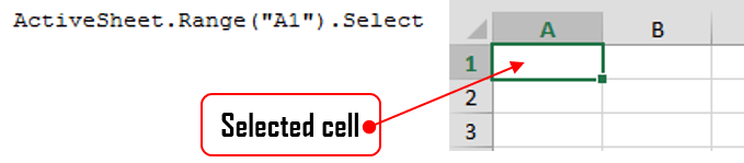
Range("A1:B2").Select 'Select the Cells A1:B2 in your Excel Worksheet
Range("A1:B2").Activate 'Activate the cells and show them on your screen (will switch to Worksheet and/or scroll to this range.
Select a cell or Range of cells using the Select method. It will be visibly marked in Excel:
Working with Range variables
The Range is a separate object variable and can be declared as other variables. As the VBA Range is an object you need to use the Set statement:
Dim myRange as Range
'...
Set myRange = Range("A1") 'Need to use Set to define myRange
The Range object defaults to your ActiveWorksheet. So beware as depending on your ActiveWorksheet the Range object will return values local to your worksheet:
Range("A1").Select
'...is the same as...
ActiveSheet.Range("A1").Select
You might want to define the Worksheet reference by Range if you want your reference values from a specifc Worksheet:
Sheets("Sheet1").Range("A1").Select 'Will always select items from Worksheet named Sheet1
The ActiveWorkbook is not same to ThisWorkbook. Same goes for the ActiveSheet. This may reference a Worksheet from within a Workbook external to the Workbook in which the macro is executed as Active references simply the currently top-most worksheet. Read more here
Range properties
The Range object contains a variety of properties with the main one being it’s Value and an the second one being its Formula.
A Range Value is the evaluated property of a cell or a range of cells. For example a cell with the formula =10+20 has an evaluated value of 20.
A Range Formula is the formula provided in the cell or range of cells. For example a cell with a formula of =10+20 will have the same Formula property.
'Let us assume A1 contains the formula "=10+20"

Debug.Print Range("A1").Value 'Returns: 30

Debug.Print Range("A1").Formula 'Returns: =10+20
Other Range properties include:
Work in progress
Worksheet Cells
A Worksheet Cells property is similar to the Range property but allows you to obtain only a SINGLE CELL, based on its row and column index. Numbering starts at 1:

The Cells property is in fact a Range object not a separate data type.
Excel facilitates a Cells function that allows you to obtain a cell from within the ActiveSheet, current top-most worksheet.
Cells(2,2).Select 'Selects B2
'...is the same as...
ActiveSheet.Cells(2,2).Select 'Select B2
Cells are Ranges which means they are not a separate data type:
Dim myRange as Range
Set myRange = Cells(1,1) 'Cell A1
Range Rows and Columns
As we all know an Excel Worksheet is divided into Rows and Columns. The Excel VBA Range object allows you to select single or multiple rows as well as single or multiple columns. There are a couple of ways to obtain Worksheet rows in VBA:
Getting an entire row or column
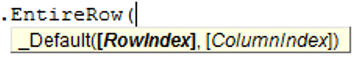
 To get and entire row of a specified Range you need to use the EntireRow property. Although, the function’s parameters suggest taking both a RowIndex and ColumnIndex it is enough just to provide the row number. Row indexing starts at 1.
 To get and entire column of a specified Range you need to use the EntireColumn property. Although, the function’s parameters suggest taking both a RowIndex and ColumnIndex it is enough just to provide the column number. Column indexing starts at 1.
Range("B2").EntireRows(1).Hidden = True 'Gets and hides the entire row 2

Range("B2").EntireColumns(1).Hidden = True 'Gets and hides the entire column 2
The three properties EntireRow/EntireColumn, Rows/Columns and Row/Column are often misunderstood so read through to understand the differences.
Get a row/column of a specified range
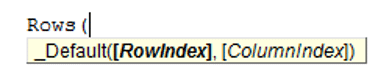 If you want to get a certain row within a Range simply use the Rows property of the Worksheet. Although, the function’s parameters suggest taking both a RowIndex and ColumnIndex it is enough just to provide the row number. Row indexing starts at 1.
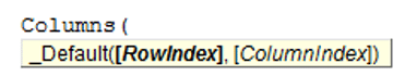 Similarly you can use the Columns function to obtain any single column within a Range. Although, the function’s parameters suggest taking both a RowIndex and ColumnIndex actually the first argument you provide will be the column index. Column indexing starts at 1.
Rows(1).Hidden = True 'Hides the first row in the ActiveSheet
'same as
ActiveSheet.Rows(1).Hidden = True

Columns(1).Hidden = True 'Hides the first column in the ActiveSheet
'same as
ActiveSheet.Columns(1).Hidden = True
To get a range of rows/columns you need to use the Range function like so:
Range(Rows(1), Rows(3)).Hidden = True 'Hides rows 1:3
'same as
Range("1:3").Hidden = True
'same as
ActiveSheet.Range("1:3").Hidden = True

Range(Columns(1), Columns(3)).Hidden = True 'Hides columns A:C
'same as
Range("A:C").Hidden = True
'same as
ActiveSheet.Range("A:C").Hidden = True
Get row/column of specified range
The above approach assumed you want to obtain only rows/columns from the ActiveSheet – the visible and top-most Worksheet. Usually however, you will want to obtain rows or columns of an existing Range. Similarly as with the Worksheet Range property, any Range facilitates the Rows and Columns property.
Dim myRange as Range
Set myRange = Range("A1:C3")

myRange.Rows.Hidden = True 'Hides rows 1:3
myRange.Columns.Hidden = True 'Hides columns A:C

Set myRange = Range("C10:F20")
myRange.Rows(2).Hidden = True 'Hides rows 11
myRange.Columns(3).Hidden = True 'Hides columns E
Getting a Ranges first row/column number
Aside from the Rows and Columns properties Ranges also facilitate a Row and Column property which provide you with the number of the Ranges first row and column.
Set myRange = Range("C10:F20")

'Get first row number
Debug.Print myRange.Row 'Result: 10
'Get first column number
Debug.Print myRange.Column 'Result: 3
Converting Column number to Excel Column
This is an often question that turns up – how to convert a column number to a string e.g. 100 to “CV”.
Function GetExcelColumn(columnNumber As Long)
    Dim div As Long, colName As String, modulo As Long
    div = columnNumber: colName = vbNullString

    Do While div > 0
        modulo = (div - 1) Mod 26
        colName = Chr(65 + modulo) & colName
        div = ((div - modulo) / 26)
    Loop

    GetExcelColumn = colName
End Function
Range Cut/Copy/Paste
Cutting and pasting rows is generally a bad practice which I heavily discourage as this is a practice that is moments can be heavily cpu-intensive and often is unaccounted for.
Copy function
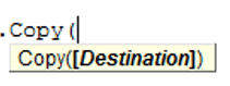 The Copy function works on a single cell, subset of cell or subset of rows/columns.
'Copy values and formatting from cell A1 to cell D1
Range("A1").Copy Range("D1")

'Copy 3x3 A1:C3 matrix to D1:F3 matrix - dimension must be same
Range("A1:C3").Copy Range("D1:F3")

'Copy rows 1:3 to rows 4:6
Range("A1:A3").EntireRow.Copy Range("A4")

'Copy columns A:C to columns D:F
Range("A1:C1").EntireColumn.Copy Range("D1")
The Copy function can also be executed without an argument. It then copies the Range to the Windows Clipboard for later Pasting.
Cut function
![]() The Cut function, similarly as the Copy function, cuts single cells, ranges of cells or rows/columns.
The Cut function, similarly as the Copy function, cuts single cells, ranges of cells or rows/columns.
'Cut A1 cell and paste it to D1
Range("A1").Cut Range("D1")

'Cut 3x3 A1:C3 matrix and paste it in D1:F3 matrix - dimension must be same
Range("A1:C3").Cut Range("D1:F3")

'Cut rows 1:3 and paste to rows 4:6
Range("A1:A3").EntireRow.Cut Range("A4")

'Cut columns A:C and paste to columns D:F
Range("A1:C1").EntireColumn.Cut Range("D1")
The Cut function can be executed without arguments. It will then cut the contents of the Range and copy it to the Windows Clipboard for pasting.
Cutting cells/rows/columns does not shift any remaining cells/rows/columns but simply leaves the cut out cells empty
PasteSpecial function
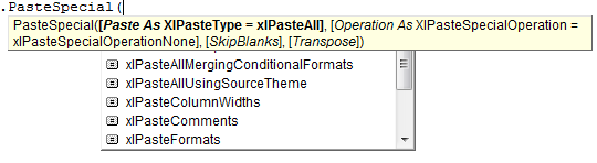 The Range PasteSpecial function works only when preceded with either the Copy or Cut Range functions. It pastes the Range (or other data) within the Clipboard to the Range on which it was executed.
Syntax
The PasteSpecial function has the following syntax:
PasteSpecial( Paste, Operation, SkipBlanks, Transpose)
The PasteSpecial function can only be used in tandem with the Copy function (not Cut)
Parameters
Paste
The part of the Range which is to be pasted. This parameter can have the following values:
| Parameter | Constant | Description | |
|---|---|---|---|
| xlPasteSpecialOperationAdd | 2 | Copied data will be added with the value in the destination cell. | |
| xlPasteSpecialOperationDivide | 5 | Copied data will be divided with the value in the destination cell. | |
| xlPasteSpecialOperationMultiply | 4 | Copied data will be multiplied with the value in the destination cell. | |
| xlPasteSpecialOperationNone | -4142 | No calculation will be done in the paste operation. | |
| xlPasteSpecialOperationSubtract | 3 | Copied data will be subtracted with the value in the destination cell. |
Operation
The paste operation e.g. paste all, only formatting, only values, etc. This can have one of the following values:
| Name | Constant | Description |
|---|---|---|
| xlPasteAll | -4104 | Everything will be pasted. |
| xlPasteAllExceptBorders | 7 | Everything except borders will be pasted. |
| xlPasteAllMergingConditionalFormats | 14 | Everything will be pasted and conditional formats will be merged. |
| xlPasteAllUsingSourceTheme | 13 | Everything will be pasted using the source theme. |
| xlPasteColumnWidths | 8 | Copied column width is pasted. |
| xlPasteComments | -4144 | Comments are pasted. |
| xlPasteFormats | -4122 | Copied source format is pasted. |
| xlPasteFormulas | -4123 | Formulas are pasted. |
| xlPasteFormulasAndNumberFormats | 11 | Formulas and Number formats are pasted. |
| xlPasteValidation | 6 | Validations are pasted. |
| xlPasteValues | -4163 | Values are pasted. |
| xlPasteValuesAndNumberFormats | 12 | Values and Number formats are pasted. |
SkipBlanks
If True then blanks will not be pasted.
Transpose
Transpose the Range before paste (swap rows with columns).
PasteSpecial Examples
'Cut A1 cell and paste its values to D1
Range("A1").Copy
Range("D1").PasteSpecial

'Copy 3x3 A1:C3 matrix and add all the values to E1:G3 matrix (dimension must be same)
Range("A1:C3").Copy
Range("E1:G3").PasteSpecial xlPasteValues, xlPasteSpecialOperationAdd
Below an example where the Excel Range A1:C3 values are copied an added to the E1:G3 Range. You can also multiply, divide and run other similar operations.
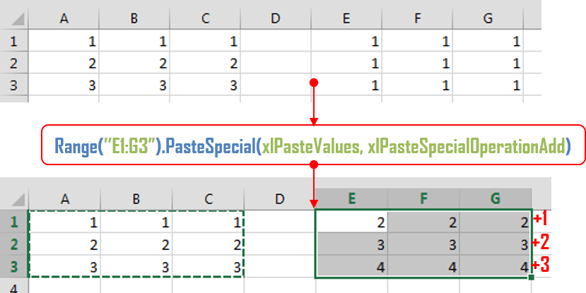
Paste
The Paste function allows you to paste data in the Clipboard to the actively selected Range. Cutting and Pasting can only be accomplished with the Paste function.
'Cut A1 cell and paste its values to D1
Range("A1").Cut
Range("D1").Select
ActiveSheet.Paste

'Cut 3x3 A1:C3 matrix and paste it in D1:F3 matrix - dimension must be same
Range("A1:C3").Cut
Range("D1:F3").Select
ActiveSheet.Paste

'Cut rows 1:3 and paste to rows 4:6
Range("A1:A3").EntireRow.Cut
Range("A4").Select
ActiveSheet.Paste

'Cut columns A:C and paste to columns D:F
Range("A1:C1").EntireColumn.Cut
Range("D1").Select
ActiveSheet.Paste
Range Clear/Delete
The Clear function
The Clear function clears the entire content and formatting from an Excel Range. It does not, however, shift (delete) the cleared cells.
Range("A1:C3").Clear
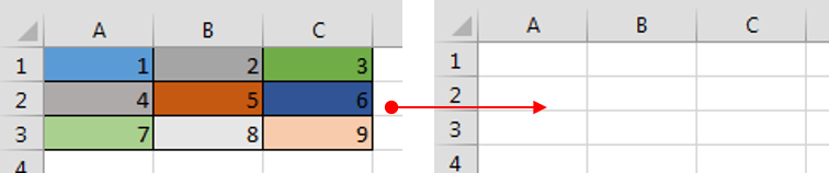
The Delete function
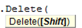 The Delete function deletes a Range of cells, removing them entirely from the Worksheet, and shifts the remaining Cells in a selected shift direction.
Although the manual Delete cell function provides 4 ways of shifting cells. The VBA Delete Shift values can only be either be xlShiftToLeft or xlShiftUp.
'If Shift omitted, Excel decides - shift up in this case
Range("B2").Delete

'Delete and Shift remaining cells left
Range("B2").Delete xlShiftToLeft

'Delete and Shift remaining cells up
Range("B2").Delete xlShiftTop

'Delete entire row 2 and shift up
Range("B2").EntireRow.Delete

'Delete entire column B and shift left
Range("B2").EntireRow.Delete
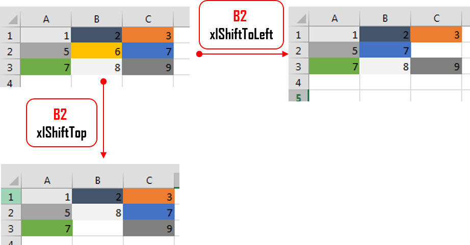
Traversing Ranges
Traversing cells is really useful when you want to run an operation on each cell within an Excel Range. Fortunately this is easily achieved in VBA using the For Each or For loops.
Dim cellRange As Range

For Each cellRange In Range("A1:C3")
  Debug.Print cellRange.Value
Next cellRange
Although this may not be obvious, beware of iterating/traversing the Excel Range using a simple For loop. For loops are not efficient on Ranges. Use a For Each loop as shown above. This is because Ranges resemble more Collections than Arrays. Read more on For vs For Each loops here
Traversing the UsedRange
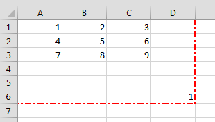 Every Worksheet has a UsedRange. This represents that smallest rectangle Range that contains all cells that have or had at some point values. In other words if the further out in the bottom, right-corner of the Worksheet there is a certain cell (e.g. E8) then the UsedRange will be as large as to include that cell starting at cell A1 (e.g. A1:E8). In Excel you can check the current UsedRange hitting CTRL+END. In VBA you get the UsedRange like this:
ActiveSheet.UsedRange
'same as
UsedRange
You can traverse through the UsedRange like this:
Dim cellRange As Range

For Each cellRange In UsedRange
  Debug.Print "Row: " & cellRange.Row & ", Column: " & cellRange.Column
Next cellRange
The UsedRange is a useful construct responsible often for bloated Excel Workbooks. Often delete unused Rows and Columns that are considered to be within the UsedRange can result in significantly reducing your file size. Read also more on the XSLB file format here
Range Addresses
The Excel Range Address property provides a string value representing the Address of the Range.
![]()
Syntax
Below the syntax of the Excel Range Address property:
Address( [RowAbsolute], [ColumnAbsolute], [ReferenceStyle], [External], [RelativeTo] )
Parameters
RowAbsolute
Optional. If True returns the row part of the reference address as an absolute reference. By default this is True.
$D$10:$G$100 'RowAbsolute is set to True
$D10:$G100 'RowAbsolute is set to False
ColumnAbsolute
Optional. If True returns the column part of the reference as an absolute reference. By default this is True.
$D$10:$G$100 'ColumnAbsolute is set to True
D$10:G$100 'ColumnAbsolute is set to False
ReferenceStyle
Optional. The reference style. The default value is xlA1. Possible values:
| Constant | Value | Description |
|---|---|---|
| xlA1 | 1 | Default. Use xlA1 to return an A1-style reference |
| xlR1C1 | -4150 | Use xlR1C1 to return an R1C1-style reference |
External
Optional. If True then property will return an external reference address, otherwise a local reference address will be returned. By default this is False.
$A$1 'Local
[Book1.xlsb]Sheet1!$A$1 'External
RelativeTo
Provided RowAbsolute and ColumnAbsolute are set to False, and the ReferenceStyle is set to xlR1C1, then you must include a starting point for the relative reference. This must be a Range variable to be set as the reference point.
Merged Ranges
![]() Merged cells are Ranges that consist of 2 or more adjacent cells. To Merge a collection of adjacent cells run Merge function on that Range.
Merged cells are Ranges that consist of 2 or more adjacent cells. To Merge a collection of adjacent cells run Merge function on that Range.
The Merge has only a single parameter – Across, a boolean which if True will merge cells in each row of the specified range as separate merged cells. Otherwise the whole Range will be merged. The default value is False.
Merge examples
To merge the entire Range:
'This will turn of any alerts warning that values may be lost
Application.DisplayAlerts = False

Range("B2:C3").Merge
This will result in the following:
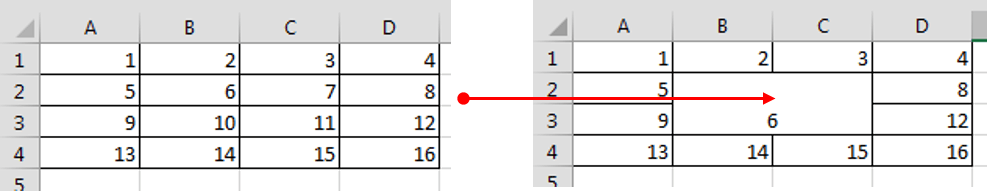
To merge just the rows set Across to True.
'This will turn of any alerts warning that values may be lost
Application.DisplayAlerts = False

Range("B2:C3").Merge True
This will result in the following:
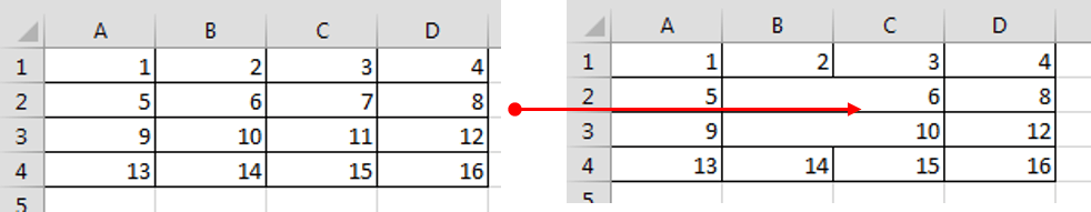
Remember that merged Ranges can only have a single value and formula. Hence, if you merge a group of cells with more than a single value/formula only the first value/formula will be set as the value/formula for your new merged Range
Checking if Range is merged
To check if a certain Range is merged simply use the Excel Range MergeCells property:
Range("B2:C3").Merge

Debug.Print Range("B2").MergeCells 'Result: True
The MergeArea
The MergeArea is a property of an Excel Range that represent the whole merge Range associated with the current Range. Say that $B$2:$C$3 is a merged Range – each cell within that Range (e.g. B2, C3..) will have the exact same MergedArea. See example below:
Range("B2:C3").Merge
Debug.Print Range("B2").MergeArea.Address 'Result: $B$2:$C$3
Named Ranges
Named Ranges are Ranges associated with a certain Name (string). In Excel you can find all your Named Ranges by going to Formulas->Name Manager. They are very useful when working on certain values that are used frequently through out your Workbook. Imagine that you are writing a Financial Analysis and want to use a common Discount Rate across all formulas. Just the address of the cell e.g. “A2”, won’t be self-explanatory. Why not use e.g. “DiscountRate” instead? Well you can do just that.
Creating a Named Range
Named Ranges can be created either within the scope of a Workbook or Worksheet:
Dim r as Range
'Within Workbook
Set r = ActiveWorkbook.Names.Add("NewName", Range("A1"))
'Within Worksheet
Set r = ActiveSheet.Names.Add("NewName", Range("A1"))
This gives you flexibility to use similar names across multiple Worksheets or use a single global name across the entire Workbook.
Listing all Named Ranges
You can list all Named Ranges using the Name Excel data type. Names are objects that represent a single NamedRange. See an example below of listing our two newly created NamedRanges:
Call ActiveWorkbook.Names.Add("NewName", Range("A1"))
Call ActiveSheet.Names.Add("NewName", Range("A1"))

Dim n As Name
For Each n In ActiveWorkbook.Names
  Debug.Print "Name: " & n.Name & ", Address: " & _
       n.RefersToRange.Address & ", Value: "; n.RefersToRange.Value
Next n

'Result:
'Name: Sheet1!NewName, Address: $A$1, Value:  1
'Name: NewName, Address: $A$1, Value:  1
SpecialCells
SpecialCells are a very useful Excel Range property, that allows you to select a subset of cells/Ranges within a certain Range.
Syntax
The SpecialCells property has the following syntax:
SpecialCells( Type, [Value] )
Parameters
Type
The type of cells to be returned. Possible values:
| Constant | Value | Description |
|---|---|---|
| xlCellTypeAllFormatConditions | -4172 | Cells of any format |
| xlCellTypeAllValidation | -4174 | Cells having validation criteria |
| xlCellTypeBlanks | 4 | Empty cells |
| xlCellTypeComments | -4144 | Cells containing notes |
| xlCellTypeConstants | 2 | Cells containing constants |
| xlCellTypeFormulas | -4123 | Cells containing formulas |
| xlCellTypeLastCell | 11 | The last cell in the used range |
| xlCellTypeSameFormatConditions | -4173 | Cells having the same format |
| xlCellTypeSameValidation | -4175 | Cells having the same validation criteria |
| xlCellTypeVisible | 12 | All visible cells |
Value
If Type is equal to xlCellTypeConstants or xlCellTypeFormulas this determines the types of cells to return e.g. with errors.
| Constant | Value |
|---|---|
| xlErrors | 16 |
| xlLogical | 4 |
| xlNumbers | 1 |
| xlTextValues | 2 |
SpecialCells examples
Get Excel Range with Constants
This will return only cells with constant cells within the Range C1:C3:
For Each r In Range("A1:C3").SpecialCells(xlCellTypeConstants)
  Debug.Print r.Value
Next r
Search for Excel Range with Errors
For Each r In ActiveSheet.UsedRange.SpecialCells(xlCellTypeFormulas, xlErrors)
  Debug.Print r.Address
Next r