Range of column in excel vba - Word и Excel - помощь в работе с программами

Excel VBA Columns Property

VBA Columns property is used to refer to columns in the worksheet. Using this property we can use any column in the specified worksheet and work with it.

When we want to refer to the cell, we use either the Range object or Cells property. Similarly, how do you refer to columns in VBA? We can refer to columns by using the “Columns” property. Look at the syntax of COLUMNS property.

Excel VBA Columns Property
- Examples
  - Example #1
  - Example #2 – Select Column Based on Variable Value
  - Example #3 – Select Column Based on Cell Value
  - Example #4 – Combination of Range & Column Property
  - Example #5 – Select Multiple Columns with Range Object
- Recommended Articles

We need to mention the column number or header alphabet to reference the column.

For example, if we want to refer to the second column, we can write the code in three ways.

Columns (2)

Columns(“B:B”)

Range (“B:B”)

Examples

You can download this VBA Columns Excel Template here – VBA Columns Excel Template

Example #1

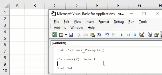
If you want to select the second column in the worksheet, then first, we need to mention the column number we need to select.

Code:

Sub Columns_Example()

  Columns (2)

End Sub

Now, put a dot (.) to choose the “Select” method.

One of the problems with this property is we do not get to see the IntelliSense list of VBA.

Code:

Sub Columns_Example()

  Columns(2).Select

End Sub

So, the above VBA codeVBA code refers to a set of instructions written by the user in the Visual Basic Applications programming language on a Visual Basic Editor (VBE) to perform a specific task.read more will select the second column of the worksheet.

Instead of mentioning the column number, we can use the column header alphabet “B” to select the second column.

Code:

Sub Columns_Example()

  Columns("B").Select
  Columns("B:B").Select

End Sub

The above codes will select column B, i.e., the second column.

Example #2 – Select Column Based on Variable Value

We can also use the variable to select the column number. For example, look at the below code now.

Code:

Sub Columns_Example()

  Dim ColNum As Integer
  ColNum = 4
  Columns(ColNum).Select

End Sub

In the above, we have declared the variable as “Integer” and assigned the value of 4 to this variable.

We have supplied this variable instead of the column number for the Column’s property. Since the variable holds the value of 4, it will select the 4th column.

Example #3 – Select Column Based on Cell Value

We have seen how to select the column based on variable value now. Next, we will see how we can select the column based on the cell value number. For example, in cell A1 we have entered the number 3.

The code below will select the column based on the number in cell A1.

Code:

Sub Columns_Example()

  Dim ColNum As Integer
  ColNum = Range("A1").Value
  Columns(ColNum).Select

End Sub

The above code is the same as the previous one. Still, the only thing we have changed here is instead of assigning the direct number to the variable. Instead, we gave a variable value as “whatever the number is in cell A1.”

Since we have a value of 3 in cell A1, it will select the third column.

Example #4 – Combination of Range & Column Property

We can also use the Columns property with the Range object. Using the Range object, we can specify the specific range. For example, look at the below code.

Code:

Sub Columns_Example1()

  Range("C1:D5").Columns(2).Select

End Sub

In the above example, we have specified the range of cells as C1 to D5. Then, using the columns property, we have specified the column number as 2 to select.

Now, in general, our second column is B. So the code has to select the “B” column but see what happens when we run the code.

It has selected the cells from D1 to D5.

In our perception, it should have selected the second column, i.e., column B. But now, it has selected the cells from D1 to D5.

It has selected these cells because before using the COLUMNS property, we have specified the range using the RANGE object as C1 to D5. Now, the property thinks within this range as the columns and selects the second column in the range C1 to D5. Therefore, D is the second column, and specified cells are D1 to D5.

Example #5 – Select Multiple Columns with Range Object

Using the Range object and Columns property, we can select multiple columns. For example, look at the below code.

Code:

Sub Columns_Example1()

  Range(Columns(2), Columns(5)).Select

End Sub

The code will select the column from the second column to the fifth column, i.e., from column B to E.

We can also write the code in this way.

Code:

Sub Columns_Example1()

  Range(Columns(B), Columns(E)).Select

End Sub

The above is the same as the previous one and selects the columns from B to E.

Like this, we can use the COLUMNS property to work with the worksheet.

A Quick Guide to Ranges and Cells

Function	Takes	Returns	Example	Gives
Range	cell address	multiple cells	.Range(«A1:A4»)	$A$1:$A$4
Cells	row, column	one cell	.Cells(1,5)	$E$1
Offset	row, column	multiple cells	Range(«A1:A2») .Offset(1,2)	$C$2:$C$3
Rows	row(s)	one or more rows	.Rows(4) .Rows(«2:4»)	$4:$4 $2:$4
Columns	column(s)	one or more columns	.Columns(4) .Columns(«B:D»)	$D:$D $B:$D

Download the Code

The Webinar

If you are a member of the VBA Vault, then click on the image below to access the webinar and the associated source code.

(Note: Website members have access to the full webinar archive.)

Introduction

This is the third post dealing with the three main elements of VBA. These three elements are the Workbooks, Worksheets and Ranges/Cells. Cells are by far the most important part of Excel. Almost everything you do in Excel starts and ends with Cells.

Generally speaking, you do three main things with Cells

Read from a cell.
Write to a cell.
Change the format of a cell.

Excel has a number of methods for accessing cells such as Range, Cells and Offset.These can cause confusion as they do similar things and can lead to confusion

In this post I will tackle each one, explain why you need it and when you should use it.

Let’s start with the simplest method of accessing cells – using the Range property of the worksheet.

Important Notes

I have recently updated this article so that is uses Value2.

You may be wondering what is the difference between Value, Value2 and the default:

' Value2
Range("A1").Value2 = 56

' Value
Range("A1").Value = 56

' Default uses value
Range("A1") = 56

Using Value may truncate number if the cell is formatted as currency. If you don’t use any property then the default is Value.

It is better to use Value2 as it will always return the actual cell value(see this article from Charle Williams.)

The Range Property

The worksheet has a Range property which you can use to access cells in VBA. The Range property takes the same argument that most Excel Worksheet functions take e.g. “A1”, “A3:C6” etc.

The following example shows you how to place a value in a cell using the Range property.

' https://excelmacromastery.com/
Public Sub WriteToCell()

    ' Write number to cell A1 in sheet1 of this workbook
    ThisWorkbook.Worksheets("Sheet1").Range("A1").Value2 = 67

    ' Write text to cell A2 in sheet1 of this workbook
    ThisWorkbook.Worksheets("Sheet1").Range("A2").Value2 = "John Smith"

    ' Write date to cell A3 in sheet1 of this workbook
    ThisWorkbook.Worksheets("Sheet1").Range("A3").Value2 = #11/21/2017#

End Sub

As you can see Range is a member of the worksheet which in turn is a member of the Workbook. This follows the same hierarchy as in Excel so should be easy to understand. To do something with Range you must first specify the workbook and worksheet it belongs to.

For the rest of this post I will use the code name to reference the worksheet.

The following code shows the above example using the code name of the worksheet i.e. Sheet1 instead of ThisWorkbook.Worksheets(“Sheet1”).

' https://excelmacromastery.com/
Public Sub UsingCodeName()

    ' Write number to cell A1 in sheet1 of this workbook
    Sheet1.Range("A1").Value2 = 67

    ' Write text to cell A2 in sheet1 of this workbook
    Sheet1.Range("A2").Value2 = "John Smith"

    ' Write date to cell A3 in sheet1 of this workbook
    Sheet1.Range("A3").Value2 = #11/21/2017#

End Sub

You can also write to multiple cells using the Range property

' https://excelmacromastery.com/
Public Sub WriteToMulti()

    ' Write number to a range of cells
    Sheet1.Range("A1:A10").Value2 = 67

    ' Write text to multiple ranges of cells
    Sheet1.Range("B2:B5,B7:B9").Value2 = "John Smith"

End Sub

You can download working examples of all the code from this post from the top of this article.

The Cells Property of the Worksheet

The worksheet object has another property called Cells which is very similar to range. There are two differences

Cells returns a range of one cell only.
Cells takes row and column as arguments.

The example below shows you how to write values to cells using both the Range and Cells property

' https://excelmacromastery.com/
Public Sub UsingCells()

    ' Write to A1
    Sheet1.Range("A1").Value2 = 10
    Sheet1.Cells(1, 1).Value2  = 10

    ' Write to A10
    Sheet1.Range("A10").Value2 = 10
    Sheet1.Cells(10, 1).Value2  = 10

    ' Write to E1
    Sheet1.Range("E1").Value2 = 10
    Sheet1.Cells(1, 5).Value2  = 10

End Sub

You may be wondering when you should use Cells and when you should use Range. Using Range is useful for accessing the same cells each time the Macro runs.

For example, if you were using a Macro to calculate a total and write it to cell A10 every time then Range would be suitable for this task.

Using the Cells property is useful if you are accessing a cell based on a number that may vary. It is easier to explain this with an example.

In the following code, we ask the user to specify the column number. Using Cells gives us the flexibility to use a variable number for the column.

' https://excelmacromastery.com/
Public Sub WriteToColumn()

    Dim UserCol As Integer
    
    ' Get the column number from the user
    UserCol = Application.InputBox(" Please enter the column...", Type:=1)
    
    ' Write text to user selected column
    Sheet1.Cells(1, UserCol).Value2 = "John Smith"

End Sub

In the above example, we are using a number for the column rather than a letter.

To use Range here would require us to convert these values to the letter/number cell reference e.g. “C1”. Using the Cells property allows us to provide a row and a column number to access a cell.

Sometimes you may want to return more than one cell using row and column numbers. The next section shows you how to do this.

Using Cells and Range together

As you have seen you can only access one cell using the Cells property. If you want to return a range of cells then you can use Cells with Ranges as follows

' https://excelmacromastery.com/
Public Sub UsingCellsWithRange()

    With Sheet1
        ' Write 5 to Range A1:A10 using Cells property
        .Range(.Cells(1, 1), .Cells(10, 1)).Value2 = 5

        ' Format Range B1:Z1 to be bold
        .Range(.Cells(1, 2), .Cells(1, 26)).Font.Bold = True

    End With

End Sub

As you can see, you provide the start and end cell of the Range. Sometimes it can be tricky to see which range you are dealing with when the value are all numbers. Range has a property called Address which displays the letter/ number cell reference of any range. This can come in very handy when you are debugging or writing code for the first time.

In the following example we print out the address of the ranges we are using:

' https://excelmacromastery.com/
Public Sub ShowRangeAddress()

    ' Note: Using underscore allows you to split up lines of code
    With Sheet1

        ' Write 5 to Range A1:A10 using Cells property
        .Range(.Cells(1, 1), .Cells(10, 1)).Value2 = 5
        Debug.Print "First address is : " _
            + .Range(.Cells(1, 1), .Cells(10, 1)).Address

        ' Format Range B1:Z1 to be bold
        .Range(.Cells(1, 2), .Cells(1, 26)).Font.Bold = True
        Debug.Print "Second address is : " _
            + .Range(.Cells(1, 2), .Cells(1, 26)).Address

    End With

End Sub

In the example I used Debug.Print to print to the Immediate Window. To view this window select View->Immediate Window(or Ctrl G)

You can download all the code for this post from the top of this article.

The Offset Property of Range

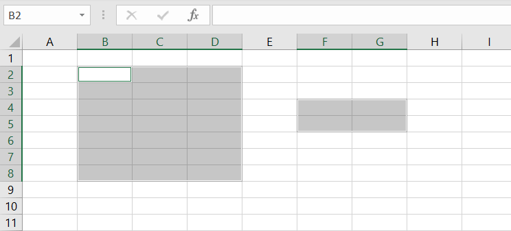
Range has a property called Offset. The term Offset refers to a count from the original position. It is used a lot in certain areas of programming. With the Offset property you can get a Range of cells the same size and a certain distance from the current range. The reason this is useful is that sometimes you may want to select a Range based on a certain condition. For example in the screenshot below there is a column for each day of the week. Given the day number(i.e. Monday=1, Tuesday=2 etc.) we need to write the value to the correct column.

We will first attempt to do this without using Offset.

' https://excelmacromastery.com/
' This sub tests with different values
Public Sub TestSelect()

    ' Monday
    SetValueSelect 1, 111.21
    ' Wednesday
    SetValueSelect 3, 456.99
    ' Friday
    SetValueSelect 5, 432.25
    ' Sunday
    SetValueSelect 7, 710.17

End Sub

' Writes the value to a column based on the day
Public Sub SetValueSelect(lDay As Long, lValue As Currency)

    Select Case lDay
        Case 1: Sheet1.Range("H3").Value2 = lValue
        Case 2: Sheet1.Range("I3").Value2 = lValue
        Case 3: Sheet1.Range("J3").Value2 = lValue
        Case 4: Sheet1.Range("K3").Value2 = lValue
        Case 5: Sheet1.Range("L3").Value2 = lValue
        Case 6: Sheet1.Range("M3").Value2 = lValue
        Case 7: Sheet1.Range("N3").Value2 = lValue
    End Select

End Sub

As you can see in the example, we need to add a line for each possible option. This is not an ideal situation. Using the Offset Property provides a much cleaner solution

' https://excelmacromastery.com/
' This sub tests with different values
Public Sub TestOffset()

    DayOffSet 1, 111.01
    DayOffSet 3, 456.99
    DayOffSet 5, 432.25
    DayOffSet 7, 710.17

End Sub

Public Sub DayOffSet(lDay As Long, lValue As Currency)

    ' We use the day value with offset specify the correct column
    Sheet1.Range("G3").Offset(, lDay).Value2 = lValue

End Sub

As you can see this solution is much better. If the number of days in increased then we do not need to add any more code. For Offset to be useful there needs to be some kind of relationship between the positions of the cells. If the Day columns in the above example were random then we could not use Offset. We would have to use the first solution.

One thing to keep in mind is that Offset retains the size of the range. So .Range(“A1:A3”).Offset(1,1) returns the range B2:B4. Below are some more examples of using Offset

' https://excelmacromastery.com/
Public Sub UsingOffset()

    ' Write to B2 - no offset
    Sheet1.Range("B2").Offset().Value2 = "Cell B2"

    ' Write to C2 - 1 column to the right
    Sheet1.Range("B2").Offset(, 1).Value2 = "Cell C2"

    ' Write to B3 - 1 row down
    Sheet1.Range("B2").Offset(1).Value2 = "Cell B3"

    ' Write to C3 - 1 column right and 1 row down
    Sheet1.Range("B2").Offset(1, 1).Value2 = "Cell C3"

    ' Write to A1 - 1 column left and 1 row up
    Sheet1.Range("B2").Offset(-1, -1).Value2 = "Cell A1"

    ' Write to range E3:G13 - 1 column right and 1 row down
    Sheet1.Range("D2:F12").Offset(1, 1).Value2 = "Cells E3:G13"

End Sub

Using the Range CurrentRegion

CurrentRegion returns a range of all the adjacent cells to the given range.

In the screenshot below you can see the two current regions. I have added borders to make the current regions clear.

A row or column of blank cells signifies the end of a current region.

You can manually check the CurrentRegion in Excel by selecting a range and pressing Ctrl + Shift + *.

If we take any range of cells within the border and apply CurrentRegion, we will get back the range of cells in the entire area.

For example
Range(“B3”).CurrentRegion will return the range B3:D14
Range(“D14”).CurrentRegion will return the range B3:D14
Range(“C8:C9”).CurrentRegion will return the range B3:D14
and so on

How to Use

We get the CurrentRegion as follows

' Current region will return B3:D14 from above example
Dim rg As Range
Set rg = Sheet1.Range("B3").CurrentRegion

Read Data Rows Only

Read through the range from the second row i.e.skipping the header row

' Current region will return B3:D14 from above example
Dim rg As Range
Set rg = Sheet1.Range("B3").CurrentRegion

' Start at row 2 - row after header
Dim i As Long
For i = 2 To rg.Rows.Count
    ' current row, column 1 of range
    Debug.Print rg.Cells(i, 1).Value2
Next i

Remove Header

Remove header row(i.e. first row) from the range. For example if range is A1:D4 this will return A2:D4

' Current region will return B3:D14 from above example
Dim rg As Range
Set rg = Sheet1.Range("B3").CurrentRegion

' Remove Header
Set rg = rg.Resize(rg.Rows.Count - 1).Offset(1)

' Start at row 1 as no header row
Dim i As Long
For i = 1 To rg.Rows.Count
    ' current row, column 1 of range
    Debug.Print rg.Cells(i, 1).Value2
Next i

Using Rows and Columns as Ranges

If you want to do something with an entire Row or Column you can use the Rows or Columns property of the Worksheet. They both take one parameter which is the row or column number you wish to access

' https://excelmacromastery.com/
Public Sub UseRowAndColumns()

    ' Set the font size of column B to 9
    Sheet1.Columns(2).Font.Size = 9

    ' Set the width of columns D to F
    Sheet1.Columns("D:F").ColumnWidth = 4

    ' Set the font size of row 5 to 18
    Sheet1.Rows(5).Font.Size = 18

End Sub

Using Range in place of Worksheet

You can also use Cells, Rows and Columns as part of a Range rather than part of a Worksheet. You may have a specific need to do this but otherwise I would avoid the practice. It makes the code more complex. Simple code is your friend. It reduces the possibility of errors.

The code below will set the second column of the range to bold. As the range has only two rows the entire column is considered B1:B2

' https://excelmacromastery.com/
Public Sub UseColumnsInRange()

    ' This will set B1 and B2 to be bold
    Sheet1.Range("A1:C2").Columns(2).Font.Bold = True

End Sub

You can download all the code for this post from the top of this article.

Reading Values from one Cell to another

In most of the examples so far we have written values to a cell. We do this by placing the range on the left of the equals sign and the value to place in the cell on the right. To write data from one cell to another we do the same. The destination range goes on the left and the source range goes on the right.

The following example shows you how to do this:

' https://excelmacromastery.com/
Public Sub ReadValues()

    ' Place value from B1 in A1
    Sheet1.Range("A1").Value2 = Sheet1.Range("B1").Value2

    ' Place value from B3 in sheet2 to cell A1
    Sheet1.Range("A1").Value2 = Sheet2.Range("B3").Value2

    ' Place value from B1 in cells A1 to A5
    Sheet1.Range("A1:A5").Value2 = Sheet1.Range("B1").Value2

    ' You need to use the "Value" property to read multiple cells
    Sheet1.Range("A1:A5").Value2 = Sheet1.Range("B1:B5").Value2

End Sub

As you can see from this example it is not possible to read from multiple cells. If you want to do this you can use the Copy function of Range with the Destination parameter

' https://excelmacromastery.com/
Public Sub CopyValues()

    ' Store the copy range in a variable
    Dim rgCopy As Range
    Set rgCopy = Sheet1.Range("B1:B5")

    ' Use this to copy from more than one cell
    rgCopy.Copy Destination:=Sheet1.Range("A1:A5")

    ' You can paste to multiple destinations
    rgCopy.Copy Destination:=Sheet1.Range("A1:A5,C2:C6")

End Sub

The Copy function copies everything including the format of the cells. It is the same result as manually copying and pasting a selection. You can see more about it in the Copying and Pasting Cells section.

Using the Range.Resize Method

When copying from one range to another using assignment(i.e. the equals sign), the destination range must be the same size as the source range.

Using the Resize function allows us to resize a range to a given number of rows and columns.

For example:

' https://excelmacromastery.com/
Sub ResizeExamples()
 
    ' Prints A1
    Debug.Print Sheet1.Range("A1").Address

    ' Prints A1:A2
    Debug.Print Sheet1.Range("A1").Resize(2, 1).Address

    ' Prints A1:A5
    Debug.Print Sheet1.Range("A1").Resize(5, 1).Address
    
    ' Prints A1:D1
    Debug.Print Sheet1.Range("A1").Resize(1, 4).Address
    
    ' Prints A1:C3
    Debug.Print Sheet1.Range("A1").Resize(3, 3).Address
    
End Sub

When we want to resize our destination range we can simply use the source range size.

In other words, we use the row and column count of the source range as the parameters for resizing:

' https://excelmacromastery.com/
Sub Resize()

    Dim rgSrc As Range, rgDest As Range
    
    ' Get all the data in the current region
    Set rgSrc = Sheet1.Range("A1").CurrentRegion

      ' Get the range destination
    Set rgDest = Sheet2.Range("A1")
    Set rgDest = rgDest.Resize(rgSrc.Rows.Count, rgSrc.Columns.Count)
    
    rgDest.Value2 = rgSrc.Value2

End Sub

We can do the resize in one line if we prefer:

' https://excelmacromastery.com/
Sub ResizeOneLine()

    Dim rgSrc As Range
    
    ' Get all the data in the current region
    Set rgSrc = Sheet1.Range("A1").CurrentRegion
    
    With rgSrc
        Sheet2.Range("A1").Resize(.Rows.Count, .Columns.Count).Value2 = .Value2
    End With
    
End Sub

Reading Values to variables

We looked at how to read from one cell to another. You can also read from a cell to a variable. A variable is used to store values while a Macro is running. You normally do this when you want to manipulate the data before writing it somewhere. The following is a simple example using a variable. As you can see the value of the item to the right of the equals is written to the item to the left of the equals.

' https://excelmacromastery.com/
Public Sub UseVariables()

    ' Create
    Dim number As Long

    ' Read number from cell
    number = Sheet1.Range("A1").Value2

    ' Add 1 to value
    number = number + 1

    ' Write new value to cell
    Sheet1.Range("A2").Value2 = number

End Sub

To read text to a variable you use a variable of type String:

' https://excelmacromastery.com/
Public Sub UseVariableText()

    ' Declare a variable of type string
    Dim text As String

    ' Read value from cell
    text = Sheet1.Range("A1").Value2

    ' Write value to cell
    Sheet1.Range("A2").Value2 = text

End Sub

You can write a variable to a range of cells. You just specify the range on the left and the value will be written to all cells in the range.

' https://excelmacromastery.com/
Public Sub VarToMulti()

    ' Read value from cell
    Sheet1.Range("A1:B10").Value2 = 66

End Sub

You cannot read from multiple cells to a variable. However you can read to an array which is a collection of variables. We will look at doing this in the next section.

How to Copy and Paste Cells

If you want to copy and paste a range of cells then you do not need to select them. This is a common error made by new VBA users.

Note: We normally use Range.Copy when we want to copy formats, formulas, validation. If we want to copy values it is not the most efficient method.
I have written a complete guide to copying data in Excel VBA here.

You can simply copy a range of cells like this:

Range("A1:B4").Copy Destination:=Range("C5")

Using this method copies everything – values, formats, formulas and so on. If you want to copy individual items you can use the PasteSpecial property of range.

It works like this

Range("A1:B4").Copy
Range("F3").PasteSpecial Paste:=xlPasteValues
Range("F3").PasteSpecial Paste:=xlPasteFormats
Range("F3").PasteSpecial Paste:=xlPasteFormulas

The following table shows a full list of all the paste types

Paste Type
xlPasteAll
xlPasteAllExceptBorders
xlPasteAllMergingConditionalFormats
xlPasteAllUsingSourceTheme
xlPasteColumnWidths
xlPasteComments
xlPasteFormats
xlPasteFormulas
xlPasteFormulasAndNumberFormats
xlPasteValidation
xlPasteValues
xlPasteValuesAndNumberFormats

Reading a Range of Cells to an Array

You can also copy values by assigning the value of one range to another.

Range("A3:Z3").Value2 = Range("A1:Z1").Value2

The value of range in this example is considered to be a variant array. What this means is that you can easily read from a range of cells to an array. You can also write from an array to a range of cells. If you are not familiar with arrays you can check them out in this post.

The following code shows an example of using an array with a range:

' https://excelmacromastery.com/
Public Sub ReadToArray()

    ' Create dynamic array
    Dim StudentMarks() As Variant

    ' Read 26 values into array from the first row
    StudentMarks = Range("A1:Z1").Value2

    ' Do something with array here

    ' Write the 26 values to the third row
    Range("A3:Z3").Value2 = StudentMarks

End Sub

Keep in mind that the array created by the read is a 2 dimensional array. This is because a spreadsheet stores values in two dimensions i.e. rows and columns

Going through all the cells in a Range

Sometimes you may want to go through each cell one at a time to check value.

You can do this using a For Each loop shown in the following code

' https://excelmacromastery.com/
Public Sub TraversingCells()

    ' Go through each cells in the range
    Dim rg As Range
    For Each rg In Sheet1.Range("A1:A10,A20")
        ' Print address of cells that are negative
        If rg.Value < 0 Then
            Debug.Print rg.Address + " is negative."
        End If
    Next

End Sub

You can also go through consecutive Cells using the Cells property and a standard For loop.

The standard loop is more flexible about the order you use but it is slower than a For Each loop.

' https://excelmacromastery.com/
Public Sub TraverseCells()
 
    ' Go through cells from A1 to A10
    Dim i As Long
    For i = 1 To 10
        ' Print address of cells that are negative
        If Range("A" & i).Value < 0 Then
            Debug.Print Range("A" & i).Address + " is negative."
        End If
    Next
 
    ' Go through cells in reverse i.e. from A10 to A1
    For i = 10 To 1 Step -1
        ' Print address of cells that are negative
        If Range("A" & i) < 0 Then
            Debug.Print Range("A" & i).Address + " is negative."
        End If
    Next
 
End Sub

Formatting Cells

Sometimes you will need to format the cells the in spreadsheet. This is actually very straightforward. The following example shows you various formatting you can add to any range of cells

' https://excelmacromastery.com/
Public Sub FormattingCells()

    With Sheet1

        ' Format the font
        .Range("A1").Font.Bold = True
        .Range("A1").Font.Underline = True
        .Range("A1").Font.Color = rgbNavy

        ' Set the number format to 2 decimal places
        .Range("B2").NumberFormat = "0.00"
        ' Set the number format to a date
        .Range("C2").NumberFormat = "dd/mm/yyyy"
        ' Set the number format to general
        .Range("C3").NumberFormat = "General"
        ' Set the number format to text
        .Range("C4").NumberFormat = "Text"

        ' Set the fill color of the cell
        .Range("B3").Interior.Color = rgbSandyBrown

        ' Format the borders
        .Range("B4").Borders.LineStyle = xlDash
        .Range("B4").Borders.Color = rgbBlueViolet

    End With

End Sub

Main Points

The following is a summary of the main points

Range returns a range of cells
Cells returns one cells only
You can read from one cell to another
You can read from a range of cells to another range of cells.
You can read values from cells to variables and vice versa.
You can read values from ranges to arrays and vice versa
You can use a For Each or For loop to run through every cell in a range.
The properties Rows and Columns allow you to access a range of cells of these types

What’s Next?

Free VBA Tutorial If you are new to VBA or you want to sharpen your existing VBA skills then why not try out the The Ultimate VBA Tutorial.

Related Training: Get full access to the Excel VBA training webinars and all the tutorials.

(NOTE: Planning to build or manage a VBA Application? Learn how to build 10 Excel VBA applications from scratch.)

Источник

Свойства Column и Columns объекта Range в VBA Excel. Возвращение номера первого столбца и обращение к столбцам смежных и несмежных диапазонов.

Range.Column — свойство, которое возвращает номер первого столбца в указанном диапазоне.

Свойство Column объекта Range предназначено только для чтения, тип данных — Long.

Если диапазон состоит из нескольких областей (несмежный диапазон), свойство Range.Column возвращает номер первого столбца в первой области указанного диапазона:

Range(«B2:F10»).Select

MsgBox Selection.Column ‘Результат: 2

Range(«E1:F8,D4:G13,B2:F10»).Select

MsgBox Selection.Column ‘Результат: 5

Для возвращения номеров первых столбцов отдельных областей несмежного диапазона используется свойство Areas объекта Range:

Range(«E1:F8,D4:G13,B2:F10»).Select

MsgBox Selection.Areas(1).Column ‘Результат: 5

MsgBox Selection.Areas(2).Column ‘Результат: 4

MsgBox Selection.Areas(3).Column ‘Результат: 2

Свойство Range.Columns

Range.Columns — свойство, которое возвращает объект Range, представляющий коллекцию столбцов в указанном диапазоне.

Чтобы возвратить один столбец заданного диапазона, необходимо указать его порядковый номер (индекс) в скобках:

Set myRange = Range(«B4:D6»).Columns(1) ‘Возвращается диапазон: $B$4:$B$6

Set myRange = Range(«B4:D6»).Columns(2) ‘Возвращается диапазон: $C$4:$C$6

Set myRange = Range(«B4:D6»).Columns(3) ‘Возвращается диапазон: $D$4:$D$6

Самое удивительное заключается в том, что выход индекса столбца за пределы указанного диапазона не приводит к ошибке, а возвращается диапазон, расположенный за пределами исходного диапазона (отсчет начинается с первого столбца заданного диапазона):

MsgBox Range(«B4:D6»).Columns(7).Address ‘Результат: $H$4:$H$6

Если указанный объект Range является несмежным, состоящим из нескольких смежных диапазонов (областей), свойство Columns возвращает коллекцию столбцов первой области заданного диапазона. Для обращения к столбцам других областей указанного диапазона используется свойство Areas объекта Range:

Range(«E1:F8,D4:G13,B2:F10»).Select

MsgBox Selection.Areas(1).Columns(2).Address ‘Результат: $F$1:$F$8

MsgBox Selection.Areas(2).Columns(2).Address ‘Результат: $E$4:$E$13

MsgBox Selection.Areas(3).Columns(2).Address ‘Результат: $C$2:$C$10

Определение количества столбцов в диапазоне:

Dim c As Long

c = Range(«D5:J11»).Columns.Count

MsgBox c ‘Результат: 7

Буква вместо номера

Если в качестве индекса столбца используется буква, она соответствует порядковому номеру этой буквы на рабочем листе:

"A" = 1;
"B" = 2;
"C" = 3;

и так далее.

Пример использования буквенного индекса вместо номера столбца в качестве аргумента свойства Columns объекта Range:

Range(«G2:K10»).Select

MsgBox Selection.Columns(2).Address ‘Результат: $H$2:$H$10

MsgBox Selection.Columns(«B»).Address ‘Результат: $H$2:$H$10

Обратите внимание, что свойство Range("G2:K10").Columns("B") возвращает диапазон $H$2:$H$10, а не $B$2:$B$10.

Источник

Ranges are a key concept in Excel, and knowing how to work with them is essential for anyone who wants to program or automate their work using Excel VBA.

In this tutorial, we’ll take a look at how to work with Excel ranges in VBA. We’ll start by discussing what a Range object is. Then, we’ll look at the different ways of referencing a range. Lastly, we’ll explore various examples of how to work with ranges using VBA code.

Excel VBA: The Range object

The Excel VBA Range object is used to represent a range in a worksheet. A range can be a cell, a group of cells, or even all the 17,179,869,184 cells in a sheet.

When programming with Excel VBA, the Range object is going to be your best friend. That’s because much of your work will focus on manipulating data within sheets. Understanding how to work with the Range object will make it easier for you to perform various actions on cells, such as changing their values, sorting, or doing a copy-paste.

The following is the Excel object hierarchy:

Application > Workbook > Worksheet > Range

You can see that the Excel VBA Range object is a property of the Worksheet object. This means that you can access a range by specifying the name of the sheet and the cell address you want to work with. When you don’t specify a sheet name, by default Excel will look for the range in the active sheet. For example, if Sheet1 is active, then both of these lines will refer to the same cell range:

Range("A1") 
Worksheets("Sheet1").Range("A1")

Let’s have a closer look at how to reference a range in the section below.

Referencing a range of cells in Excel VBA

Referring to a Range object in Excel VBA can be done in several ways. We’ll discuss the basic syntax and some alternatives that you might want to use, depending on your needs.

Excel VBA: Syntax for specifying a cell range

To refer to a range that consists of one cell, for example, cell D5, you can use the syntax below:

Range("D5")

To refer to a range of cells, you have two acceptable syntaxes. For example, A1 through D5 can be specified using any one below:

Range("A1:D5")
Range("A1", "D5")

To refer to a range outside the active sheet, you need to include the worksheet name. Here’s an example:

Worksheets("Sheet1").Range("A1:D5")

To refer to an entire row, for example, Row 5:

Range("5:5")

To refer to an entire column, for example, Column D:

Range("D:D")

Excel VBA also allows you to refer to multiple ranges at once by using a comma to separate each area. For example, see the below syntax used for referring to all ranges shown in the image:

Range("B2:D8, F4:G5")

Tip: Notice that all of the syntaxes above use double quotes to enclose the range address. To make it quicker for you to type, you can use shortcuts that involve using square brackets without quotes, as shown in the table below:

Syntax	Shortcut
`Range("D5")`	`[D5]`
`Range("A1:D5")`	`[A1:D5]`
`Range("5:5")`	`[5:5]`
`Range("B2:D8, F4:G5")`	`[B2:D8, F4:G5]`

Excel VBA: Referencing a named range

You have probably already used named ranges in your worksheets. They can be found under Name Manager in the Formulas tab.

To refer to a range named MyRange, use the following code:

Range("MyRange")

Remember to enclose the range’s name in double quotes. Otherwise, Excel thinks that you’re referring to a variable.

Alternatively, you can also use the shortcut syntax discussed previously. In this case, double quotes aren’t used:

[MyRange]

Excel VBA: Referencing a range using the Cells property

Another way to refer to a range is by using the Cells property. This property takes two arguments:

Cells(Row, Column)

You must use a numeric value for Row, but you may use either a numeric or string value for Column. Both of these lines refer to cell D5:

Cells(5, "D") 
Cells(5, 4)

The advantage of using the Cells property to refer to ranges becomes clear when you need to loop through rows or columns. You can create a more readable piece of code by using variables as the Cells arguments in a looping.

Excel VBA: Referencing a range using the Offset property

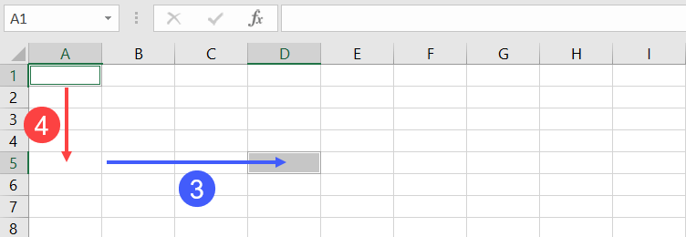
The Offset property provides another handy means for referring to ranges. It allows you to refer to a cell based on the location of another cell, such as the active cell.

Like the Cells property, the Offset property has two parameters. The first determines how many rows to offset, while the second represents the number of columns to offset. Here is the syntax:

Range.Offset(RowOffset, ColumnOffset)

For example, the following code refers to cell D5 from cell A1:

Range("A1").Offset(4,3)

The negative numbers refer to cells that are above or below the range of values. For example, a -2 row offset refers to two rows above the range, and a -1 column offset refers to a column to the left of the range. The following example refers to cell A1:

Range("D3").Offset(-2, -3)

If you need to go over only a row or a column, but not both, you don’t have to enter both the row and the column parameters. You can also use 0 as one or both of the arguments. For example, the following lines refer to D5:

Range("D5").Offset(0, 0)
Range("D2").Offset(3, 0)
Range("G5").Offset(, -3)

Let’s take a look at some of the most common range examples. These examples will show you how to use VBA to select and manipulate ranges in your worksheets. Some of these examples are complete procedures, while others are code snippets that you can just copy-paste to your own Sub to try.

Excel VBA: Select a range of cells

To select a range of cells, use the Select method.

The following line selects a range from A1 to D5 in the active worksheet:

Range("A1:D5").Select

To select a range from A1 to the active cell, use the following line:

Range("A1", ActiveCell).Select

The following code selects from the active cell to 3 rows below the active cell and five columns to the right:

Range(ActiveCell, ActiveCell.Offset(3, 5)).Select

It’s important to note that when you need to select a range on a specific worksheet, you need to ensure that the correct worksheet is active. Otherwise, an error will occur. For example, you want to select B2 to J5 on Sheet1. The following code will generate an error if Sheet1 is not active:

Worksheets("Sheet1").Range("B2:J5").Select

Instead, use these two lines of code to make your code work as expected:

Worksheets("Sheet1").Activate 
Range("B2:J5").Select

Excel VBA: Set values to a range

The following statement sets a value of 100 into cell C7 of the active worksheet:

Range("C7").Value = 100

The Value property allows you to represent the value of any cell in a worksheet. It’s a read/write property, so you can use it for both reading and changing values.

You can also set values of a range of any size. The following statement enters the text “Hello” into each cell in the range A1:C7 in Sheet2:

Worksheets("Sheet2").Range("A1:C7").Value = "Hello"

Value is the default property for a Range object. This means that if you don’t provide any properties in your range, Excel will use this Value property.

Both of the following lines enter a value of 100 into cell C7 of the active worksheet:

Range("C7").Value = 100
Range("C7") = 100

Excel VBA: Copy range to another sheet

To copy and paste a range in Excel VBA, you use the Copy and Paste methods. The Copy method copies a range, and the Paste method pastes it into a worksheet. It might look a bit complicated but let’s see what each does with an example below.

Let’s say you have Orders data, as shown in the below screenshot, which is imported from Airtable every day using Coupler.io. This tool allows users to do it automatically on the schedule they want with just a few clicks and no coding required.

In addition, they can combine data from other different sources (such as Jira, Mailchimp, etc.) into one destination for analysis purposes.

As you can see, the data starts from B2. You want to copy only range B2:C11 and paste them to Sheet2 at the same address. The following is an example Sub you can use:

Sub CopyRangeToAnotherSheet()
    Sheets("Sheet1").Activate
    Range("B2:C11").Select
    Selection.Copy
    
    Sheets("Sheet2").Activate
    Range("B2").Select
    ActiveSheet.Paste
End Sub

Alternatively, you can also use a single line of code as shown below:

Sub CopyRangeToAnotherSheet2()
    Worksheets("Sheet1").Range("B2:C11").Copy Worksheets("Sheet2").Range("B2")
End Sub

The above Sub procedure takes advantage of the fact that the Copy method can use an argument that corresponds to the destination range for the copy operation. Notice that actually, you don’t have to select a range before doing something with it.

Excel VBA: Dynamic range example

In many cases, you may need to copy a range of cells but don’t know exactly how many rows and columns it has. For example, if you use Coupler.io or other integration tools to import data from an external app into Excel on a daily schedule, the number of rows may change over time.

How can you determine this dynamic range? One solution is to use the CurrentRegion property. This property returns an Excel VBA Range object within its boundaries. As long as the data is surrounded by one empty row and one empty column, you can select it with CurrentRegion.

The following line selects the contiguous range around Cell B2:

Range("B2").CurrentRegion.Select

Now, let’s say you want to select only Columns B and C of the range, and from the second row, you can use the following line:

Range("B2", Range("C2").End(xlDown)).Select

You can now do whatever you want with your selected range — copy or move it to another sheet, format it, and so on.

If you want to find the last row of a used range using Excel VBA, it’s also possible without selecting anything. Here’s the line you can use to find the row number of Column B’s last row data:

' Find the row number of Column B's last row data
RowNumOfLastRow = Cells(Rows.Count, 2).End(xlUp).Row


' Result: 11
MsgBox RowNumOfLastRow

Excel VBA: Loop for each cell in a range

For looping each cell in a range, the For Each loop is an excellent choice. This type of loop is great for looping through a collection of objects such as cells in a range, worksheets in a workbook, or other collections.

The following procedure shows how to loop through each cell in Range B2:K11. We use an object variable named Obj, which refers to the cell being processed. Within the loop, the code checks if the cell contains a formula and then sets its color to blue.

Sub LoopForEachCell()
    Dim obj As Range
    For Each obj In Range("B2:K11")
        If obj.HasFormula Then obj.Font.Color = vbBlue
    Next obj
End Sub

Excel VBA: Loop for each row in a range

When looping through rows (or columns), you can use the Cells property to refer to a range of cells. This makes your code more readable compared to when you’re using the Range syntax.

For example, to loop for each row in range B2:K11 and bold all the cells from Column I to K, you might write a loop like this:

Sub LoopForEachRow()
    For i = 1 To 11
        Range("I" & i & ":K" & i).Font.Bold = True
    Next i
End Sub

Instead of typing in a range address, you can use the Cells property to make the loop easier to read and write. For example, the code below uses the Cells and Resize properties to find the required cell based on the active cell:

Sub LoopForEachRow2()
    For i = 1 To 11
        Cells(i, "I").Resize(, 3).Font.Bold = True
    Next i
End Sub

Excel VBA: Clear a range

There are three ways to clear a range in Excel VBA.

The first is to use the Clear method, which will clear the entire range, including cell contents and formatting.

The second is to use the ClearContents method, which will clear the contents of the range but leave the formatting intact.

The third is to use the ClearFormats method, which will clear the formatting of the range but leave the contents intact.

For example, to clear a range B1 to M15, you can use one of the following lines of code below, based on your needs:

Range("B1:M15").Clear
Range("B1:M15").ClearContents
Range("B1:M15").ClearFormats

Excel VBA: Delete a range

When deleting a range, it differs from just clearing a range. That’s because Excel shifts the remaining cells around to fill up your deleted range.

The code below deletes Row 5 using the Delete method:

Range("5:5").Delete

To delete a range that is not a complete row or column, you have to provide an argument (such as xlToLeft, xlUp — based on your needs) that indicates how Excel should shift the remaining cells.

For example, the following code deletes cell B2 to M10, then fills the resulting gap by shifting the other cells to the left:

Range("B2:M10").Delete xlToLeft

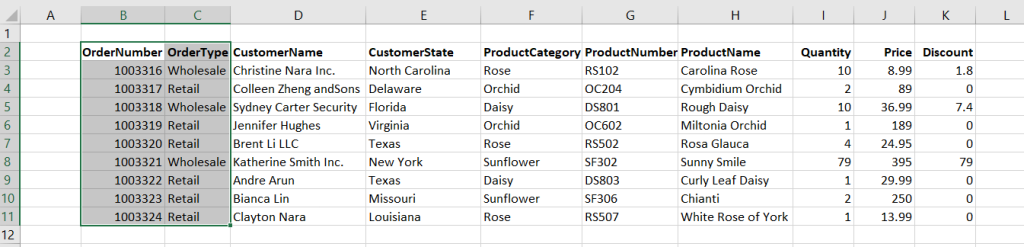
Excel VBA: Delete rows with a specific condition in a range

You can also use a VBA code to delete rows with a specific condition. For example, let’s try to delete all the rows with a discount of 0 from the below sheet:

Here’s an example Sub you may want to use:

Sub DeleteWithCondition()
    For i = 3 To 11
        If Cells(i, "F").Value = 0 Then
            Cells(i, 1).EntireRow.Delete
        End If
    Next i
End Sub

The above code loops from Row 3 to 11. In each loop, it checks the discount value in Column F and removes the entire row if the value equals 0.

Excel VBA: Find values in a range

With the below data, suppose you want to find if there is an order with OrderNumber equal to 1003320 and output its cell address.

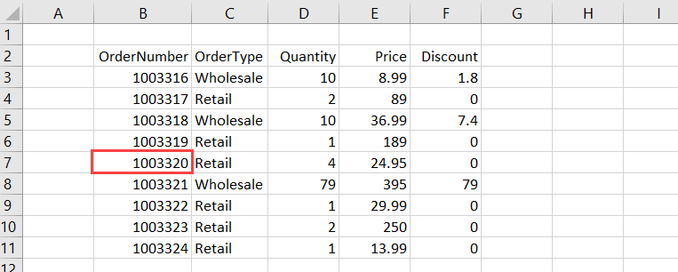
You can use the Find method in this case, as shown in the below code:

Sub FindOrder()
    Dim Rng As Range
     
    Set Rng = Range("B3:B11").Find("1003320")
     
    If Rng Is Nothing Then
        MsgBox "The OrderNumber not found."
    Else
        MsgBox Rng.Address
    End If

End Sub

The output of the above code will be the first occurrence of the search value in the specified range. If the value is not found, a message box showing info that the order is not found will appear.

Excel VBA: Add alрhаbеtѕ using Rаngе .Offset

The following is an example of a Sub that adds alphabets A-Z in a range. The code uses Offset to refer to a cell below the active cell in a loop.

Sub AddAlphabetsAZ()
    Dim i As Integer
    
    ' Use 97 To 122 for lowercase letters
    For i = 65 To 90
        ActiveCell.Value = Chr(i)
        ActiveCell.Offset(1, 0).Select
    Next i
End Sub

To use the Sub, ѕеlесt a сеll where you want tо start thе alphabets. Then, run it by pressing F5. The code will insert A-Z to the cells downward.

Excel VBA: Add auto-numbers to a range with a variable from user input

Juѕt lіkе inserting alphabets as shown in the previous example, you саn аlѕо іnѕеrt auto-numbers іn уоur worksheet automatically. This can be helpful when you work with large data.

The following is an example of a Sub that adds auto-numbers to your Excel sheet:

Sub AddAutoNumbers()
    Dim i As Integer
    
    On Error GoTo ErrorHandler
    
    i = InputBox("Enter the maximum number: ", "Enter a value")
    
    For i = 1 To i
        ActiveCell.Value = i
        ActiveCell.Offset(1, 0).Select
    Next i
    
ErrorHandler:
    Exit Sub
End Sub

Tо uѕе the соdе, уоu need tо ѕеlесt the сеll frоm where you want tо start thе auto-numbеrѕ. Then, run the Sub. In the message box that appears, enter the maximum value for the auto-numbers and сlісk OK.

Excel VBA: Sum a range

Imagine that you have written a Sub procedure to import Orders.csv into an Excel sheet:

By the way, you can automate import of CSV to Excel without any coding if you use Coupler.io

You want to sum up all the discount values and put the result in J12. The following code that utilizes the Sum worksheet function would handle that:

Sub GetTotalDiscount()
    Range("J12") = WorksheetFunction.Sum(Range("J2:J10"))
End Sub

Excel VBA: Sort a range

The Sort method sorts values in a range based on the criteria you provide.

Suppose you have the following sheet:

To sort the above data based оn thе vаluеѕ іn Column D, you can use the following code:

Sub SortBySingleColumn()
    Range("A1:E10").Sort Key1:=Range("D1"), Order1:=xlAscending, Header:=xlYes
End Sub

You can also sort the range by multiple columns. For example, to sort by Column B and Column D, here’s an example code you can use:

Sub SortByMultipleColumns()
    Range("A1:E10").Sort _
        Key1:=Range("B1"), Order1:=xlAscending, _
        Key2:=Range("D1"), Order2:=xlAscending, _
        Header:=xlYes
End Sub

Here are the arguments used in the above methods:

Kеу: It specifies the field you want to use in ѕоrting thе data.
Ordеr: It ѕресіfies whеthеr уоu wаnt tо sort the dаtа іn аѕсеndіng or dеѕсеndіng order.
Header: It spесіfies whеthеr уоur data hаѕ hеаdеrѕ оr nоt.

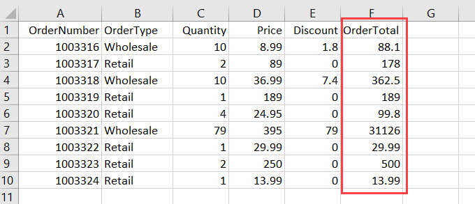
Excel VBA: Range to array

Arrays are powerful because they can actually make the code run faster. Especially when working with large data, you can use arrays to make all the processing happen in memory and then write the data to the sheet once.

For example, suppose you have the following sheet:

The following Sub uses a variable X, which is a Variant data type, to store the value of Range A2:E10. Variants can hold any type of data, including arrays.

Sub RangeToArray()
    Dim X As Variant
    X = Range("A2:E10")
End Sub

You can then treat the X variable as though it were an array. The following line returns the value of cell A6:

MsgBox X(5, 1)
' Result: 1003320

Now, let’s say you want to calculate the total order using the following calculation:

Quantity * Price - Discount

Rather than doing calculation and writing the result for each row using a looping, you can store the calculation result in an array OrderTotal as shown in the below code and write the result once:

Sub CalculateTotalOrder()
    Dim X As Variant, OrderTotal As Variant
    X = Range("A2:E10")
    
    ReDim OrderTotal(UBound(X))
    
    For i = LBound(X) To UBound(X)
        OrderTotal(i - 1) = X(i, 3) * X(i, 4) - X(i, 5)
    Next i
    
    Range("F1") = "OrderTotal"
    
    Range("F2").Resize(UBound(OrderTotal)) = _
        Application.Transpose(OrderTotal)
    
End Sub

Here’s the final result:

Subscript out of range: Excel VBA Runtime error 9

This error message often happens when you try to access a range of cells in a worksheet that has been deleted or renamed.

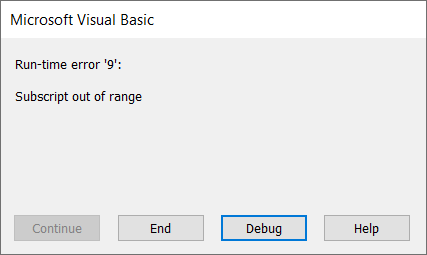
Figure 4. Excel VBA Subscript out of range error

Let’s say your code expected a worksheet named Setting. For some reason, this sheet is renamed Settings. So, the error occurs every time the below Sub runs:

Sub GetSettings()
    Worksheets("Setting").Select
    x = Range("A1").Value
End Sub

To prevent the runtime error happening again, you may want to add an error handler code like this below:

Sub GetSettings()
    On Error Resume Next

    ws = Worksheets("Setting")
    Name = ws.Name
    
    If Not Err.Number = 0 Then
        MsgBox "Expected to find a Setting worksheet, but it is missing."
        Exit Sub
    End If
    On Error GoTo 0
    
    ws.Select
    x = Range("A1").Value
End Sub

Excel VBA Range — Final words

Thank you for reading our Excel VBA Range tutorial. We hope that you’ve found it helpful! And if there’s anything else about Excel programming or other topics that interest you, be sure to check out our other Excel tutorials.

In addition, you may find that Coupler.io is a valuable tool for you if you’re looking for an easy way to pull and combine your data from multiple sources into one destination for analysis and reporting. This tool also lets you specify the range address of your imported data so you can keep all of your calculations (including. formulas) in the sheets.

Thanks again for reading, and happy coding!

Senior analyst programmer

Back to Blog

Focus on your business

goals while we take care of your data!

Try Coupler.io

Источник

Private Sub CommandButton1_Click()
Columns(«F:G»).Select
Selection.Delete
End Sub

here is some code I tested with a button on a sheet. You could just substitute the column letter with you variable. I believe you would leave out the » marks if you use a variable.

Not sure if its what you are looking for.

DaK

Thanks, I’ve tried that…

With «NCN» as my variable, this is where my code falls apart…

ActiveSheet.Columns(NCN, NCN + 10).Select (The range symbol «:» is not allowed in this set up)

Thanks again for any and all help!

Here’s one way to do it:

Range(Columns(NCN),Columns(NCN + 10)).Select

HTH,

Russell

EDIT: OOPS! Was thinking of something else when I gave this line earlier:

Columns(NCN & «:» & NCN + 10).Select

Thanks Russell.

Am I missing something though? I tried that before too, and it doesn’t work. Logically, it should (I think), but for some reason it’s not… aaarrrggghh! :rolleyes:

Columns will only take a number or the column letters in a string (such as Columns(«E:H») ).

The other way works just peachy though. :LOL:

Russell-

If «the other way» you’re talking about is:

Range(Columns(NCN),Columns(NCN + 10)).Select

I’ve tried that and it doesn’t work (btw, I know my variable is valid b/c it works in other apps).

If the above is not «the other way» you were talking about, could you please specify what is? Thanks again for your help… this problem has been haunting me for a couple weeks now…

Hi jkeys:

One of the ways to accomplish that would be to use the following code …

Code:

cells(1,NCN).resize(rows.Count,10).select

Does it help?

jkeyes said:

Russell-

If «the other way» you’re talking about is:

Range(Columns(NCN),Columns(NCN + 10)).Select

I’ve tried that and it doesn’t work (btw, I know my variable is valid b/c it works in other apps).

If the above is not «the other way» you were talking about, could you please specify what is? Thanks again for your help… this problem has been haunting me for a couple weeks now…

It works for me. What is the value of NCN when the code runs? If it is 0 or less, or if it is 247 or greater, then it won’t work. Otherwise it will. Here is the code that I used to test it.

Code:

Sub Test()
    Dim NCN As Integer
    
    NCN = 5
    Range(Columns(NCN), Columns(NCN + 10)).Select
End Sub

Hey Russ…I’m new here because of your little dittie above. I was close but the formatting can drive you nuts and you got me straightened out. Thanks a bunch. Crazy…11 years after you posted this. I love me some interwebs!

Источник

Excel VBA Columns Property

Table of contents

Examples

Example #1

Example #2 – Select Column Based on Variable Value

Example #3 – Select Column Based on Cell Value

Example #4 – Combination of Range & Column Property

Example #5 – Select Multiple Columns with Range Object

Recommended Articles

A Quick Guide to Ranges and Cells

Download the Code

The Webinar

Introduction

Important Notes

The Range Property

The Cells Property of the Worksheet

Using Cells and Range together

The Offset Property of Range

Using the Range CurrentRegion

How to Use

Read Data Rows Only

Remove Header

Using Rows and Columns as Ranges

Using Range in place of Worksheet

Reading Values from one Cell to another

Using the Range.Resize Method

Reading Values to variables

How to Copy and Paste Cells

Reading a Range of Cells to an Array

Going through all the cells in a Range

Formatting Cells

Main Points

What’s Next?

Свойство Range.Columns

Буква вместо номера

Excel VBA: The Range object

Referencing a range of cells in Excel VBA

Excel VBA: Syntax for specifying a cell range

Excel VBA: Referencing a named range

Excel VBA: Referencing a range using the Cells property

Excel VBA: Referencing a range using the Offset property

Excel VBA: Select a range of cells

Excel VBA: Set values to a range

Excel VBA: Copy range to another sheet

Excel VBA: Dynamic range example

Excel VBA: Loop for each cell in a range

Excel VBA: Loop for each row in a range

Excel VBA: Clear a range

Excel VBA: Delete a range

Excel VBA: Delete rows with a specific condition in a range

Excel VBA: Find values in a range

Excel VBA: Add alрhаbеtѕ using Rаngе .Offset

Excel VBA: Add auto-numbers to a range with a variable from user input

Excel VBA: Sum a range

Excel VBA: Sort a range

Excel VBA: Range to array

Subscript out of range: Excel VBA Runtime error 9

Excel VBA Range — Final words

Focus on your business goals while we take care of your data!

Focus on your business

goals while we take care of your data!