
Вставка формулы со ссылками в стиле A1 и R1C1 в ячейку (диапазон) из кода VBA Excel. Свойства Range.FormulaLocal и Range.FormulaR1C1Local.
Свойство Range.FormulaLocal
FormulaLocal — это свойство объекта Range, которое возвращает или задает формулу на языке пользователя, используя ссылки в стиле A1.
В качестве примера будем использовать диапазон A1:E10, заполненный числами, которые необходимо сложить построчно и результат отобразить в столбце F:

Примеры вставки формул суммирования в ячейку F1:
|
Range(«F1»).FormulaLocal = «=СУММ(A1:E1)» Range(«F1»).FormulaLocal = «=СУММ(A1;B1;C1;D1;E1)» |
Пример вставки формул суммирования со ссылками в стиле A1 в диапазон F1:F10:
|
Sub Primer1() Dim i As Byte For i = 1 To 10 Range(«F» & i).FormulaLocal = «=СУММ(A» & i & «:E» & i & «)» Next End Sub |
В этой статье я не рассматриваю свойство Range.Formula, но если вы решите его применить для вставки формулы в ячейку, используйте англоязычные функции, а в качестве разделителей аргументов — запятые (,) вместо точек с запятой (;):
|
Range(«F1»).Formula = «=SUM(A1,B1,C1,D1,E1)» |
После вставки формула автоматически преобразуется в локальную (на языке пользователя).
Свойство Range.FormulaR1C1Local
FormulaR1C1Local — это свойство объекта Range, которое возвращает или задает формулу на языке пользователя, используя ссылки в стиле R1C1.
Формулы со ссылками в стиле R1C1 можно вставлять в ячейки рабочей книги Excel, в которой по умолчанию установлены ссылки в стиле A1. Вставленные ссылки в стиле R1C1 будут автоматически преобразованы в ссылки в стиле A1.
Примеры вставки формул суммирования со ссылками в стиле R1C1 в ячейку F1 (для той же таблицы):
|
‘Абсолютные ссылки в стиле R1C1: Range(«F1»).FormulaR1C1Local = «=СУММ(R1C1:R1C5)» Range(«F1»).FormulaR1C1Local = «=СУММ(R1C1;R1C2;R1C3;R1C4;R1C5)» ‘Ссылки в стиле R1C1, абсолютные по столбцам и относительные по строкам: Range(«F1»).FormulaR1C1Local = «=СУММ(RC1:RC5)» Range(«F1»).FormulaR1C1Local = «=СУММ(RC1;RC2;RC3;RC4;RC5)» ‘Относительные ссылки в стиле R1C1: Range(«F1»).FormulaR1C1Local = «=СУММ(RC[-5]:RC[-1])» Range(«F2»).FormulaR1C1Local = «=СУММ(RC[-5];RC[-4];RC[-3];RC[-2];RC[-1])» |
Пример вставки формул суммирования со ссылками в стиле R1C1 в диапазон F1:F10:
|
‘Ссылки в стиле R1C1, абсолютные по столбцам и относительные по строкам: Range(«F1:F10»).FormulaR1C1Local = «=СУММ(RC1:RC5)» ‘Относительные ссылки в стиле R1C1: Range(«F1:F10»).FormulaR1C1Local = «=СУММ(RC[-5]:RC[-1])» |
Так как формулы с относительными ссылками и относительными по строкам ссылками в стиле R1C1 для всех ячеек столбца F одинаковы, их можно вставить сразу, без использования цикла, во весь диапазон.
In this Article
- Formulas in VBA
- Macro Recorder and Cell Formulas
- VBA FormulaR1C1 Property
- Absolute References
- Relative References
- Mixed References
- VBA Formula Property
- VBA Formula Tips
- Formula With Variable
- Formula Quotations
- Assign Cell Formula to String Variable
- Different Ways to Add Formulas to a Cell
- Refresh Formulas
This tutorial will teach you how to create cell formulas using VBA.
Formulas in VBA
Using VBA, you can write formulas directly to Ranges or Cells in Excel. It looks like this:
Sub Formula_Example()

    'Assign a hard-coded formula to a single cell
    Range("b3").Formula = "=b1+b2"

    'Assign a flexible formula to a range of cells
    Range("d1:d100").FormulaR1C1 = "=RC2+RC3"

End Sub
There are two Range properties you will need to know:
- .Formula – Creates an exact formula (hard-coded cell references). Good for adding a formula to a single cell.
- .FormulaR1C1 – Creates a flexible formula. Good for adding formulas to a range of cells where cell references should change.
For simple formulas, it’s fine to use the .Formula Property. However, for everything else, we recommend using the Macro Recorder…
Macro Recorder and Cell Formulas
The Macro Recorder is our go-to tool for writing cell formulas with VBA. You can simply:
- Start recording
- Type the formula (with relative / absolute references as needed) into the cell & press enter
- Stop recording
- Open VBA and review the formula, adapting as needed and copying+pasting the code where needed.
I find it’s much easier to enter a formula into a cell than to type the corresponding formula in VBA.
Notice a couple of things:
- The Macro Recorder will always use the .FormulaR1C1 property
- The Macro Recorder recognizes Absolute vs. Relative Cell References
VBA FormulaR1C1 Property
The FormulaR1C1 property uses R1C1-style cell referencing (as opposed to the standard A1-style you are accustomed to seeing in Excel).
Here are some examples:
Sub FormulaR1C1_Examples()

    'Reference D5 (Absolute)
    '=$D$5
    Range("a1").FormulaR1C1 = "=R5C4"

    'Reference D5 (Relative) from cell A1
    '=D5
    Range("a1").FormulaR1C1 = "=R[4]C[3]"

    'Reference D5 (Absolute Row, Relative Column) from cell A1
    '=D$5
    Range("a1").FormulaR1C1 = "=R5C[3]"

    'Reference D5 (Relative Row, Absolute Column) from cell A1
    '=$D5
    Range("a1").FormulaR1C1 = "=R[4]C4"

End Sub
Notice that the R1C1-style cell referencing allows you to set absolute or relative references.
Absolute References
In standard A1 notation an absolute reference looks like this: “=$C$2”. In R1C1 notation it looks like this: “=R2C3”.
To create an Absolute cell reference using R1C1-style type:
- R + Row number
- C + Column number
Example: R2C3 would represent cell $C$2 (C is the 3rd column).
    'Reference D5 (Absolute)
    '=$D$5
    Range("a1").FormulaR1C1 = "=R5C4"
Relative References
Relative cell references are cell references that “move” when the formula is moved.
In standard A1 notation they look like this: “=C2”. In R1C1 notation, you use brackets [] to offset the cell reference from the current cell.
Example: Entering formula “=R[1]C[1]” in cell B3 would reference cell D4 (the cell 1 row below and 1 column to the right of the formula cell).
Use negative numbers to reference cells above or to the left of the current cell.
    'Reference D5 (Relative) from cell A1
    '=D5
    Range("a1").FormulaR1C1 = "=R[4]C[3]"
Mixed References
Cell references can be partially relative and partially absolute. Example:
    'Reference D5 (Relative Row, Absolute Column) from cell A1
    '=$D5
    Range("a1").FormulaR1C1 = "=R[4]C4"
VBA Coding Made Easy
Stop searching for VBA code online. Learn more about AutoMacro — A VBA Code Builder that allows beginners to code procedures from scratch with minimal coding knowledge and with many time-saving features for all users!

Learn More
VBA Formula Property
When setting formulas with the .Formula Property you will always use A1-style notation. You enter the formula just like you would in an Excel cell, except surrounded by quotations:
    'Assign a hard-coded formula to a single cell
    Range("b3").Formula = "=b1+b2"
VBA Formula Tips
Formula With Variable
When working with Formulas in VBA, it’s very common to want to use variables within the cell formulas. To use variables, you use & to combine the variables with the rest of the formula string. Example:
Sub Formula_Variable()
    Dim colNum As Long
    colNum = 4

    Range("a1").FormulaR1C1 = "=R1C" & colNum & "+R2C" & colNum

End Sub
VBA Programming | Code Generator does work for you!
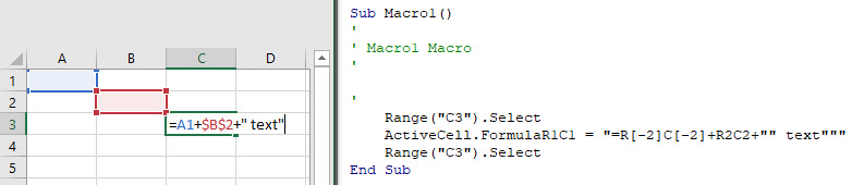
Formula Quotations
If you need to add a quotation (“) within a formula, enter the quotation twice (“”):
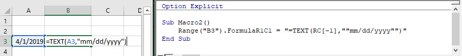
Sub Macro2()
    Range("B3").FormulaR1C1 = "=TEXT(RC[-1],""mm/dd/yyyy"")"
End Sub
A single quotation (“) signifies to VBA the end of a string of text. Whereas a double quotation (“”) is treated like a quotation within the string of text.
Similarly, use 3 quotation marks (“””) to surround a string with a quotation mark (“)
MsgBox """Use 3 to surround a string with quotes"""
' This will print <"Use 3 to surround a string with quotes"> immediate window
Assign Cell Formula to String Variable
We can read the formula in a given cell or range and assign it to a string variable:
'Assign Cell Formula to Variable
Dim strFormula as String
strFormula = Range("B1").Formula
Different Ways to Add Formulas to a Cell
Here are a few more examples for how to assign a formula to a cell:
- Directly Assign Formula
- Define a String Variable Containing the Formula
- Use Variables to Create Formula
Sub MoreFormulaExamples ()
' Alternate ways to add SUM formula
' to cell B1
'
  Dim strFormula as String
  Dim cell as Range
  dim fromRow as long, toRow as long

  Set cell = Range("B1")

  ' Directly assigning a String
  cell.Formula = "=SUM(A1:A10)"

  ' Storing string to a variable
  ' and assigning to "Formula" property
  strFormula = "=SUM(A1:A10)"
  cell.Formula = strFormula

  ' Using variables to build a string
  ' and assigning it to "Formula" property
  fromRow = 1
  toRow   = 10
  strFormula = "=SUM(A" & fromValue & ":A" & toValue & ")
  cell.Formula = strFormula
End Sub
Refresh Formulas
As a reminder, to refresh formulas, you can use the Calculate command:
CalculateTo refresh single formula, range, or entire worksheet use .Calculate instead:
Sheets("Sheet1").Range("a1:a10").Calculate| title | keywords | f1_keywords | ms.prod | ms.assetid | ms.date | ms.localizationpriority |
|---|---|---|---|---|---|---|
|
Cell Formulas |
excel |
??? |
12/10/2019 |
medium |
Range.Formula and Range.Formula2 are two different ways of representing the logic in the formula. They can be thought of a 2 dialects of Excel’s formula language.
Excel has always supported two types of formula evaluation: Implicitly Intersection Evaluation («IIE») and Array Evaluation («AE»). Before the introduction of Dynamic Arrays, IIE was the default for cell formulas, while AE was used everywhere else (Conditional Formatting, Data Validation, CSE Array formulas, etc).
The primary difference between the two forms of Evaluation was how they behaved when a multi celled range (e.g. A1:A10) was passed to a function that expected a single value:
- IIE would choose the cell on the same row or column as the formula. This operation is referred to as «implicit intersection».
- AE would call the function with each cell in the multi celled range and return an array of results. This operation is referred to as «lifting».
When Range.Formula is used to set a cell’s formula, IIE is used for evaluation.
With the introduction of Dyanamic Arrays («DA»), Excel now supports returning multiple values to the grid and AE is now the default. AE formula’s can be set/read using Range.Formula2 which supersedes Range.Formula. However, to facilitate backcompatiblity, Range.Formula is still supported and will continue to set/return IIE formulas. Formula’s set using Range.Formula will trigger implicit intersection and can never spill. Formula read using Range.Formula will continue to be silent on where Implicit Intersection occurs.
Range.Formula effectively reports what would be presented in the formula bar in Pre-DA Excel, while Range.Formula2 reports the formula reported by the formula bar in DA Excel.
Excel automatically translates between these two formula variations, so either can be read and set. To facilitate the translation from Range.Formula (using IIE) to Range.Formula2 (AE), Excel will indicate where implicit intersection could occur using the new implicit intersection operator @. Likewise, to facilitate the translation from Range.Formula2 (using AE) to Range.Formula (using IIE) Excel will remove @ operators that would be performed silently. Often there is no difference between the two.
Translating from Range.Formula to Range.Formula2
This example shows the outcome of setting Range.Formula and then retrieving Range.Formula2
Dim cell As Range
Dim str As String

Set cell = Worksheets("Sheet1").Cells(2, 1)
ArrayOfFormulas = Array("=SQRT(A1)", "=SQRT(A1:A4)")

For i = LBound(ArrayOfFormulas) To UBound(ArrayOfFormulas)
 cell.Formula = ArrayOfFormulas(i)
 str = "Wrote Range.Formula:" & vbCr & cell.Formula & _
    vbCr & vbCr & _
    "Read Range.Formula2:" & vbCr & cell.Formula2
 MsgBox (str)
Next i
| Write Range.Formula | Read Range.Formula2 | Notes |
|---|---|---|
| =SQRT(A1) | =SQRT(A1) | Identical because no implicit intersection could occur |
| =SQRT(A1:A4) | =SQRT(@A1:A4) | SQRT expects a single value but is given an multi celled range. This will trigger implicit intersection in IIE, therefor the translation to AE calls out where implicit intersection could occur using the @ operator |
Translating from Range.Formula2 to Range.Formula
Formula set using Range.Formula2 Excel use AE. On file save, DA Excel examines the formulas in the workbook to determine if they would calculate the same in AE and IIE. If they do, to improve backcompatibility, Excel may save it as an IIE to reduce the number of Array formulas seen by Pre DA versions of Excel. You can test whether the formula will be saved to file as an array formula using Range.SavedAsArray()
Dim cell As Range
Dim str As String

Set cell = Worksheets("Sheet1").Cells(2, 1)
ArrayOfFormulas = Array("=SQRT(A1)", "=SQRT(@A1:A4)", "=SQRT(A1:A4)", "=SQRT(A1:A4)+SQRT(@A1:A4)")

For i = LBound(ArrayOfFormulas) To UBound(ArrayOfFormulas)
 cell.Formula2 = ArrayOfFormulas(i)
 str = "Wrote Range.Formula2:" & vbCr & cell.Formula2 & _
    vbCr & vbCr & _
    "Read Range.Formula:" & vbCr & cell.Formula & _
    vbCr & vbCr & _
    "Read Range.IsSavedAsArray:" & vbCr & cell.SavedAsArray
 MsgBox (str)
Next i
| Write Range.Formula2 | Read Range.Formula | Read Range.SavedAsArray | Notes |
|---|---|---|---|
| =SQRT(A1) | =SQRT(A1) | FALSE | SQRT expects a single value, A1 is a single value. Therefor no variance between IIE and AE. Save as IIE and remove any @’s |
| =SQRT(@A1:A4) | =SQRT(A1:A4) | FALSE | SQRT expects a single value, @A1:A4 is a single value. Therefor no variance between IIE and AE. Save as IIE and remove any @’s |
| =SQRT(A1:A4) | =SQRT(A1:A4) | TRUE | SQRT expects a single value, A1:A4 is a multicell range. IIE and AE could vary therefor save as array |
| =SQRT(A1:A4)+ SQRT(@A1:A4) | =SQRT(A1:A4)+ SQRT(@A1:A4) | TRUE | The first SQRT expects a single value, A1:A4 is a multicell range. IIE and AE could vary therefor save as array |
Best Practice
If targeting DA version of Excel, you should use Range.Formula2 in preference to Range.Formula.
If targeting Pre and Post DA version of Excel, you should continue to use Range.Formula. If however you want tight control over the appearance of the formula the users formula bar, you should detect whether .Formula2 is supported and, if so, use .Formula2 otherwise use .Formula
Notes
OfficeJS does not include Range.Formula2. Instead Range.Formula always reports what is present in the formula bar. As a newer language with the ability for addins to quickly deploy updates, developers are encouraged to update their addins if they encounter any compatibility issues between AE to IIE.
[!includeSupport and feedback]
It is possible to use Excel’s ready-to-use formulas through VBA programming. These are properties that can be used with Range or Cells.
VBA Formula
Formula adds predefined Excel formulas to the worksheet. These formulas should be written in English even if you have a language pack installed.
    Range("F2").Formula = "=SUM(B2:C7)"
    Range("F3").Formula = "=SUM($B$2:$C$7)"
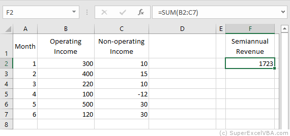
Do not worry if the language of your Excel is not English because, as in the example, it will do the translation to the spreadsheet automatically.
Multiple formulas
You can insert multiple formulas at the same time using the Formula property. To do this, simply define a Range object that is larger than a single cell, and the predefined formula will be «dragged» across the range.
«Dragging» manually:
«Dragging» by VBA:
Range("D2:D7").Formula = "=SUM(B2:C2)"
Another way to perform the same action would be using FillDown method.
    Range("D2").Formula = "=SUM(B2:C2)"
    Range("D2:D7").FillDown
VBA FormulaLocal
FormulaLocal adds predefined Excel formulas to the worksheet. These formulas, however, should be written in the local language of Excel (in the case of Brazil, in Portuguese).
Range("F2").FormulaLocal = "=SOMA(B2:C7)"
Just as the Formula property, FormulaLocal can be used to make multiple formulas.
VBA FormulaR1C1
FormulaR1C1, as well as Formula and FormulaLocal, also adds pre-defined Excel formulas to the spreadsheet; however, the use of relative and absolute notations have different rules. The formula used must be written in English.
FormulaR1C1 is the way to use Excel’s ready-to-use formulas in VBA by easily integrating them into loops and counting variables.
In the notations:
- R refers to rows, in the case of vertical displacement
- C refers to columns, in the case of horizontal displacement
- N symbolizes an integer that indicates how much must be shifted in number of rows and/or columns
- Relative notation: Use as reference the Range that called it
The format of the relative formula is: R[N]C[N]:R[N]C[N].
    Range("F2").FormulaR1C1 = "=SUM(R[0]C[-4]:R[5]C[-3])" 'Equals the bottom row
    Range("F2").FormulaR1C1 = "=SUM(RC[-4]:R[5]C[-3])"
When N is omitted, the value 0 is assumed.
In the example, RC[-4]:R[5]C[-3] results in «B2: C7». These cells are obtained by: receding 4 columns to the left RC[-4] from Range(«F2») to obtain «B2»; and 5 lines down and 3 columns to the left R[5]C[-3] from Range(«F2») to obtain «C7».
- Absolute notation: Use the start of the spreadsheet as a reference
The format of the relative formula is: RNCN:RNCN.
Range("F2").FormulaR1C1 = "=SUM(R2C2:R7C3)" 'Results in "$B$2:$C$7"
N negative can only be used in relative notation.
The two notations (relative and absolute) can be merged.
Range("F2").FormulaR1C1 = "=SUM(RC[-4]:R7C3)" 'Results in "B2:$C$7"
VBA WorksheetFunction
Excel formulas can also be accessed by object WorksheetFunction methods.
Range("F2") = WorksheetFunction.Sum(Range("B2:C7"))
Excel formulas can also be accessed similarly to functions created in VBA.
The formulas present in the WorksheetFunction object are all in English.
One of the great advantages of accessing Excel formulas this way is to be able to use them more easily in the VBA environment.
    MsgBox (WorksheetFunction.Sum(3, 4, 5))
    Expense=4
    MsgBox (WorksheetFunction.Sum(3, 4, 5,-Expense))
To list the available Excel formulas in this format, simply type WorksheetFunction. that automatically an option menu with all formulas will appear:
Consolidating Your Learning
Suggested Exercise
SuperExcelVBA.com is learning website. Examples might be simplified to improve reading and basic understanding. Tutorials, references, and examples are constantly reviewed to avoid errors, but we cannot warrant full correctness of all content. All Rights Reserved.
Excel ® is a registered trademark of the Microsoft Corporation.
© 2023 SuperExcelVBA | ABOUT
![]()
“It is a capital mistake to theorize before one has data”- Sir Arthur Conan Doyle
This post covers everything you need to know about using Cells and Ranges in VBA. You can read it from start to finish as it is laid out in a logical order. If you prefer you can use the table of contents below to go to a section of your choice.
Topics covered include Offset property, reading values between cells, reading values to arrays and formatting cells.
A Quick Guide to Ranges and Cells
| Function | Takes | Returns | Example | Gives |
|---|---|---|---|---|
|
Range |
cell address | multiple cells | .Range(«A1:A4») | $A$1:$A$4 |
| Cells | row, column | one cell | .Cells(1,5) | $E$1 |
| Offset | row, column | multiple cells | Range(«A1:A2») .Offset(1,2) |
$C$2:$C$3 |
| Rows | row(s) | one or more rows | .Rows(4) .Rows(«2:4») |
$4:$4 $2:$4 |
| Columns | column(s) | one or more columns | .Columns(4) .Columns(«B:D») |
$D:$D $B:$D |
Download the Code
The Webinar
If you are a member of the VBA Vault, then click on the image below to access the webinar and the associated source code.
(Note: Website members have access to the full webinar archive.)

Introduction
This is the third post dealing with the three main elements of VBA. These three elements are the Workbooks, Worksheets and Ranges/Cells. Cells are by far the most important part of Excel. Almost everything you do in Excel starts and ends with Cells.
Generally speaking, you do three main things with Cells
- Read from a cell.
- Write to a cell.
- Change the format of a cell.
Excel has a number of methods for accessing cells such as Range, Cells and Offset.These can cause confusion as they do similar things and can lead to confusion
In this post I will tackle each one, explain why you need it and when you should use it.
Let’s start with the simplest method of accessing cells – using the Range property of the worksheet.
Important Notes
I have recently updated this article so that is uses Value2.
You may be wondering what is the difference between Value, Value2 and the default:
' Value2
Range("A1").Value2 = 56

' Value
Range("A1").Value = 56

' Default uses value
Range("A1") = 56
Using Value may truncate number if the cell is formatted as currency. If you don’t use any property then the default is Value.
It is better to use Value2 as it will always return the actual cell value(see this article from Charle Williams.)
The Range Property
The worksheet has a Range property which you can use to access cells in VBA. The Range property takes the same argument that most Excel Worksheet functions take e.g. “A1”, “A3:C6” etc.
The following example shows you how to place a value in a cell using the Range property.
' https://excelmacromastery.com/
Public Sub WriteToCell()

    ' Write number to cell A1 in sheet1 of this workbook
    ThisWorkbook.Worksheets("Sheet1").Range("A1").Value2 = 67

    ' Write text to cell A2 in sheet1 of this workbook
    ThisWorkbook.Worksheets("Sheet1").Range("A2").Value2 = "John Smith"

    ' Write date to cell A3 in sheet1 of this workbook
    ThisWorkbook.Worksheets("Sheet1").Range("A3").Value2 = #11/21/2017#

End Sub
As you can see Range is a member of the worksheet which in turn is a member of the Workbook. This follows the same hierarchy as in Excel so should be easy to understand. To do something with Range you must first specify the workbook and worksheet it belongs to.
For the rest of this post I will use the code name to reference the worksheet.

The following code shows the above example using the code name of the worksheet i.e. Sheet1 instead of ThisWorkbook.Worksheets(“Sheet1”).
' https://excelmacromastery.com/
Public Sub UsingCodeName()

    ' Write number to cell A1 in sheet1 of this workbook
    Sheet1.Range("A1").Value2 = 67

    ' Write text to cell A2 in sheet1 of this workbook
    Sheet1.Range("A2").Value2 = "John Smith"

    ' Write date to cell A3 in sheet1 of this workbook
    Sheet1.Range("A3").Value2 = #11/21/2017#

End Sub
You can also write to multiple cells using the Range property
' https://excelmacromastery.com/
Public Sub WriteToMulti()

    ' Write number to a range of cells
    Sheet1.Range("A1:A10").Value2 = 67

    ' Write text to multiple ranges of cells
    Sheet1.Range("B2:B5,B7:B9").Value2 = "John Smith"

End Sub
You can download working examples of all the code from this post from the top of this article.
The Cells Property of the Worksheet
The worksheet object has another property called Cells which is very similar to range. There are two differences
- Cells returns a range of one cell only.
- Cells takes row and column as arguments.
The example below shows you how to write values to cells using both the Range and Cells property
' https://excelmacromastery.com/
Public Sub UsingCells()

    ' Write to A1
    Sheet1.Range("A1").Value2 = 10
    Sheet1.Cells(1, 1).Value2  = 10

    ' Write to A10
    Sheet1.Range("A10").Value2 = 10
    Sheet1.Cells(10, 1).Value2  = 10

    ' Write to E1
    Sheet1.Range("E1").Value2 = 10
    Sheet1.Cells(1, 5).Value2  = 10

End Sub
You may be wondering when you should use Cells and when you should use Range. Using Range is useful for accessing the same cells each time the Macro runs.
For example, if you were using a Macro to calculate a total and write it to cell A10 every time then Range would be suitable for this task.
Using the Cells property is useful if you are accessing a cell based on a number that may vary. It is easier to explain this with an example.
In the following code, we ask the user to specify the column number. Using Cells gives us the flexibility to use a variable number for the column.
' https://excelmacromastery.com/
Public Sub WriteToColumn()

    Dim UserCol As Integer

    ' Get the column number from the user
    UserCol = Application.InputBox(" Please enter the column...", Type:=1)

    ' Write text to user selected column
    Sheet1.Cells(1, UserCol).Value2 = "John Smith"

End Sub
In the above example, we are using a number for the column rather than a letter.
To use Range here would require us to convert these values to the letter/number cell reference e.g. “C1”. Using the Cells property allows us to provide a row and a column number to access a cell.
Sometimes you may want to return more than one cell using row and column numbers. The next section shows you how to do this.
Using Cells and Range together
As you have seen you can only access one cell using the Cells property. If you want to return a range of cells then you can use Cells with Ranges as follows
' https://excelmacromastery.com/
Public Sub UsingCellsWithRange()

    With Sheet1
        ' Write 5 to Range A1:A10 using Cells property
        .Range(.Cells(1, 1), .Cells(10, 1)).Value2 = 5

        ' Format Range B1:Z1 to be bold
        .Range(.Cells(1, 2), .Cells(1, 26)).Font.Bold = True

    End With

End Sub
As you can see, you provide the start and end cell of the Range. Sometimes it can be tricky to see which range you are dealing with when the value are all numbers. Range has a property called Address which displays the letter/ number cell reference of any range. This can come in very handy when you are debugging or writing code for the first time.
In the following example we print out the address of the ranges we are using:
' https://excelmacromastery.com/
Public Sub ShowRangeAddress()

    ' Note: Using underscore allows you to split up lines of code
    With Sheet1

        ' Write 5 to Range A1:A10 using Cells property
        .Range(.Cells(1, 1), .Cells(10, 1)).Value2 = 5
        Debug.Print "First address is : " _
            + .Range(.Cells(1, 1), .Cells(10, 1)).Address

        ' Format Range B1:Z1 to be bold
        .Range(.Cells(1, 2), .Cells(1, 26)).Font.Bold = True
        Debug.Print "Second address is : " _
            + .Range(.Cells(1, 2), .Cells(1, 26)).Address

    End With

End Sub
In the example I used Debug.Print to print to the Immediate Window. To view this window select View->Immediate Window(or Ctrl G)


You can download all the code for this post from the top of this article.
The Offset Property of Range
Range has a property called Offset. The term Offset refers to a count from the original position. It is used a lot in certain areas of programming. With the Offset property you can get a Range of cells the same size and a certain distance from the current range. The reason this is useful is that sometimes you may want to select a Range based on a certain condition. For example in the screenshot below there is a column for each day of the week. Given the day number(i.e. Monday=1, Tuesday=2 etc.) we need to write the value to the correct column.

We will first attempt to do this without using Offset.
' https://excelmacromastery.com/
' This sub tests with different values
Public Sub TestSelect()

    ' Monday
    SetValueSelect 1, 111.21
    ' Wednesday
    SetValueSelect 3, 456.99
    ' Friday
    SetValueSelect 5, 432.25
    ' Sunday
    SetValueSelect 7, 710.17

End Sub

' Writes the value to a column based on the day
Public Sub SetValueSelect(lDay As Long, lValue As Currency)

    Select Case lDay
        Case 1: Sheet1.Range("H3").Value2 = lValue
        Case 2: Sheet1.Range("I3").Value2 = lValue
        Case 3: Sheet1.Range("J3").Value2 = lValue
        Case 4: Sheet1.Range("K3").Value2 = lValue
        Case 5: Sheet1.Range("L3").Value2 = lValue
        Case 6: Sheet1.Range("M3").Value2 = lValue
        Case 7: Sheet1.Range("N3").Value2 = lValue
    End Select

End Sub
As you can see in the example, we need to add a line for each possible option. This is not an ideal situation. Using the Offset Property provides a much cleaner solution
' https://excelmacromastery.com/
' This sub tests with different values
Public Sub TestOffset()

    DayOffSet 1, 111.01
    DayOffSet 3, 456.99
    DayOffSet 5, 432.25
    DayOffSet 7, 710.17

End Sub

Public Sub DayOffSet(lDay As Long, lValue As Currency)

    ' We use the day value with offset specify the correct column
    Sheet1.Range("G3").Offset(, lDay).Value2 = lValue

End Sub
As you can see this solution is much better. If the number of days in increased then we do not need to add any more code. For Offset to be useful there needs to be some kind of relationship between the positions of the cells. If the Day columns in the above example were random then we could not use Offset. We would have to use the first solution.
One thing to keep in mind is that Offset retains the size of the range. So .Range(“A1:A3”).Offset(1,1) returns the range B2:B4. Below are some more examples of using Offset
' https://excelmacromastery.com/
Public Sub UsingOffset()

    ' Write to B2 - no offset
    Sheet1.Range("B2").Offset().Value2 = "Cell B2"

    ' Write to C2 - 1 column to the right
    Sheet1.Range("B2").Offset(, 1).Value2 = "Cell C2"

    ' Write to B3 - 1 row down
    Sheet1.Range("B2").Offset(1).Value2 = "Cell B3"

    ' Write to C3 - 1 column right and 1 row down
    Sheet1.Range("B2").Offset(1, 1).Value2 = "Cell C3"

    ' Write to A1 - 1 column left and 1 row up
    Sheet1.Range("B2").Offset(-1, -1).Value2 = "Cell A1"

    ' Write to range E3:G13 - 1 column right and 1 row down
    Sheet1.Range("D2:F12").Offset(1, 1).Value2 = "Cells E3:G13"

End Sub
Using the Range CurrentRegion
CurrentRegion returns a range of all the adjacent cells to the given range.
In the screenshot below you can see the two current regions. I have added borders to make the current regions clear.

A row or column of blank cells signifies the end of a current region.
You can manually check the CurrentRegion in Excel by selecting a range and pressing Ctrl + Shift + *.
If we take any range of cells within the border and apply CurrentRegion, we will get back the range of cells in the entire area.
For example
Range(“B3”).CurrentRegion will return the range B3:D14
Range(“D14”).CurrentRegion will return the range B3:D14
Range(“C8:C9”).CurrentRegion will return the range B3:D14
and so on
How to Use
We get the CurrentRegion as follows
' Current region will return B3:D14 from above example
Dim rg As Range
Set rg = Sheet1.Range("B3").CurrentRegion
Read Data Rows Only
Read through the range from the second row i.e.skipping the header row
' Current region will return B3:D14 from above example
Dim rg As Range
Set rg = Sheet1.Range("B3").CurrentRegion

' Start at row 2 - row after header
Dim i As Long
For i = 2 To rg.Rows.Count
    ' current row, column 1 of range
    Debug.Print rg.Cells(i, 1).Value2
Next i
Remove Header
Remove header row(i.e. first row) from the range. For example if range is A1:D4 this will return A2:D4
' Current region will return B3:D14 from above example
Dim rg As Range
Set rg = Sheet1.Range("B3").CurrentRegion

' Remove Header
Set rg = rg.Resize(rg.Rows.Count - 1).Offset(1)

' Start at row 1 as no header row
Dim i As Long
For i = 1 To rg.Rows.Count
    ' current row, column 1 of range
    Debug.Print rg.Cells(i, 1).Value2
Next i
Using Rows and Columns as Ranges
If you want to do something with an entire Row or Column you can use the Rows or Columns property of the Worksheet. They both take one parameter which is the row or column number you wish to access
' https://excelmacromastery.com/
Public Sub UseRowAndColumns()

    ' Set the font size of column B to 9
    Sheet1.Columns(2).Font.Size = 9

    ' Set the width of columns D to F
    Sheet1.Columns("D:F").ColumnWidth = 4

    ' Set the font size of row 5 to 18
    Sheet1.Rows(5).Font.Size = 18

End Sub
Using Range in place of Worksheet
You can also use Cells, Rows and Columns as part of a Range rather than part of a Worksheet. You may have a specific need to do this but otherwise I would avoid the practice. It makes the code more complex. Simple code is your friend. It reduces the possibility of errors.
The code below will set the second column of the range to bold. As the range has only two rows the entire column is considered B1:B2
' https://excelmacromastery.com/
Public Sub UseColumnsInRange()

    ' This will set B1 and B2 to be bold
    Sheet1.Range("A1:C2").Columns(2).Font.Bold = True

End Sub
You can download all the code for this post from the top of this article.
Reading Values from one Cell to another
In most of the examples so far we have written values to a cell. We do this by placing the range on the left of the equals sign and the value to place in the cell on the right. To write data from one cell to another we do the same. The destination range goes on the left and the source range goes on the right.
The following example shows you how to do this:
' https://excelmacromastery.com/
Public Sub ReadValues()

    ' Place value from B1 in A1
    Sheet1.Range("A1").Value2 = Sheet1.Range("B1").Value2

    ' Place value from B3 in sheet2 to cell A1
    Sheet1.Range("A1").Value2 = Sheet2.Range("B3").Value2

    ' Place value from B1 in cells A1 to A5
    Sheet1.Range("A1:A5").Value2 = Sheet1.Range("B1").Value2

    ' You need to use the "Value" property to read multiple cells
    Sheet1.Range("A1:A5").Value2 = Sheet1.Range("B1:B5").Value2

End Sub
As you can see from this example it is not possible to read from multiple cells. If you want to do this you can use the Copy function of Range with the Destination parameter
' https://excelmacromastery.com/
Public Sub CopyValues()

    ' Store the copy range in a variable
    Dim rgCopy As Range
    Set rgCopy = Sheet1.Range("B1:B5")

    ' Use this to copy from more than one cell
    rgCopy.Copy Destination:=Sheet1.Range("A1:A5")

    ' You can paste to multiple destinations
    rgCopy.Copy Destination:=Sheet1.Range("A1:A5,C2:C6")

End Sub
The Copy function copies everything including the format of the cells. It is the same result as manually copying and pasting a selection. You can see more about it in the Copying and Pasting Cells section.
Using the Range.Resize Method
When copying from one range to another using assignment(i.e. the equals sign), the destination range must be the same size as the source range.
Using the Resize function allows us to resize a range to a given number of rows and columns.
For example:
' https://excelmacromastery.com/
Sub ResizeExamples()

    ' Prints A1
    Debug.Print Sheet1.Range("A1").Address

    ' Prints A1:A2
    Debug.Print Sheet1.Range("A1").Resize(2, 1).Address

    ' Prints A1:A5
    Debug.Print Sheet1.Range("A1").Resize(5, 1).Address

    ' Prints A1:D1
    Debug.Print Sheet1.Range("A1").Resize(1, 4).Address

    ' Prints A1:C3
    Debug.Print Sheet1.Range("A1").Resize(3, 3).Address

End Sub
When we want to resize our destination range we can simply use the source range size.
In other words, we use the row and column count of the source range as the parameters for resizing:
' https://excelmacromastery.com/
Sub Resize()

    Dim rgSrc As Range, rgDest As Range

    ' Get all the data in the current region
    Set rgSrc = Sheet1.Range("A1").CurrentRegion

      ' Get the range destination
    Set rgDest = Sheet2.Range("A1")
    Set rgDest = rgDest.Resize(rgSrc.Rows.Count, rgSrc.Columns.Count)

    rgDest.Value2 = rgSrc.Value2

End Sub
We can do the resize in one line if we prefer:
' https://excelmacromastery.com/
Sub ResizeOneLine()

    Dim rgSrc As Range

    ' Get all the data in the current region
    Set rgSrc = Sheet1.Range("A1").CurrentRegion

    With rgSrc
        Sheet2.Range("A1").Resize(.Rows.Count, .Columns.Count).Value2 = .Value2
    End With

End Sub
Reading Values to variables
We looked at how to read from one cell to another. You can also read from a cell to a variable. A variable is used to store values while a Macro is running. You normally do this when you want to manipulate the data before writing it somewhere. The following is a simple example using a variable. As you can see the value of the item to the right of the equals is written to the item to the left of the equals.
' https://excelmacromastery.com/
Public Sub UseVariables()

    ' Create
    Dim number As Long

    ' Read number from cell
    number = Sheet1.Range("A1").Value2

    ' Add 1 to value
    number = number + 1

    ' Write new value to cell
    Sheet1.Range("A2").Value2 = number

End Sub
To read text to a variable you use a variable of type String:
' https://excelmacromastery.com/
Public Sub UseVariableText()

    ' Declare a variable of type string
    Dim text As String

    ' Read value from cell
    text = Sheet1.Range("A1").Value2

    ' Write value to cell
    Sheet1.Range("A2").Value2 = text

End Sub
You can write a variable to a range of cells. You just specify the range on the left and the value will be written to all cells in the range.
' https://excelmacromastery.com/
Public Sub VarToMulti()

    ' Read value from cell
    Sheet1.Range("A1:B10").Value2 = 66

End Sub
You cannot read from multiple cells to a variable. However you can read to an array which is a collection of variables. We will look at doing this in the next section.
How to Copy and Paste Cells
If you want to copy and paste a range of cells then you do not need to select them. This is a common error made by new VBA users.
Note: We normally use Range.Copy when we want to copy formats, formulas, validation. If we want to copy values it is not the most efficient method.
I have written a complete guide to copying data in Excel VBA here.
You can simply copy a range of cells like this:
Range("A1:B4").Copy Destination:=Range("C5")
Using this method copies everything – values, formats, formulas and so on. If you want to copy individual items you can use the PasteSpecial property of range.
It works like this
Range("A1:B4").Copy
Range("F3").PasteSpecial Paste:=xlPasteValues
Range("F3").PasteSpecial Paste:=xlPasteFormats
Range("F3").PasteSpecial Paste:=xlPasteFormulas
The following table shows a full list of all the paste types
| Paste Type |
|---|
| xlPasteAll |
| xlPasteAllExceptBorders |
| xlPasteAllMergingConditionalFormats |
| xlPasteAllUsingSourceTheme |
| xlPasteColumnWidths |
| xlPasteComments |
| xlPasteFormats |
| xlPasteFormulas |
| xlPasteFormulasAndNumberFormats |
| xlPasteValidation |
| xlPasteValues |
| xlPasteValuesAndNumberFormats |
Reading a Range of Cells to an Array
You can also copy values by assigning the value of one range to another.
Range("A3:Z3").Value2 = Range("A1:Z1").Value2
The value of range in this example is considered to be a variant array. What this means is that you can easily read from a range of cells to an array. You can also write from an array to a range of cells. If you are not familiar with arrays you can check them out in this post.
The following code shows an example of using an array with a range:
' https://excelmacromastery.com/
Public Sub ReadToArray()

    ' Create dynamic array
    Dim StudentMarks() As Variant

    ' Read 26 values into array from the first row
    StudentMarks = Range("A1:Z1").Value2

    ' Do something with array here

    ' Write the 26 values to the third row
    Range("A3:Z3").Value2 = StudentMarks

End Sub
Keep in mind that the array created by the read is a 2 dimensional array. This is because a spreadsheet stores values in two dimensions i.e. rows and columns
Going through all the cells in a Range
Sometimes you may want to go through each cell one at a time to check value.
You can do this using a For Each loop shown in the following code
' https://excelmacromastery.com/
Public Sub TraversingCells()

    ' Go through each cells in the range
    Dim rg As Range
    For Each rg In Sheet1.Range("A1:A10,A20")
        ' Print address of cells that are negative
        If rg.Value < 0 Then
            Debug.Print rg.Address + " is negative."
        End If
    Next

End Sub
You can also go through consecutive Cells using the Cells property and a standard For loop.
The standard loop is more flexible about the order you use but it is slower than a For Each loop.
' https://excelmacromastery.com/
Public Sub TraverseCells()

    ' Go through cells from A1 to A10
    Dim i As Long
    For i = 1 To 10
        ' Print address of cells that are negative
        If Range("A" & i).Value < 0 Then
            Debug.Print Range("A" & i).Address + " is negative."
        End If
    Next

    ' Go through cells in reverse i.e. from A10 to A1
    For i = 10 To 1 Step -1
        ' Print address of cells that are negative
        If Range("A" & i) < 0 Then
            Debug.Print Range("A" & i).Address + " is negative."
        End If
    Next

End Sub
Formatting Cells
Sometimes you will need to format the cells the in spreadsheet. This is actually very straightforward. The following example shows you various formatting you can add to any range of cells
' https://excelmacromastery.com/
Public Sub FormattingCells()

    With Sheet1

        ' Format the font
        .Range("A1").Font.Bold = True
        .Range("A1").Font.Underline = True
        .Range("A1").Font.Color = rgbNavy

        ' Set the number format to 2 decimal places
        .Range("B2").NumberFormat = "0.00"
        ' Set the number format to a date
        .Range("C2").NumberFormat = "dd/mm/yyyy"
        ' Set the number format to general
        .Range("C3").NumberFormat = "General"
        ' Set the number format to text
        .Range("C4").NumberFormat = "Text"

        ' Set the fill color of the cell
        .Range("B3").Interior.Color = rgbSandyBrown

        ' Format the borders
        .Range("B4").Borders.LineStyle = xlDash
        .Range("B4").Borders.Color = rgbBlueViolet

    End With

End Sub
Main Points
The following is a summary of the main points
- Range returns a range of cells
- Cells returns one cells only
- You can read from one cell to another
- You can read from a range of cells to another range of cells.
- You can read values from cells to variables and vice versa.
- You can read values from ranges to arrays and vice versa
- You can use a For Each or For loop to run through every cell in a range.
- The properties Rows and Columns allow you to access a range of cells of these types
What’s Next?
Free VBA Tutorial If you are new to VBA or you want to sharpen your existing VBA skills then why not try out the The Ultimate VBA Tutorial.
Related Training: Get full access to the Excel VBA training webinars and all the tutorials.
(NOTE: Planning to build or manage a VBA Application? Learn how to build 10 Excel VBA applications from scratch.)