
Not every user will have a need for random numbers in Excel. Most people work with fixed numbers and formulas and may have no need for random numbers to appear in their reports.
However, a random number generator does have a huge use when working with different scenarios on a set of data or when performing various statistical analyses.
A financial model may use a stochastic simulation that is dependent on probabilities. The model may need to be run thousands of times, but with the random number generator providing the parameters of each simulation.
Whatever your need for random numbers, Excel has several ways to generate them.
In this post, I’ll show you all the methods you can use to insert random numbers into your workbooks.
Generate Random Numbers with the RAND function
The first way I will show you is the easiest way to generate random values in Excel.
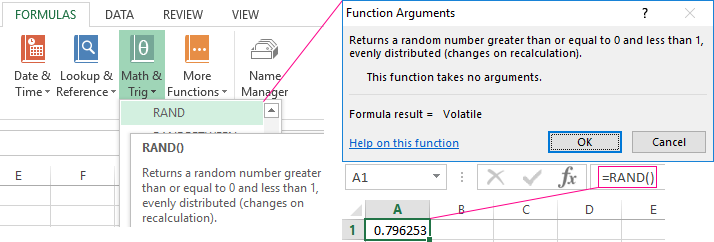
There is a very simple RAND function that requires no parameters and will generate a random number between 0 and 1.
Syntax for the RAND Function
= RAND ( )This function has no required or optional arguments. The function is always entered with an empty set of parenthesis.
This function will generate a decimal random number between 0 and 1, but not including 0 or 1.
Repeated values are possible but unlikely since the RAND function produces numbers from a continuous range of numbers.
The values that are returned will follow a uniform distribution. This means that any number between 0 and 1 is equally likely to be returned.
Generate Random Numbers Between Any Two Numbers
A decimal number between 0 and 1 may not be too useful if you need numbers between 1 and 10.
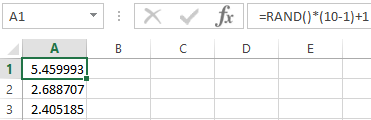
But you can use a simple formula involving the RAND function to generate random numbers between any two numbers.
= RAND ( ) * ( Y - X ) + XIn general, you can create a random number between X and Y by using the above formula.
= RAND ( ) * 9 + 1For example, to generate numbers between 1 and 10 you can use the above formula.
This multiplies the random number generated by 9 and then adds 1 to it. This will produce decimal numbers between 1 and 10.
Generate Random Integer Numbers Between Any Two Numbers
Another possible need you may encounter is to generate random whole numbers between two given numbers. This can also be done using a simple formula.
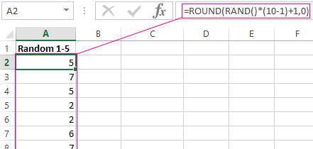
= ROUND ( RAND ( ) * ( Y - X ) + X, 0 )In general, you can use the above formula to generate random integer numbers between two values X and Y.
= ROUND ( RAND ( ) * 9 + 1, 0 )For example, the above formula will create random integer numbers between 1 and 10.
This is the same formula as before, but using the ROUND function to round to zero decimal places.
You can copy this formula down the column on the spreadsheet, and if you keep pressing F9 to re-calculate, you will see various combinations of numbers from 1 to 10.
Since the set of possible numbers is discrete, the random numbers generated may well be duplicated in the list, depending on what the minimum and maximum are of the range.
= ROUND ( RAND ( ) * ( 4 - -3 ) + -3, 0 )This also works for producing negative numbers. Suppose you need to generate random integer numbers between -3 and 4, then the above formula will be what you need.
Multiplying the RAND function by 7 will produce random numbers between 0 and 7. Add -3 to the result and round to zero decimal places, and this will give the range of random numbers of -3 to 4.
Generate Random Numbers using the RANDBETWEEN Function
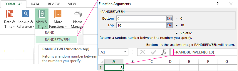
Excel has a useful function for generating random numbers within a range of an upper and lower number.
This is easier to use than using the RAND function as it includes extra operators to arrive at your specific range.
Syntax for the RANDBETWEEN Function
= RANDBETWEEN ( bottom, top )- bottom is the lower range for the values to return.
- top is the upper range for the values to return.
Both of these arguments are required.
This function will produce random integer numbers between the bottom and top values. This function will also return the upper and lower limits as possible values as it’s not strictly between in this function.
Example with the RANDBETWEEN Function
= RANDBETWEEN ( -3, 4 )For example, if you wanted random numbers between -3 and 4, as in the previous example, you can use the above formula.
Note that the RANDBETWEEN function can only produce integer numbers. There is no way of making the function produce decimal numbers. However, it is considerably less complicated than using the RAND function with operators to achieve the same result.
Generate Random Numbers with the RANDARRAY Function
Usually, it’s the case that you don’t want just a single random value but an entire set of random values.
The RANDARRAY function is the perfect solution for this.
It will populate a range of cells with an array of random numbers, which can be very powerful.
This function is only available on the Microsoft 365 version of Excel.
Syntax for the RANDARRAY Function
= RANDARRAY ( [rows], [columns], [min], [max], [whole_number] )- Rows is the number of rows to return.
- Columns is the number of columns to return.
- Min is the minimum value for the random numbers.
- Max is the maximum value for the random numbers.
- Whole_Number is TRUE to return whole numbers, and FALSE to return decimal numbers.
All the arguments are optional for this function.
If no parameters are included, you will get a single random number with decimal places, in the same way as the RAND function.
Example with the RANDARRAY Function
= RANDARRAY ( 4, 3, 6, 14, TRUE )To generate an array of 4 rows and 3 columns of whole random numbers between 6 and 14 you can use the above formula.
This will produce an array of values. Notice the blue border around the numbers? These are all produced from a single formula!
Note that the top left-hand corner of the array is always anchored on the cell that the formula is in. Pressing F9 to recalculate the spreadsheet will change all the numbers in the array.
If you do not put a minimum or maximum value, the default of 0 to 1 will be used.
The minimum value must be less than the maximum value otherwise there will be a #VALUE! error.
The array will automatically resize if you change either the rows or columns parameters in the RANDARRAY formula. This is why they’re known as dynamic arrays.
Warning: If there is already data in one of the cells in the output range that you have entered, you will get a #SPILL! error. No data will be overwritten.
Generate Random Numbers with the Analysis Tools Add-In
There is another method that can be used to insert random numbers without using a formula.
You can use an add-in to create random numbers. Excel comes with an Analysis Tool Pak add-in, but you will need to install it before you can use it.
Install the Analysis Toolpak
Here are the steps to install the Analysis Tool Pak add-in.
- Click on the File tab in the ribbon.
- In the lower left-hand pane of the window, scroll down and click on Options. You can also use the keyboard shortcut Alt, F, T from the spreadsheet window to open the Options window.
- In the left-hand pane of the pop-up window, click on Add-Ins.
- At the bottom of the main window displayed, select Excel Add-ins from the dropdown and click on the Go button.
- This will display a pop-up window containing all available add-ins for Excel. Check the box for Analysis ToolPak and then click OK.
- On the Excel ribbon, on the Data tab, there is now an extra group called Analysis with one button called Data Analysis.
Generate Random Numbers with the Analysis Toolpak
Click on the Data Analysis button in the Analysis group.
This will display a pop-up window. Scroll down and select the Random Number Generation option and then click OK.
A new pop-up window will appear where you can enter your parameters to generate the random numbers.
There are several settings that can be customized.
- Number of Variables This is the number of columns of random numbers that you want in your output table. If left blank, then all columns will be filled in the output range that you specify.
- Number of Random Numbers This is the number of rows of random numbers that you want to generate. If left blank, the output range that you specify will be filled.
- Distribution You can select several distribution methods from the drop-down such as uniform or normal distribution. Different options will become available in the Parameters section depending on your selection here.
- Parameters Enter the values to characterize the distribution selected.
- Random Seed This is optional and will be the starting point for the algorithm to produce the random numbers. If you use the same seed again, it will produce the same random numbers. If left blank, it will take the seed value from the timer event.
- Output Range Enter the upper left cell of where the table is to be constructed in the spreadsheet. If you have left the Variables parameter blank, then you will need to specify an entire range. Note that existing data in that range will be overwritten.
- New Worksheet Ply This option will insert a new worksheet within the workbook and will paste the results at Cell A1. Enter a sheet name in the adjacent box, otherwise, a default name will be used.
- New Workbook This will create a new workbook and paste the results into cell A1 in the first sheet.
Press the OK button and Excel will insert the random number according to the selected options.
Notice that unlike the formula methods previously shown, these numbers are hardcoded and will not change when you refresh calculations in the workbook.
Generate Random Numbers with VBA
VBA (Visual Basic for Applications) is the programming language that sits behind the front end of Excel, and this can also be used to generate random numbers.
However, it is more complicated than simply entering a formula into a cell in Excel, and you do need some programming knowledge to use it.
To open the VBA editor, use the Alt + F11 keyboard shortcut.
In the left-hand pane of the window (Project Explorer), you will see the workbooks that are open (including add-ins) and the sheets available.
On the menu at the top of the window, click on Insert and then click on Module. This will add a module window to the current spreadsheet. Paste or add the following code to the module.
Sub RandomNumber()
    MsgBox Rnd()
End Sub
Press F5 to run this, and a message pop-up will appear in Excel with a random number displayed. Press OK and you will return to the code window.
Run the code again and a different random number will be displayed. The random number will be between 0 and 1, but will not include the values of 0 or 1.
You can also give the Rnd function a parameter, which is a seed for the starting point of the algorithm to produce the random numbers.
If the seed value is set to a negative number or zero, then the same random number will be displayed each time.
Using VBA functions, you can emulate all the functionality of the front-end methods that have been covered in this article.
Sub RandomNumberV2()

    MsgBox Round((Rnd() * 7) + 3)
End Sub
For example, if you wanted to generate whole random numbers between 3 and 10, then you would use the following above code.
This code multiplies the random number, by 7, and then adds 3 to it, and then rounds to zero decimal places.
Suppose that you then wanted to display your random numbers in the grid. You can do this with the following code.
Sub RandomNumberSheet()
Dim M As Integer
For M = 1 To 5
    ActiveSheet.Cells(M, 1) = Round((Rnd(10) * 7) + 3, 0)
Next M
End Sub
This code uses a For Next loop to iterate 5 times through the random number calculation and enter the results in a column of cells starting at cell A1.
Remember that any data already there will be overwritten, and there is no warning or undo feature available. Save any previous work beforehand!
Sub RandomNumberV2()
    Randomize (10)
    MsgBox Round((Rnd() * 7) + 3)
End Sub
There is also a VBA function called Randomize. You can use this before the Rnd function to reset the seed value to the timer event, or to any parameter given.
Generate Random Numbers without Duplicates or Repeats
You may well have a situation where you want to generate a range of random numbers, but you do not want to see any duplicate values appearing.
You may want to select 3 random numbers between the numbers from 1 to 10, but where each of the 3 selected numbers is unique.
You could generate random numbers with the RANDBETWEEN function and then use the Excel function Remove Duplicates from the ribbon, but this still may not give you all the numbers required.
There are several possible solutions available.
Solution with RANK.EQ and COUNTIF Functions
If you don’t have access to the RANDARRAY function in Excel, then you can use a combination of RANK.EQ and COUNTIF to get unique random numbers.
You can create your random numbers using RANDBETWEEN and then use a formula in the next column to rank them thereby giving you a randomly sorted sequence from 1 to 10.
= RANDBETWEEN ( 1, 10 )In cell B2, enter the above formula. Copy this formula down so that there are 10 rows of random numbers going down to cell B11.
You will notice that some numbers may be duplicated and some are not shown at all.
You can then use the RANK.EQ function to rank them so as to create a sequence from 1 to 10 but that is sorted randomly.
= RANK.EQ ( B2, $B$2:$B$11 ) + COUNTIF ( $B$2:B2, B2 ) - 1In cell C2, enter the above formula.
Note that there are absolute references used (the $ signs) so that formula references stay fixed as you copy the formula down.
Copy this formula down to cell C11, and this will display all the numbers between 1 and 10, but in random order.
To explain this formula in more depth, it uses two functions RANK.EQ and COUNTIF.
= RANK.EQ ( number, ref, [order] )- Number is the number that we want to find the rank of in the array.
- Ref is the array where we want to search for the number.
- Order is optional and allows you to find the rank in either ascending or descending order. If its omitted then ascending order is used.
The RANK.EQ function returns the rank of a number within an array of numbers.
= COUNTIF ( range, criteria )- Range is the range that is being searched for instances of the criteria.
- Criteria is the value to match within the range.
The COUNTIF function counts the number of cells based on a given criterion. In this case, it is counting how many times a given random number has appeared in the list.
For each random number the RANK.EQ function will determine its ranking position relative to the other random numbers. But if the random numbers contain duplicates, then they will create a tied ranking.
The COUNTIF function will compensate for any ties in the ranking and will add one to the rank for each time the random number has previously appeared.
This creates a unique ranking where ties don’t get the same rank.
Since this rank is based on a set of random numbers the result is the same as randomizing a list of numbers from 1 to 10.
Now, if you only want 5 non-repeating numbers, you only need to take the first 5 from the ranking list.
Solution with VBA
You could also use VBA to generate a string of random numbers from 1 to 10 without duplicates.
Sub RandomNumberNoDuplicates()
Dim M As Integer, Temp As String, RandN As Integer
For M = 1 To 5
Repeat:
    RandN = Round((Rnd(10) * 9) + 1, 0)
    If InStr(Temp, RandN) Then GoTo Repeat
    ActiveSheet.Cells(M, 1) = RandN
    Temp = Temp & RandN & "|"
Next M
End Sub
This code iterates through values from 1 to 5, generating a random number between 1 and 10 each time.
It tests the random number to check if it has already been generated. This is done by concatenating successful numbers into a string and then searching that string to see if the number has already been used.
If it has been found, then it uses the label Repeat to go back and re-generate a new number. This is again tested that it has not already been used. If it is a new number, then it is added to the sheet.
Solution with Dynamic Arrays
If you have dynamic arrays in Excel, then there is a single formula method to avoid repeating values.
Suppose you want to return 5 numbers from the sequence 1 to 10. You want each number selected to be unique.
This can be done using a combination of the SEQUENCE, SORTBY, RANDARRAY, and INDEX functions.
=INDEX(
    SORTBY(
        SEQUENCE(10),
        RANDARRAY(10)
    ),
    SEQUENCE(5)
)
The above formula creates a sequence of numbers from 1 to 10.
It then sorts them in a random order using the SORTBY function and sorting on a column of random numbers generated by the RANDARRAY function. The effect is to sort the sequence in random order.
Now if you want to get 5 random and unique numbers you only need to take the first 5 numbers from the randomly sorted sequence.
This is exactly what the INDEX function does! This part of the formula will return the first 5 numbers from the randomly sorted sequence.
Conclusion
There are several ways to generate random numbers in Excel.
Whether you need whole numbers, decimals, or a range of random numbers with an upper and lower limit, the facility is available. Excel is extremely versatile on this topic.
However, bear in mind that these numbers are pseudo-random numbers generated by an algorithm.
Although the random number generator passes all the tests of randomness, they are not true random numbers.
To be a truly random number, it would have to be driven by a random event happening outside the computer environment.
For most purposes of constructing general simulations and statistical analysis, the Excel random number generator is considered fit for the purpose.
Have you used any of these methods for generating random numbers in Excel? Do you know any other methods? Let me know in the comments below!
About the Author
John is a Microsoft MVP and qualified actuary with over 15 years of experience. He has worked in a variety of industries, including insurance, ad tech, and most recently Power Platform consulting. He is a keen problem solver and has a passion for using technology to make businesses more efficient.
Excel for Microsoft 365 Excel for Microsoft 365 for Mac Excel for the web Excel 2021 Excel 2021 for Mac Excel 2019 Excel 2019 for Mac Excel 2016 Excel 2016 for Mac Excel 2013 Excel 2010 Excel 2007 Excel for Mac 2011 Excel Starter 2010 More…Less
This article describes the formula syntax and usage of the RAND function in Microsoft Excel.
Description
RAND returns an evenly distributed random real number greater than or equal to 0 and less than 1. A new random real number is returned every time the worksheet is calculated.
Syntax
RAND()
The RAND function syntax has no arguments.
Remarks
-
To generate a random real number between a and b, use:
=RAND()*(b-a)+a
-
If you want to use RAND to generate a random number but don’t want the numbers to change every time the cell is calculated, you can enter =RAND() in the formula bar, and then press F9 to change the formula to a random number. The formula will calculate and leave you with just a value.
Example
Copy the example data in the following table, and paste it in cell A1 of a new Excel worksheet. For formulas to show results, select them, press F2, and then press Enter. You can adjust the column widths to see all the data, if needed.
|
Formula |
Description |
Result |
|---|---|---|
|
=RAND() |
A random number greater than or equal to 0 and less than 1 |
varies |
|
=RAND()*100 |
A random number greater than or equal to 0 and less than 100 |
varies |
|
=INT(RAND()*100) |
A random whole number greater than or equal to 0 and less than 100 |
varies |
|
Note: When a worksheet is recalculated by entering a formula or data in a different cell, or by manually recalculating (press F9), a new random number is generated for any formula that uses the RAND function. |
Need more help?
You can always ask an expert in the Excel Tech Community or get support in the Answers community.
See Also
Mersenne Twister algorithm
RANDBETWEEN function
Need more help?
Want more options?
Explore subscription benefits, browse training courses, learn how to secure your device, and more.
Communities help you ask and answer questions, give feedback, and hear from experts with rich knowledge.
We have got a sequence of numbers consisting of virtually independent elements that obey a certain counting distribution. As a rule, it’s a uniform distribution.
There are different ways to generate random numbers in Excel. Let’s view the best of them.
Random Number Function In Excel
- The function RAND() returns a random real number of a uniform distribution. It will be less than 1, and greater than or equal to 0.
- The function RANDBETWEEN returns a random integer number.
Let’s view some examples of their practical application.
Selection of random numbers using RAND
This function doesn’t require arguments.
For example, to generate a random real number in the range 1 to 10, use the following formula: =RAND()*(5-1)+1.
The returned random number is distributed uniformly on the interval [1,10].
Each time the sheet is calculated or the value is changed in any cell within the sheet, a new random number is returned. If you want to save the generated set of numbers, replace the formula with its value.
- Click on the cell containing the random number.
- Select the formula in the formula bar.
- Press F9. Then Enter.
Let us check the uniformity of distribution of the random numbers from the first selection using a distribution bar chart.
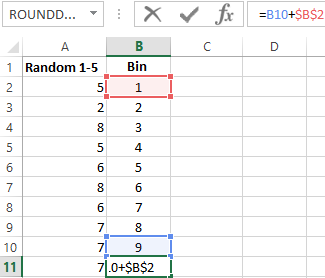
- We round the values that the function =RAND() returns. To do this, we use the function: =ROUND().And fill this formula with the big range: A2:A201.
- Form the ranges to contain the values (bin). The first such range is 0-0.1. For the subsequent ones use the formula =B2+$B$2.
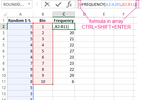
- Determine the frequency of random numbers in range A2:A201. In cell C2 use the array formula:
After input formula, select range C2:C11, press key F2 and press hot keys: CTRL+SHIFT+ENTER. We will execute the formula in the array Excel.
- Form the ranges with the use of the concatenation character (=»[0,0-«&C2&»]»).
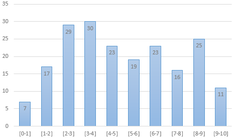
- Build a distribution bar chart for the 200 values obtained with the use of the RAND() function.
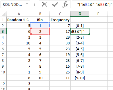
The vertical values represent the frequency. The horizontal ones represent the ranges.
RANDBETWEEN function
The syntax of the RANDBETWEEN function is as follows: (lower limit; upper limit). The first argument must be less than the second. Otherwise, the function will return an error. It is assumed that the limits are integers. The formula discards the fractional part.
An example of the function’s application:
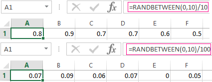
Random numbers with an accuracy of 0.1 and 0.01:
How To Create Random Number Generator In Excel
Let’s create a random number generator that generates values from a certain range. Use a formula of the following form:
The formula randomly selects any of the numbers in the range A1:A10.
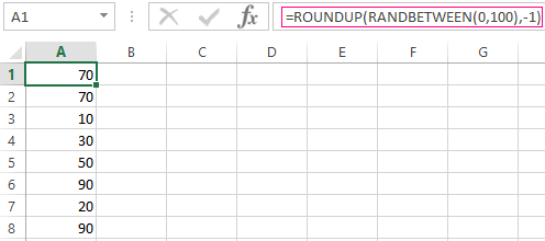
Let’s create a random number generator in the range 0-100, with a step of 10.
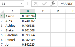
It’s required to select 2 random text values from the list. Using the RAND() function, let’s match the text values in the range A1:A7 with random numbers.
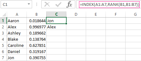
Use the =INDEX function to select two random text values from the initial list.
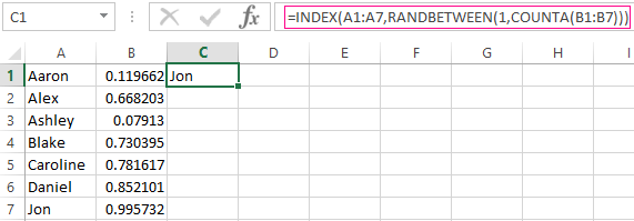
To select one random value from the list, apply the following formula:
Generator Of Standard Distribution Random Numbers
The RAND and RANDBETWEEN functions return random numbers with a single distribution. There’s an equal probability for any value to fall into the lower or upper limit of the requested range. The variation of the target value turns out to be huge.
A standard distribution means most of the generated numbers are close to the target number. Let’s adjust the RANDBETWEEN formula and create an array of data with a standard distribution.
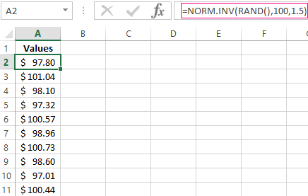
The prime cost of the X product is $100. The entire batch is subject to a standard distribution. The random variable also obeys a standard probability distribution.
Under such conditions, the average value of the range is $100. Let’s generate an array and build a chart that obeys a standard distribution with a standard deviation of $1.5.
Use the function:
Excel calculates the values in the range of probabilities. As the probability of manufacturing a product with a prime cost of $100 is maximal, the formula returns values that are close to 100 more often than other values.
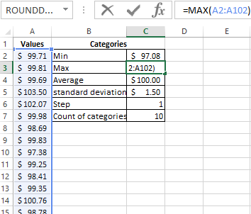
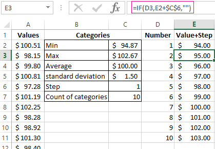
Let’s proceed to building the chart. First of all, you need to create a table containing the categories. To do this, split the array into periods:
- Determine the minimum and maximum values in the range using the =MIN(A2:102) and =MAX(A2:102) functions.
- Indicate the value of each period or step. In our example, it’s equal to 1.
- The number of categories is 10.
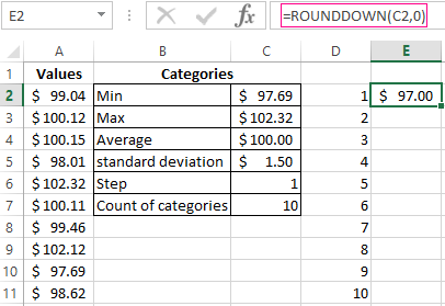
- The lower limit of the table containing the categories is the nearest multiple number rounded down. Enter the formula =ROUNDDOWN(C2,0) into the E1 cell.
- In the E2 cell and below, the formula will look as follows:
That is, each subsequent value is increased by the specified step size.
- Let’s calculate the number of variables in the given interval. Use the function:
The formula will look as follows:
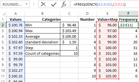
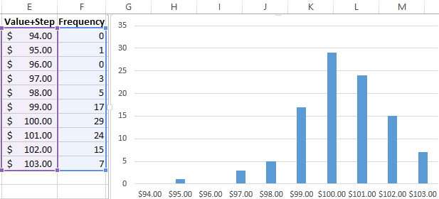
Based on the obtained data, we can build a chart with a normal distribution. The value axis represents the number of variables in the interval; the category axis represents the periods.
A chart with a normal distribution is built. As it should be, its shape resembles a bell.
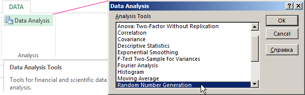
There’s a much simpler way to do the same with the help of the «Data Analysis» package. Select «Random Number Generation».
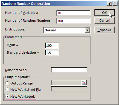
Click here to learn how to set up the standard feature: «Data Analysis».
Fill in the generation parameters. Set the distribution as «Normal».
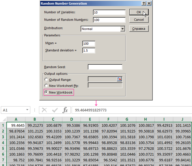
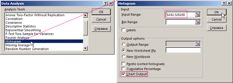
Click OK. It gives us a set of random numbers. Open the «Data Analysis» once again. Select «Histogram». Configure the parameters. Be sure to check the «Chart Output» box.
The obtained result is as follows:
Download random number generators in Excel
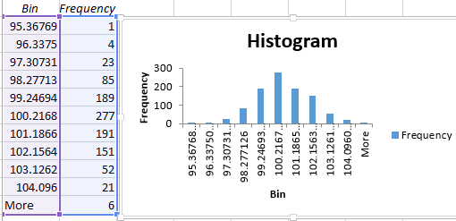
An Excel chart with a standard distribution has been built.
There may be cases when you need to generate random numbers in Excel.
For example, to select random winners from a list or to get a random list of numbers for data analysis or to create random groups of students in class.
In this tutorial, you will learn how to generate random numbers in Excel (with and without repetitions).
Generate Random Numbers in Excel
There are two worksheet functions that are meant to generate random numbers in Excel: RAND and RANDBETWEEN.
- RANDBETWEEN function would give you the random numbers, but there is a high possibility of repeats in the result.
- RAND function is more likely to give you a result without repetitions. However, it only gives random numbers between 0 and 1. It can be used with RANK to generate unique random numbers in Excel (as shown later in this tutorial).
Generate Random Numbers using RANDBETWEEN function in Excel
Excel RANDBETWEEN function generates a set of integer random numbers between the two specified numbers.
RANDBETWEEN function takes two arguments – the Bottom value and the top value. It will give you an integer number between the two specified numbers only.
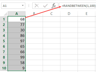
For example, suppose I want to generate 10 random numbers between 1 and 100.
Here are the steps to generate random numbers using RANDBETWEEN:
- Select the cell in which you want to get the random numbers.
- In the active cell, enter =RANDBETWEEN(1,100).
- Hold the Control key and Press Enter.
This will instantly give me 10 random numbers in the selected cells.
While RANDBETWEEN makes it easy to get integers between the specified numbers, there is a high chance of repetition in the result.
For example, when I use the RANDBETWEEN function to get 10 random numbers and use the formula =RANDBETWEEN(1,10), it gives me a couple of duplicates.
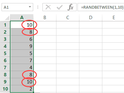
If you’re OK with duplicates, RANDBETWEEN is the easiest way to generate random numbers in Excel.
Note that RANDBETWEEN is a volatile function and recalculates every time there is a change in the worksheet. To avoid getting the random numbers recalculate, again and again, convert the result of the formula to values.
Generate Unique Random Numbers using RAND and RANK function in Excel
I tested the RAND function multiple times and didn’t find duplicate values. But as a caution, I recommend you check for duplicate values when you use this function.
Suppose I want to generate 10 random numbers in Excel (without repeats).
Here are the steps to generate random numbers in Excel without repetition:
Now you can use the values in column B as the random numbers.
Note: RAND is a volatile formula and would recalculate every time there is any change in the worksheet. Make sure you have converted all the RAND function results to values.
Caution: While I checked and didn’t find repetitions in the result of the RAND function, I still recommend you check once you have generated these numbers. You can use Conditional Formatting to highlight duplicates or use the Remove Duplicate option to get rid of it.
You May Also Like the Following Excel Tutorials:
- Automatically Sort Data in Alphabetical Order using Formula.
- Random Group Generator Template
- How to Shuffle a List of Items/Names in Excel?
- How to Do Factorial (!) in Excel (FACT function)
What Are Random Numbers In Excel?
Random numbers in Excel are used when we want to randomize our data for a sample evaluation. These numbers generated randomly. There are two built-in functions in Excel which give us random values in cells, RAND and RANDBETWEEN functions.
RAND() function provides us with any value from the range 0 to 1, whereas =RANDBETWEEN() takes input from the user for an arbitrary number range.
Randomness has many uses in science, art, statistics, cryptography, and other fields.
Generating Random numbers in excel is important because many things in real life are so complicated that they appear random. Therefore, to simulate those processes, we need random numbers.
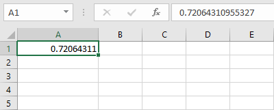
For instance, we can generate a random number in excel using =RAND().
- Step 1: Insert the =RAND() in cell A1.

- Step 2: Press Enter.

Likewise, we can generate random numbers using random numbers in excel.
Table of contents
- What Are Random Numbers In Excel?
- How To Generate Random Numbers In Excel?
- How To Generate Random Numbers In Excel For More Than One Cell?
- RANDBETWEEN() Function
- Important Things To Remember
- Random Numbers In Excel – Project 1
- Random Numbers In Excel – Project 2 – Head And Tail
- Random Numbers In Excel – Project 3 – Region Allocation
- Random Numbers In Excel – Project 4 – Creating Ludo Dice
- Frequently Asked Questions (FAQs)
- Recommended Articles
- Random Numbers in excel is used to generate numbers in excel.
- The Random numbers in Excel function help in generating random data for sample evaluation.
- Remember, the Random Numbers in excel is a worksheet function (WS function)
- Excel has two built-in Random functions which yield random values. They are =RAND() function and =RANDBETWEEN().
- The =RAND() provides us with any value from the range 0 to 1, whereas the =RANDBETWEEN() function takes input from the user for an arbitrary number range.

You are free to use this image on your website, templates, etc, Please provide us with an attribution linkArticle Link to be Hyperlinked
For eg:
Source: Random Numbers in Excel (wallstreetmojo.com)
How To Generate Random Numbers In Excel?
There are several methods to generate a random number in Excel. We will discuss the two of them: RAND() and RANDBETWEEN() functions.
You can download this Generate Random Number Excel Template here – Generate Random Number Excel Template
#1 – RAND() Function
To generate a random number in Excel between 0 and 1(excluding), we have a RAND() function in Excel.
RAND() functions return a random decimal number that is equal to or greater than 0 but less than 1 (0 ≤ random number <1). In addition, the RAND function recalculates when a worksheet is opened or changed (volatile function).
The RAND function returns the value between 0 and 1 (excluding).
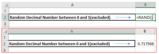
We must type =RAND() in the cell and press Enter. The value will change whenever any change is made in the sheet.
How To Generate Random Numbers In Excel For More Than One Cell?
If we want to generate random numbers in Excel for more than one cell, then we need:
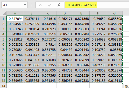
- First, select the required range, type =RAND(), and press Ctrl+Enter to give us the values.
How to Stop Recalculation of Random Numbers in Excel?
As the RAND function recalculates, if any change in the sheet is made, we must copy and then paste the formulas as values if we do not want values to be changed every time. For this, we need to paste the values of the RAND() function using Paste Special so that it would no longer be a result of the “RAND ()” function. It will not be recalculated.
To do this,
- We need to make the selection of the values.
- Press the Ctrl+C keys to copy the values.

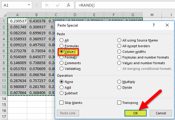
- Without changing the selection, press the Alt+Ctrl+V keys to open the Paste Special dialog box.
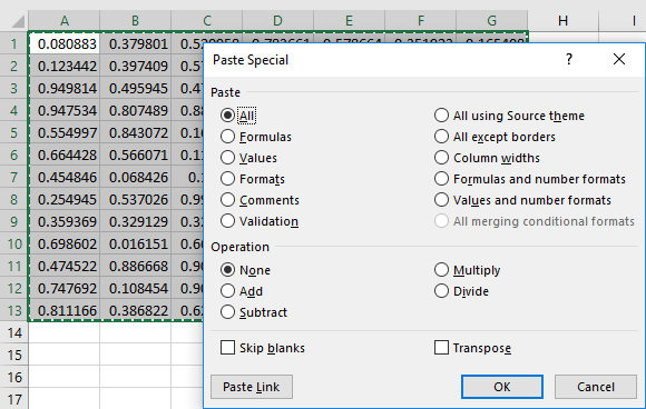
- Choose Values from the options and click on OK.
We can see that the value in the formula bar is the value itself, not the RAND() function. Now, these are only values.
There is one more way to get the value, only not the function as a result, but that is only for one cell. If we want the value the very first time, not the function, then the steps are:
- First, type =RAND() in the formula bar, press F9, and press the Enter key.
After pressing F9, we get the value only.
Value From A Different Range Other Than 0 And 1 Using RAND()
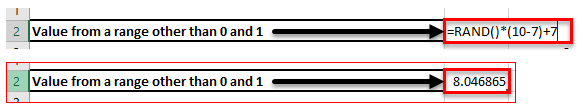
As the RAND function returns a random decimal number between 0 and 1 only, if we want the value from a different range, then we can use the following function:
Let ‘a’ be the start point.
And ‘b’ be the end point
The function would be ‘RAND()*(b-a)+a’
For example, if we have 7 as “a” and 10 as “b,” then the formula would be “=RAND()*(10-7)+7.”
RANDBETWEEN() Function
As the function’s name indicates, this function returns a random integer between given integers. Like the RAND() function, this function also recalculates when a workbook is changed or opened (volatile function).
The formula of the RANDBETWEEN Function is:
- Bottom: An integer representing the lower value of the range.
- Top: An integer representing the lower value of the range.
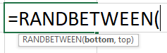
To generate random numbers in Excel for the students between 0 and 100, we will use the RANDBETWEEN function.
First, we must select the data, type the formula, =RANDBETWEEN(0,100), and press the Ctrl + Enter keys. You can prefer the below-given screenshot.
As values will recalculate, we can only use Alt+Ctrl+V to open the Paste Special dialog box to paste as values.
Follow the steps given below in the screenshot.
Like the RAND() function, we can also type the RANDBETWEEN function in the formula bar, pressing F9 to convert the result into value, and then press the Enter key.
Important Things To Remember
- If the bottom is greater than the top, the RANDBETWEEN function will return #NUM! Error.
- If either of the supplied arguments is non-numeric, the function will return #VALUE! Error.
- Both RAND() and RANDBETWEEN() functions are volatile functions (recalculates). Hence, it increases the processing time and can slow down the workbook.
Random Numbers In Excel – Project 1
We can use the RANDBETWEEN() function for getting random dates between two dates.
We will be using two dates as the bottom and top arguments.

After making the selection, we need to copy down the formula using the shortcut (Ctrl+D).

We can change the start date (D1) and end date (E1) to change the top and bottom values for the function.
Random Numbers In Excel – Project 2 – Head And Tail
To randomly choose head and tail, we can use the CHOOSE function in excel with the RANDBETWEEN function.

We need to copy the formula into the next and next cell every time in the game, and Head and Tail will come randomly.
Random Numbers In Excel – Project 3 – Region Allocation
Many times, we have to imagine and create data for various examples. For example, suppose we have data for sales, and we need to allocate three different regions to every sale transaction.
Then, we can use the RANDBETWEEN function with the CHOOSE function.

We can drag the same for the remaining cells.
Random Numbers In Excel – Project 4 – Creating Ludo Dice
Using the RANDBETWEEN function, we can also create dice for Ludo. We need to use the RANDBETWEEN function in Excel VBA for the same. Please follow the below steps:
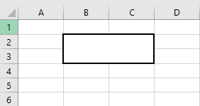
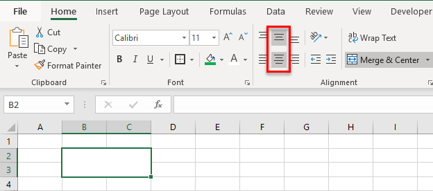
- Merge the four cells (B2:C3) using Home Tab → Alignment Group → Merge & Center.
- Apply the border to the merged cell using the shortcut key (ALT+H+B+T) by pressing one key after another.
- Center and middle align the value using Home Tab → Alignment Group → Center and Middle Align commands.
- To create the button, use Developer tab → Controls Group → Insert → Command Button
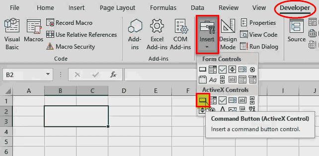
- Create the button and choose View Code from the Controls group on Developer.

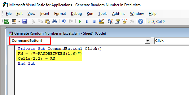
- After choosing CommandButton1 from the dropdown, paste the following code:
RN = (“=RANDBETWEEN(1,6)”)
Cells(2, 2) = RN
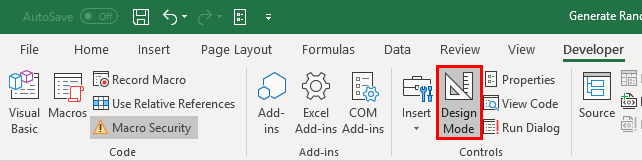
Please save the file using the .xlsm extension as we have used the VBA code in the workbook. After coming to the Excel window, deactivate the Design Mode.
Now, whenever we click the button, we get a random value between 1 and 6.
Frequently Asked Questions (FAQs)
1. What is Random Numbers in excel?
Random Numbers in excel is a built-in function used to generate random values. It is used when we have to calculate sample evaluation for random values.
2. What are the two functions used to generate random numbers in excel?
In excel, we can generate numbers using two functions. They are: =RAND() and =RANDBETWEEN().
The =RAND() provides us with any value from the range 0 to 1, whereas the =RANDBETWEEN() function takes input from the user for an arbitrary number range.
3. How to use RAND function in excel?
RAND() generates random numbers between 0 to 1.
For example, consider the below image where we have inserted the RAND() in a blank cell.

As soon as we press Enter¸ we can see that the function has generated a random number below 1 as shown in the below image.

Similarly, we can generate random numbers between 0 to 1, using random numbers in excel function.
Recommended Articles
This article is a guide to Random Numbers in Excel. Here, we discuss generating random numbers in Excel using the RAND() and RANDBETWEEN functions along with multiple projects and downloadable Excel templates. You may also look at these useful functions in Excel: –
- Randomize List in Excel
- Auto Number in Excel
- VBA Random Number
- RAND Function in Excel
Excel allows us to get a random value from a list or table, by using the INDEX, RANDBETWEEN and ROWS functions. This step by step tutorial will assist all levels of Excel users in understanding how to get a random value from the list using these 3 functions.
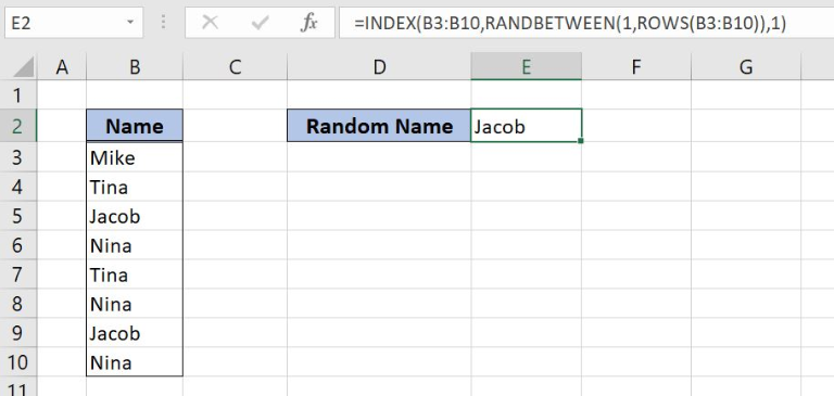 Figure 1. The final result of the functions
Syntax of the INDEX formula
=INDEX(array, row_num, [column_num])
The parameters of the INDEX function are:
- array – a list of values where we want to find a value from a certain position
- row_num – a row from which we want to get a value
- [column_num] – a column from which we want to get a value. It’s a non-mandatory parameter and if it’s omitted it’s by default 1.
Syntax of the RANDBETWEEN formula
=RANDBETWEEN(bottom, top)
The parameters of the RANDBETWEEN function are:
- bottom – a value from which we want to get a random value
- top – a value to which we want to get a random value
Syntax of the ROWS formula
=ROWS(array)
The parameter of the ROW function is:
- array – an array for which we want to get the total number of rows.
Setting up Our Data for the Functions
In column B (“Names”), we have the list of names for which we want to find the random name. The result will be stored in the cell E3
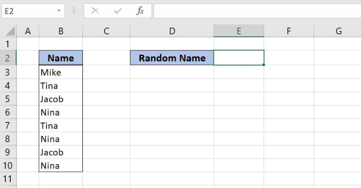 Figure 2. Data that we will use in the example
Get a Random Name from the List of Names
In the cell E3, we want to get the random name from the list of names in the range B3:B10.
The formula looks like:
=INDEX(B3:B10, RANDBETWEEN(1, ROWS(B3:B10)), 1)
The array is B3:B10. The row_num is RANDBETWEEN(1, ROWS(B3:B10)), while the column_num is 1.
To apply the formula, we need to follow these steps:
- Select cell E3 and click on it
- Insert the formula:
=INDEX(B3:B10, RANDBETWEEN(1, ROWS(B3:B10)), 1) - Press enter.
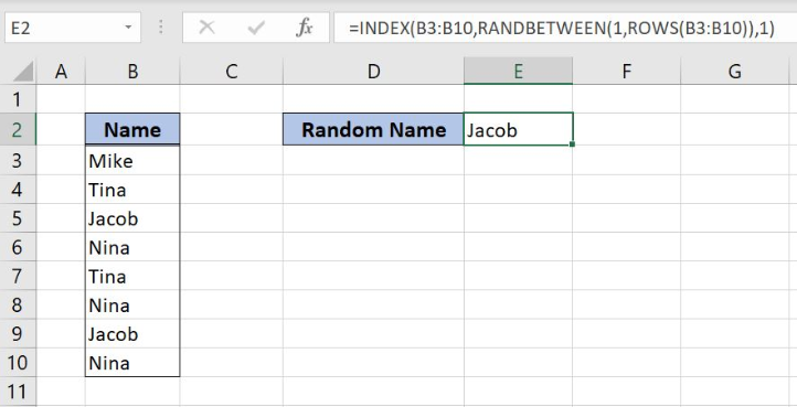 Figure 3. Using the INDEX function to get a random name from the list
The INDEX function searches the B3:B10 range. The row_num is the result of the RANDBETWEEN function, which returns a random number between 1 and 8. In this example, this function returned 3, so the INDEX returns the value from the third row. Therefore, the result of the formula in the cell E3 is “Jacob”.
Most of the time, the problem you will need to solve will be more complex than a simple application of a formula or function. If you want to save hours of research and frustration, try our live Excelchat service! Our Excel Experts are available 24/7 to answer any Excel question you may have. We guarantee a connection within 30 seconds and a customized solution within 20 minutes.
Sometimes, you want to create random values in Excel. For example, when you want to simulate some kind of statistical distribution, make up random key codes or want to pre-fill some database. In this article, we’ll take a look at the two Excel formulas RAND and RANDBETWEEN with a lot of examples.
How to create random values in general
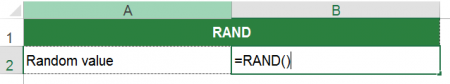
There is a simple formula to generate random numbers: RAND. If you type =RAND() into a cell, you’ll get a number between 0 and 1.
Two comments:
- The RAND formula has no argument. So don’t type anything between the brackets.
- You’ll get many decimals. We’ll explore later on how to use that.
That’s the easy case – let’s take it a step further.
Create random values with decimals and between a minimum and maximum value
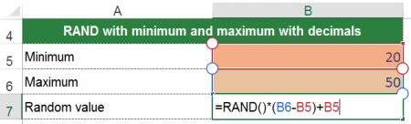
What do you do, if you want to have random number between 20 and 50 for example?
Use the RAND formula and do some maths: The interval is 30 (=50-20). We have to multiply =RAND() by 30. That means, the random number will be between 0 and 30. Now we only have to add 20. The result is then always between 20 and 50. If you want to create whole numbers, please add the ROUND formula.
In more mathematical terms: If you want to get a random number between a and b, you have to type
=RAND()*(b-a)+a
Create random values without decimals (whole numbers) with a minimum and maximum value
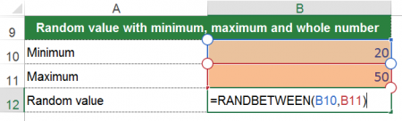
If you want to get whole number you got two options: Either you use the method from our example before and wrap it into the ROUND formula with 0 decimals. Or you use the more elegant soluation: Use the RANDBETWEEN formula.
RANDBETWEEN works similar to RAND but has two arguments: the bottom (in our case 20) and the top value (in our example 50). The complete formula looks like this: =RANDBETWEEN(20,50) .
As said before: Please note that RANDBETWEEN only returns integer values. So if you some more decimals you should go with the first option.
Do you want to boost your productivity in Excel?
Get the Professor Excel ribbon!

Add more than 120 great features to Excel!
Create even numbers with a minimum and maximum value
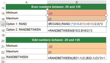
Let’s take a look at a special example. This example should provide an idea of how to solve more complicated cases. The example: You want to get an even number between -20 and +20.
Let’s set up the formula step by step using the RAND formula:
- First you want to get a decimal number between the range 0 and 40 (that equals the distance between -20 and +20):
=RAND()*40 - Next you move the range from “0 to 40” to “-20 to 20” by subtracting 20:
=RAND()*40-20 - Now you already got a random number with decimals between -20 and +20. As the next step, you have to make it an even number. Therefore, you divide it by 2 and round it to 0 decimals. That way, you got a whole number between -10 and +10. Now you only multiply it by 2 . That’s it.
=ROUND((RAND()*40-20)/2,0)*2
There is also a slightly shorter way using RANDBETWEEN:
=RANDBETWEEN(-20/2,20/2)*2One more note: If you want to get odd number, just add 1 in the end (and change the minimum and maximum values accordingly). So if you want to get an odd value between -20 and +20:
=RANDBETWEEN((B21-1)/2,(B22-1)/2)*2+1Create normal distributed values
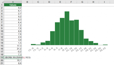
The RAND and RANDBETWEEN produce even distributed values. That means, each value between your minimum and maximum will come up with the same probability. Sometimes you don’t want that. Instead you want to get values with a distribution, let’s say the most popular normal distribution.
In such case you can combine the RAND formula with the NORM.INV formula. That way, you can create random values with a underlying normal distribution.
You need to specify:
- The probability (with the RAND() formula).
- The mean. This determines where the maximum is located.
- The standard deviation determines the width of the data.
If you put these input values together (let’s say with the mean of 10 and the standard deviation of 5), the formula looks like this:
=NORM.INV(RAND(),10,5)Create random small and capital letters
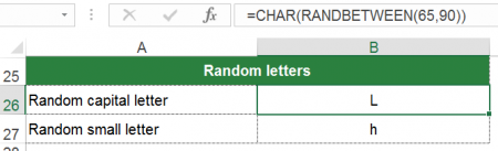
You can also create random letters. Therefore you have to use a so-called ASCII code: Every character has a number (not only in Excel). Here is a list of ASCII codes. You only have to wrap CHAR formula around the RANDBETWEEN formula (with the correct minimum and maximum values). That way, Excel translates your random number into the corresponding character.
The formula for capital letters (they occupy numbers 65 to 90 among the ASCII codes):
=CHAR(RANDBETWEEN(65,90))The formula for small letters:
=CHAR(RANDBETWEEN(97,122))Final notes and download
Some more comments on both formulas (RAND and RANDBETWEEN):
- Both formulas are volatile. That means that every time when you recalculate your workbook, the random value will change.
- Please note: RAND and RANDBETWEEN create even distributed numbers by default.
- Please feel free to download all the examples above from this direct download link.
Has this article helped you? Why don’t you subscribe to our free Excel newsletter?