
Excel for Microsoft 365 Excel for Microsoft 365 for Mac Excel for the web Excel 2021 Excel 2021 for Mac Excel 2019 Excel 2019 for Mac Excel 2016 Excel 2016 for Mac Excel 2013 Excel 2010 Excel 2007 Excel for Mac 2011 Excel Starter 2010 More…Less
This article describes the formula syntax and usage of the RAND function in Microsoft Excel.
Description
RAND returns an evenly distributed random real number greater than or equal to 0 and less than 1. A new random real number is returned every time the worksheet is calculated.
Syntax
RAND()
The RAND function syntax has no arguments.
Remarks
-
To generate a random real number between a and b, use:
=RAND()*(b-a)+a
-
If you want to use RAND to generate a random number but don’t want the numbers to change every time the cell is calculated, you can enter =RAND() in the formula bar, and then press F9 to change the formula to a random number. The formula will calculate and leave you with just a value.
Example
Copy the example data in the following table, and paste it in cell A1 of a new Excel worksheet. For formulas to show results, select them, press F2, and then press Enter. You can adjust the column widths to see all the data, if needed.
|
Formula |
Description |
Result |
|---|---|---|
|
=RAND() |
A random number greater than or equal to 0 and less than 1 |
varies |
|
=RAND()*100 |
A random number greater than or equal to 0 and less than 100 |
varies |
|
=INT(RAND()*100) |
A random whole number greater than or equal to 0 and less than 100 |
varies |
|
Note: When a worksheet is recalculated by entering a formula or data in a different cell, or by manually recalculating (press F9), a new random number is generated for any formula that uses the RAND function. |
Need more help?
You can always ask an expert in the Excel Tech Community or get support in the Answers community.
See Also
Mersenne Twister algorithm
RANDBETWEEN function
Need more help?
RAND and RANDBETWEEN have the same function — to generate random numbers. The result of the RAND function is a uniformly distributed random number (real), by default the range of such numbers is from 0 to 1. How Do Functions Work?
Random number generators RAND and RANDBETWEEN in Excel
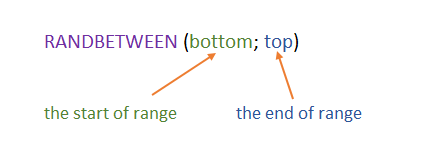
The syntax of such a function does not take any arguments. That is, it is not necessary to write anything inside the brackets, as we are already used to when working in Excel. RANDBETWEEN has the following syntax:
Let’s start with the simplest first example, which will take up only one cell. In cell A1 we write the RAND function, we have no arguments in brackets and press Enter:
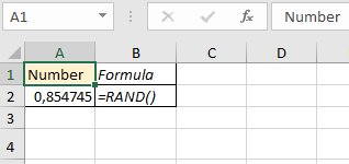
We got a random number in the range from 0 to 1. Now let’s copy the formula down a few cells and see some feature in the work of RAND:
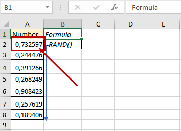
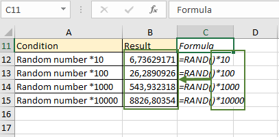
Note that the values in the first cell has changed. When we copied the function, the numbers were recalculated and new values were determined that correspond from 0 to 1. In the next example, we will look at how you can influence the returned result. Let’s create a table in which we will determine some conditions. We can increment the return value. For instance, to get a number greater than 1, we add a multiplication by 10 to the RAND function:
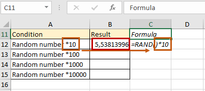
And so we change the value of the number as much as necessary. If you need two characters before the coma, multiply by 100 and so on. The same principle can be applied to the decimal fraction RANDBETWEEN function. Let’s fill in our column:
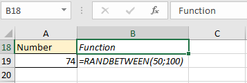
If you need to limit the minimum and maximum value among a set of random numbers, then you need to use RANDBETWEEN. By setting the range limits, we get the generated numbers that do not go beyond the range:
In the example, we specified the boundaries of the range as arguments. Now, the result corresponding to the conditions was returned. Copy the formula down to several cells:
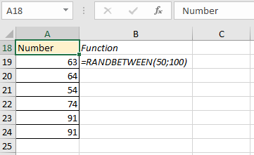
As you can see, all values are within the specified frames.
How to use RAND and RANDBETWEEN in practice?
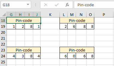
Where can such a simple and easy, seemingly incapable of significant calculations function be required? For example, when generating a PIN code. We have 4 cells, the boundaries for the RANDBETWEEN function will be 0 and 9. In cell G19, we write the formula and copy it in order:
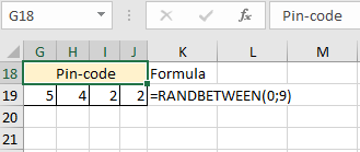
We have formed a 4-digit PIN code. But what if you need to get multiple random values for a PIN? Then you need to start recalculation. You can do this manually by pressing F9 on your keyboard. Now we have 4 fields with PIN codes with certain values:
Press F9 and see what result we have now:
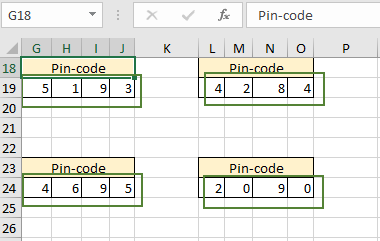
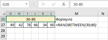
In all fields, in all cells, the values changed randomly. This can be done as many times as needed. Random number generation can also be used in different lotteries. For example, we have a range from 30 to 80, and we need to get 6 any numbers from this set. It is just as easy to complete this task — we specify “30” as the first argument for the function RANDBETWEEN, “80” as the second argument and copy for the next 5 cells:
We can also conclude that all tasks using the RANDBETWEEN function return a set of exclusively integer numbers. But how to solve the problem when you need results that are greater than 1, and a fractional remainder. We know that the RAND function partially fulfills this condition, since it returns the contents of the range from 0 to 1 with a fraction. And the RANDBETWEEN function fulfills the second of two conditions — you can specify the desired array. It turns out that you need to combine these two functions so that their joint calculation returns the desired result:

But now there is a small flaw in the formula. Let’s recalculate the formula and take a closer look at the new values:
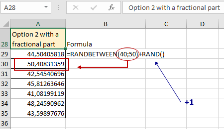
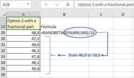
Now we can observe that we have a value that goes beyond the upper bound of the array. This is because RAND works according to the simple logic of mathematics and simply performs the specified addition operation — adding the generated fractional part to the upper bound. In order to avoid this disadvantage, you need to use a simple rule of mathematics. If you need fractional values from 40 to 50, then in the arguments for RANDBETWEEN we indicate the boundaries of 400 and 500 and divide the function by 10. Now we will return results from 40.0 to 50.0:
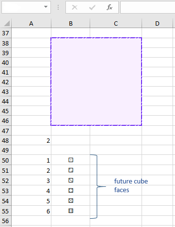
Having mastered the functions of generating random numbers, let’s try to create a functional dice that can be used like a real one. Let’s start by selecting and merging cells B38:C46. This will be our face of the cube. If you wish, you can add decorative effects, for example, make an unusual color frame and fill, preferably using a light background:
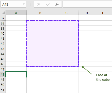
The address of this cell will be B38, because in the case of merging several cells, its address will be the upper leftmost cell before the merging. Later we will return to the square, but for now, we need to implement the main work of the die — «throw» the numbers from 1 to 6 in random order. In cell A48, start writing the formula:
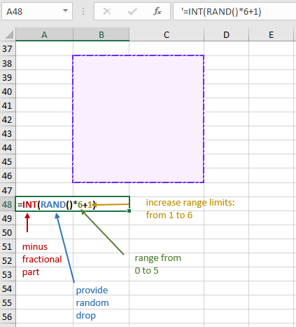
The way this formula works is as follows:
- RAND will still generate numbers from 0 to 1 with a fraction.
- The multiplication operation will change our range — it will turn out from 0.0 to 5.0.
- We don’t need a fraction, so we use an INT, in which we put a RAND with multiplication and addition. At this stage, we will get the range (0;5).
- Add a unit to get the boundaries (1;6).
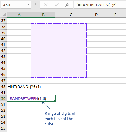
The same range can be obtained through RANDBETWEEN by simply specifying the desired boundaries:
We leave in cell A48 the option that we like best. To make the cube really look like a real one, we use the images of its faces, which we will add later to a large square. Cells A50:A55 will be filled with numbers from 1 to 6. Opposite the corresponding number, using Unicode characters, we will copy characters from the unicode-table.com resource to display all 6 faces:
Now we need to make sure that the “throw” of the die is displayed directly in cell B38. For this we created this large array. It is necessary to associate a randomly generated value from the RANDBETWEEN formula with the images of the face of the cube and the large cell B38. You can do this in several ways. The first is using the IF function. Since this formula has only two arguments, and we need to display 6 variations, we use the IF nesting property. In cell B38, enter the formula:
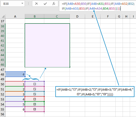
The principle of operation is simple: the first condition is checked and either cell B50 (value_if_true) is returned, or the transition to the “value_if_false” argument, which consists of a new IF with arguments and values. And so on the chain. Note that we don’t use the sixth IF at the end, but just specify value_if_false for the fifth «IF» because that’s the end of the chain and the sixth IF is not necessary. It is possible to use Unicode characters in the nested IF, which are represented by face images, instead of input addresses with face icons. There is another option for displaying the corresponding face. In cell C50, write the formula IF(A50=F$48;B50) and copy it up to cell C55 (the dollar symbol will ensure copying without unnecessary cell shifts). The formula checks if cell A50 contains the value from cell A48, then returns either a dice icon or empty text. After that, you need to provide a link between column C50:C55 and cube B38. To do this, you can use two options: either chain cells together using an ampersand, or through CONCATENATE, which performs the same option:
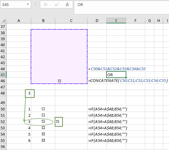
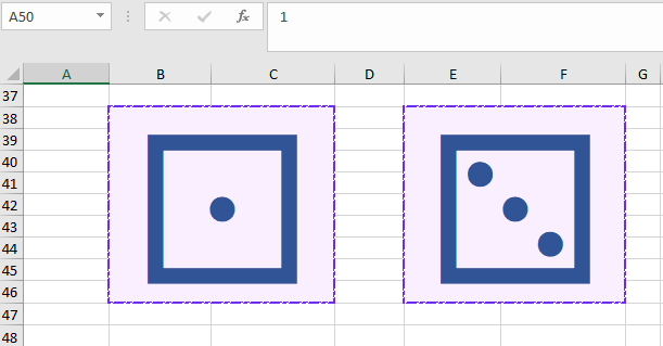
Both formulas from cells D44 and D46 work the same way: the concatenation of cells displays the text contained in them together, but since among these cells only one will always display a cube icon, and the other five will display empty text, the only unique one will be displayed in a large square icon. Now our cube is not looks exactly like the real one. In order to improve the graphic image, let’s increase the text font of the cube in our case by 180. We can also change the color of the cube at will. If the game needs a pair of dice, just copy the entire array with the big square and the calculation array below, and place it next to the first one. Now we have two beautiful and functional dice. We can also continue to improve and hide all the calculations that are under the dice:
- Select the entire range below the cubes.
- On the «Home» tab, open a window in the «Number» subgroup.
- Among the categories, select «all formats» and in the «Type» enter ;;; (three times dot with quotation mark).
- Click «ok» and observe the final result:
 Download examples of use RANDBETWEEN and RAND functions in Excel
In the cell A40 in the formula field, we still see that the text has not been removed but is hidden from view. To start a new «throw», it is enough to start the recalculation of functions — press the F9.
Бывают случаи, когда мы хотим смоделировать случайность, фактически не выполняя случайный процесс. Например, предположим, что мы хотим проанализировать конкретный случай 1000000 подбрасываний честной монеты. Мы могли бы подбросить монету миллион раз и записать результаты, но это займет некоторое время. Одна альтернатива – использовать функции случайных чисел в Microsoft Excel. Обе функции RAND и RANDBETWEEN предоставляют способы моделирования случайного поведения.
Содержание
- Функция RAND
- Функция RANDBETWEEN
- Предостережения при пересчете
- Действительно случайно
Функция RAND
Мы начнем с рассмотрения RAND функция. Эта функция используется путем ввода в ячейку Excel следующего текста:
= RAND ()
Функция не принимает аргументов в круглых скобках. Она возвращает случайное действительное число от 0 до 1. Здесь этот интервал действительных чисел считается единым пространством выборки, поэтому при использовании этой функции с равной вероятностью будет возвращено любое число от 0 до 1.
Функцию RAND можно использовать для моделирования случайного процесса. Например, если мы хотим использовать это для имитации подбрасывания монеты, нам нужно будет использовать только функцию ЕСЛИ. Когда наше случайное число меньше 0,5, тогда функция может возвращать H для голов. Когда число больше или равно 0,5, тогда мы могли бы заставить функцию возвращать T для хвостов.
Функция RANDBETWEEN
Вторая функция Excel, работающая со случайностью, называется СЛУЧАЙНОМЕР. Эта функция используется путем ввода следующего текста в пустую ячейку Excel.
= RANDBETWEEN ([нижняя граница], [верхняя граница])
Здесь текст в квадратных скобках должен быть заменен двумя разными числами. Функция вернет целое число, которое было случайно выбрано между двумя аргументами функции. Опять же, предполагается единообразное пространство выборки, что означает, что каждое целое число с равной вероятностью будет выбрано.
Например, оценка RANDBETWEEN (1,3) пять раз может привести к 2, 1, 3, 3, 3.
Этот пример показывает важное использование слова «между» в Excel. Это следует интерпретировать в широком смысле, включая верхнюю и нижнюю границы (при условии, что они являются целыми числами).
Опять же, с использованием функции ЕСЛИ мы могли бы очень легко смоделировать подбрасывание любого количества монет. Все, что нам нужно сделать, это использовать функцию RANDBETWEEN (1, 2) вниз по столбцу ячеек. В другом столбце мы могли бы использовать функцию ЕСЛИ, которая возвращает H, если из нашей функции RANDBETWEEN была возвращена 1, и T в противном случае.
Конечно, есть и другие возможности использования функции СЛУЧАЙНА. Это было бы простое приложение для моделирования качения матрицы. Здесь нам понадобится RANDBETWEEN (1, 6). Каждое число от 1 до 6 включительно представляет одну из шести сторон игральной кости..
Предостережения при пересчете
Эти функции, работающие со случайностью, будут возвращать разные значения при каждом пересчете. Это означает, что каждый раз, когда функция оценивается в другой ячейке, случайные числа будут заменяться обновленными случайными числами. По этой причине, если конкретный набор случайных чисел будет изучен позже, было бы целесообразно скопировать эти значения, а затем вставить эти значения в другую часть рабочего листа.
Действительно случайно
Мы должны быть осторожны при использовании этих функций, потому что они являются черными ящиками. Нам неизвестен процесс, который Excel использует для генерации случайных чисел. По этой причине трудно точно знать, что мы получаем случайные числа.
Not every user will have a need for random numbers in Excel. Most people work with fixed numbers and formulas and may have no need for random numbers to appear in their reports.
However, a random number generator does have a huge use when working with different scenarios on a set of data or when performing various statistical analyses.
A financial model may use a stochastic simulation that is dependent on probabilities. The model may need to be run thousands of times, but with the random number generator providing the parameters of each simulation.
Whatever your need for random numbers, Excel has several ways to generate them.
In this post, I’ll show you all the methods you can use to insert random numbers into your workbooks.
Generate Random Numbers with the RAND function
The first way I will show you is the easiest way to generate random values in Excel.
There is a very simple RAND function that requires no parameters and will generate a random number between 0 and 1.
Syntax for the RAND Function
= RAND ( )This function has no required or optional arguments. The function is always entered with an empty set of parenthesis.
This function will generate a decimal random number between 0 and 1, but not including 0 or 1.
Repeated values are possible but unlikely since the RAND function produces numbers from a continuous range of numbers.
The values that are returned will follow a uniform distribution. This means that any number between 0 and 1 is equally likely to be returned.
Generate Random Numbers Between Any Two Numbers
A decimal number between 0 and 1 may not be too useful if you need numbers between 1 and 10.
But you can use a simple formula involving the RAND function to generate random numbers between any two numbers.
= RAND ( ) * ( Y - X ) + XIn general, you can create a random number between X and Y by using the above formula.
= RAND ( ) * 9 + 1For example, to generate numbers between 1 and 10 you can use the above formula.
This multiplies the random number generated by 9 and then adds 1 to it. This will produce decimal numbers between 1 and 10.
Generate Random Integer Numbers Between Any Two Numbers
Another possible need you may encounter is to generate random whole numbers between two given numbers. This can also be done using a simple formula.
= ROUND ( RAND ( ) * ( Y - X ) + X, 0 )In general, you can use the above formula to generate random integer numbers between two values X and Y.
= ROUND ( RAND ( ) * 9 + 1, 0 )For example, the above formula will create random integer numbers between 1 and 10.
This is the same formula as before, but using the ROUND function to round to zero decimal places.
You can copy this formula down the column on the spreadsheet, and if you keep pressing F9 to re-calculate, you will see various combinations of numbers from 1 to 10.
Since the set of possible numbers is discrete, the random numbers generated may well be duplicated in the list, depending on what the minimum and maximum are of the range.
= ROUND ( RAND ( ) * ( 4 - -3 ) + -3, 0 )This also works for producing negative numbers. Suppose you need to generate random integer numbers between -3 and 4, then the above formula will be what you need.
Multiplying the RAND function by 7 will produce random numbers between 0 and 7. Add -3 to the result and round to zero decimal places, and this will give the range of random numbers of -3 to 4.
Generate Random Numbers using the RANDBETWEEN Function
Excel has a useful function for generating random numbers within a range of an upper and lower number.
This is easier to use than using the RAND function as it includes extra operators to arrive at your specific range.
Syntax for the RANDBETWEEN Function
= RANDBETWEEN ( bottom, top )- bottom is the lower range for the values to return.
- top is the upper range for the values to return.
Both of these arguments are required.
This function will produce random integer numbers between the bottom and top values. This function will also return the upper and lower limits as possible values as it’s not strictly between in this function.
Example with the RANDBETWEEN Function
= RANDBETWEEN ( -3, 4 )For example, if you wanted random numbers between -3 and 4, as in the previous example, you can use the above formula.
Note that the RANDBETWEEN function can only produce integer numbers. There is no way of making the function produce decimal numbers. However, it is considerably less complicated than using the RAND function with operators to achieve the same result.
Generate Random Numbers with the RANDARRAY Function
Usually, it’s the case that you don’t want just a single random value but an entire set of random values.
The RANDARRAY function is the perfect solution for this.
It will populate a range of cells with an array of random numbers, which can be very powerful.
This function is only available on the Microsoft 365 version of Excel.
Syntax for the RANDARRAY Function
= RANDARRAY ( [rows], [columns], [min], [max], [whole_number] )- Rows is the number of rows to return.
- Columns is the number of columns to return.
- Min is the minimum value for the random numbers.
- Max is the maximum value for the random numbers.
- Whole_Number is TRUE to return whole numbers, and FALSE to return decimal numbers.
All the arguments are optional for this function.
If no parameters are included, you will get a single random number with decimal places, in the same way as the RAND function.
Example with the RANDARRAY Function
= RANDARRAY ( 4, 3, 6, 14, TRUE )To generate an array of 4 rows and 3 columns of whole random numbers between 6 and 14 you can use the above formula.
This will produce an array of values. Notice the blue border around the numbers? These are all produced from a single formula!
Note that the top left-hand corner of the array is always anchored on the cell that the formula is in. Pressing F9 to recalculate the spreadsheet will change all the numbers in the array.
If you do not put a minimum or maximum value, the default of 0 to 1 will be used.
The minimum value must be less than the maximum value otherwise there will be a #VALUE! error.
The array will automatically resize if you change either the rows or columns parameters in the RANDARRAY formula. This is why they’re known as dynamic arrays.
Warning: If there is already data in one of the cells in the output range that you have entered, you will get a #SPILL! error. No data will be overwritten.
Generate Random Numbers with the Analysis Tools Add-In
There is another method that can be used to insert random numbers without using a formula.
You can use an add-in to create random numbers. Excel comes with an Analysis Tool Pak add-in, but you will need to install it before you can use it.
Install the Analysis Toolpak
Here are the steps to install the Analysis Tool Pak add-in.
- Click on the File tab in the ribbon.
- In the lower left-hand pane of the window, scroll down and click on Options. You can also use the keyboard shortcut Alt, F, T from the spreadsheet window to open the Options window.
- In the left-hand pane of the pop-up window, click on Add-Ins.
- At the bottom of the main window displayed, select Excel Add-ins from the dropdown and click on the Go button.
- This will display a pop-up window containing all available add-ins for Excel. Check the box for Analysis ToolPak and then click OK.
- On the Excel ribbon, on the Data tab, there is now an extra group called Analysis with one button called Data Analysis.
Generate Random Numbers with the Analysis Toolpak
Click on the Data Analysis button in the Analysis group.
This will display a pop-up window. Scroll down and select the Random Number Generation option and then click OK.
A new pop-up window will appear where you can enter your parameters to generate the random numbers.
There are several settings that can be customized.
- Number of Variables This is the number of columns of random numbers that you want in your output table. If left blank, then all columns will be filled in the output range that you specify.
- Number of Random Numbers This is the number of rows of random numbers that you want to generate. If left blank, the output range that you specify will be filled.
- Distribution You can select several distribution methods from the drop-down such as uniform or normal distribution. Different options will become available in the Parameters section depending on your selection here.
- Parameters Enter the values to characterize the distribution selected.
- Random Seed This is optional and will be the starting point for the algorithm to produce the random numbers. If you use the same seed again, it will produce the same random numbers. If left blank, it will take the seed value from the timer event.
- Output Range Enter the upper left cell of where the table is to be constructed in the spreadsheet. If you have left the Variables parameter blank, then you will need to specify an entire range. Note that existing data in that range will be overwritten.
- New Worksheet Ply This option will insert a new worksheet within the workbook and will paste the results at Cell A1. Enter a sheet name in the adjacent box, otherwise, a default name will be used.
- New Workbook This will create a new workbook and paste the results into cell A1 in the first sheet.
Press the OK button and Excel will insert the random number according to the selected options.
Notice that unlike the formula methods previously shown, these numbers are hardcoded and will not change when you refresh calculations in the workbook.
Generate Random Numbers with VBA
VBA (Visual Basic for Applications) is the programming language that sits behind the front end of Excel, and this can also be used to generate random numbers.
However, it is more complicated than simply entering a formula into a cell in Excel, and you do need some programming knowledge to use it.
To open the VBA editor, use the Alt + F11 keyboard shortcut.
In the left-hand pane of the window (Project Explorer), you will see the workbooks that are open (including add-ins) and the sheets available.
On the menu at the top of the window, click on Insert and then click on Module. This will add a module window to the current spreadsheet. Paste or add the following code to the module.
Sub RandomNumber()
    MsgBox Rnd()
End Sub
Press F5 to run this, and a message pop-up will appear in Excel with a random number displayed. Press OK and you will return to the code window.
Run the code again and a different random number will be displayed. The random number will be between 0 and 1, but will not include the values of 0 or 1.
You can also give the Rnd function a parameter, which is a seed for the starting point of the algorithm to produce the random numbers.
If the seed value is set to a negative number or zero, then the same random number will be displayed each time.
Using VBA functions, you can emulate all the functionality of the front-end methods that have been covered in this article.
Sub RandomNumberV2()

    MsgBox Round((Rnd() * 7) + 3)
End Sub
For example, if you wanted to generate whole random numbers between 3 and 10, then you would use the following above code.
This code multiplies the random number, by 7, and then adds 3 to it, and then rounds to zero decimal places.
Suppose that you then wanted to display your random numbers in the grid. You can do this with the following code.
Sub RandomNumberSheet()
Dim M As Integer
For M = 1 To 5
    ActiveSheet.Cells(M, 1) = Round((Rnd(10) * 7) + 3, 0)
Next M
End Sub
This code uses a For Next loop to iterate 5 times through the random number calculation and enter the results in a column of cells starting at cell A1.
Remember that any data already there will be overwritten, and there is no warning or undo feature available. Save any previous work beforehand!
Sub RandomNumberV2()
    Randomize (10)
    MsgBox Round((Rnd() * 7) + 3)
End Sub
There is also a VBA function called Randomize. You can use this before the Rnd function to reset the seed value to the timer event, or to any parameter given.
Generate Random Numbers without Duplicates or Repeats
You may well have a situation where you want to generate a range of random numbers, but you do not want to see any duplicate values appearing.
You may want to select 3 random numbers between the numbers from 1 to 10, but where each of the 3 selected numbers is unique.
You could generate random numbers with the RANDBETWEEN function and then use the Excel function Remove Duplicates from the ribbon, but this still may not give you all the numbers required.
There are several possible solutions available.
Solution with RANK.EQ and COUNTIF Functions
If you don’t have access to the RANDARRAY function in Excel, then you can use a combination of RANK.EQ and COUNTIF to get unique random numbers.
You can create your random numbers using RANDBETWEEN and then use a formula in the next column to rank them thereby giving you a randomly sorted sequence from 1 to 10.
= RANDBETWEEN ( 1, 10 )In cell B2, enter the above formula. Copy this formula down so that there are 10 rows of random numbers going down to cell B11.
You will notice that some numbers may be duplicated and some are not shown at all.
You can then use the RANK.EQ function to rank them so as to create a sequence from 1 to 10 but that is sorted randomly.
= RANK.EQ ( B2, $B$2:$B$11 ) + COUNTIF ( $B$2:B2, B2 ) - 1In cell C2, enter the above formula.
Note that there are absolute references used (the $ signs) so that formula references stay fixed as you copy the formula down.
Copy this formula down to cell C11, and this will display all the numbers between 1 and 10, but in random order.
To explain this formula in more depth, it uses two functions RANK.EQ and COUNTIF.
= RANK.EQ ( number, ref, [order] )- Number is the number that we want to find the rank of in the array.
- Ref is the array where we want to search for the number.
- Order is optional and allows you to find the rank in either ascending or descending order. If its omitted then ascending order is used.
The RANK.EQ function returns the rank of a number within an array of numbers.
= COUNTIF ( range, criteria )- Range is the range that is being searched for instances of the criteria.
- Criteria is the value to match within the range.
The COUNTIF function counts the number of cells based on a given criterion. In this case, it is counting how many times a given random number has appeared in the list.
For each random number the RANK.EQ function will determine its ranking position relative to the other random numbers. But if the random numbers contain duplicates, then they will create a tied ranking.
The COUNTIF function will compensate for any ties in the ranking and will add one to the rank for each time the random number has previously appeared.
This creates a unique ranking where ties don’t get the same rank.
Since this rank is based on a set of random numbers the result is the same as randomizing a list of numbers from 1 to 10.
Now, if you only want 5 non-repeating numbers, you only need to take the first 5 from the ranking list.
Solution with VBA
You could also use VBA to generate a string of random numbers from 1 to 10 without duplicates.
Sub RandomNumberNoDuplicates()
Dim M As Integer, Temp As String, RandN As Integer
For M = 1 To 5
Repeat:
    RandN = Round((Rnd(10) * 9) + 1, 0)
    If InStr(Temp, RandN) Then GoTo Repeat
    ActiveSheet.Cells(M, 1) = RandN
    Temp = Temp & RandN & "|"
Next M
End Sub
This code iterates through values from 1 to 5, generating a random number between 1 and 10 each time.
It tests the random number to check if it has already been generated. This is done by concatenating successful numbers into a string and then searching that string to see if the number has already been used.
If it has been found, then it uses the label Repeat to go back and re-generate a new number. This is again tested that it has not already been used. If it is a new number, then it is added to the sheet.
Solution with Dynamic Arrays
If you have dynamic arrays in Excel, then there is a single formula method to avoid repeating values.
Suppose you want to return 5 numbers from the sequence 1 to 10. You want each number selected to be unique.
This can be done using a combination of the SEQUENCE, SORTBY, RANDARRAY, and INDEX functions.
=INDEX(
    SORTBY(
        SEQUENCE(10),
        RANDARRAY(10)
    ),
    SEQUENCE(5)
)
The above formula creates a sequence of numbers from 1 to 10.
It then sorts them in a random order using the SORTBY function and sorting on a column of random numbers generated by the RANDARRAY function. The effect is to sort the sequence in random order.
Now if you want to get 5 random and unique numbers you only need to take the first 5 numbers from the randomly sorted sequence.
This is exactly what the INDEX function does! This part of the formula will return the first 5 numbers from the randomly sorted sequence.
Conclusion
There are several ways to generate random numbers in Excel.
Whether you need whole numbers, decimals, or a range of random numbers with an upper and lower limit, the facility is available. Excel is extremely versatile on this topic.
However, bear in mind that these numbers are pseudo-random numbers generated by an algorithm.
Although the random number generator passes all the tests of randomness, they are not true random numbers.
To be a truly random number, it would have to be driven by a random event happening outside the computer environment.
For most purposes of constructing general simulations and statistical analysis, the Excel random number generator is considered fit for the purpose.
Have you used any of these methods for generating random numbers in Excel? Do you know any other methods? Let me know in the comments below!
About the Author
John is a Microsoft MVP and qualified actuary with over 15 years of experience. He has worked in a variety of industries, including insurance, ad tech, and most recently Power Platform consulting. He is a keen problem solver and has a passion for using technology to make businesses more efficient.
Содержание
- Создаём генератор случайных чисел с помощью функции СЛЧИС
- Генерация случайной величины, распределенной по равномерному закону
- Способ применения функции «СЛУЧМЕЖДУ( ; )»:
- Способ применения функции «СЛЧИС()»:
- Функция случайного числа в Excel
- Выборка случайных чисел с помощью СЛЧИС
- Функция СЛУЧМЕЖДУ
- Выбор рандом чисел в заданном диапазоне
- Дробные числа больше единицы
- Как сделать генератор чисел в экселе. Генератор случайных чисел в Excel
- Случайное число в определенном диапазоне. Функция
- Случайное число с определенным шагом
- Как применять рандом для проверки модели?
- Использование надстройки Analysis ToolPack
- Произвольное дискретное распределение
- Генератор случайных чисел нормального распределения
- Как предотвратить повторное вычисление СЛЧИС и СЛУЧМЕЖДУ
Создаём генератор случайных чисел с помощью функции СЛЧИС
С помощью функции СЛЧИС, мы имеем возможность генерировать любое случайное число в диапазоне от 0 до 1 и эта функция будет выглядеть так:
=СЛЧИС();
 Если возникает необходимость, а она, скорее всего, возникает, использовать случайное число большого значения, вы просто можете умножить вашу функцию на любое число, к примеру 100, и получите:
=СЛЧИС()*100; А вот если вам не нравятся дробные числа или просто нужно использовать целые числа, тогда используйте такую комбинацию функций, это позволит вам отсечь значения после запятой или просто отбросить их:
=ОКРУГЛ((СЛЧИС()*100);0);
=ОТБР((СЛЧИС()*100);0) Когда возникает необходимость использовать генератор случайных чисел в каком-то определённом, конкретном диапазоне, согласно нашим условиям, к примеру, от 1 до 6 надо использовать следующую конструкцию (обязательно закрепите ячейки с помощью абсолютных ссылок):
=СЛЧИС()*(b-а)+а, где,
- a – представляет нижнюю границу,
- b – верхний предел
и полная формула будет выглядеть: =СЛЧИС()*(6-1)+1, а без дробных частей вам нужно написать: =ОТБР(СЛЧИС()*(6-1)+1;0)

Генерация случайной величины, распределенной по равномерному закону
Дискретное равномерное распределение – это такое распределение, для которого вероятность каждого из значений случайной величины одна и та же, то есть
Р(ч)=1/N,
где N – количество возможных значений случайной величины
Для получения случайной величины, распределенной по равномерному закону, в библиотеке Мастера функций табличного процессора в категории Математические есть специальная функция СЛЧИС(), которая генерирует случайные вещественные числа в диапазоне 0 -1. Функция не имеет параметров
Если необходимо сгенерировать случайные числа в другом диапазоне, то для этого нужно использовать формулу:
= СЛЧИС() * (b – a) +a, где
a – число, устанавливающее нижнюю границу диапазона;
b – число, устанавливающее верхнюю границу диапазона.
Например, для генерации чисел распределенных по равномерному закону в диапазоне 10 – 20, нужно в ячейку рабочего листа ввести формулу:
=СЛЧИС()*(20-10)+10.
Для генерации целых случайных чисел, равномерно распределенных в диапазоне между двумя заданными числами в библиотеке табличного процессора есть специальная функция СЛУЧМЕЖДУ. Функция имеет параметры:
СЛУЧМЕЖДУ(Нижн_гран; Верхн_гран), где
Нижн_гран – число, устанавливающее нижнюю границу диапазона;
Верхн_гран – число, устанавливающее верхнюю границу диапазона. Применение функций СЛЧИС и СЛУЧМЕЖДУ рассмотрим на примере.
Пример 1. Требуется создать массив из 10 чисел, распределенных равномерно в диапазоне 50 – 100.
Решение
1. Выделим диапазон, включающий десять ячеек рабочего листа, например B2:B11 (рис. 1).
2. На ленте Формулы в группе Библиотека функций кликнем на пиктограмме Вставить функцию.
3. В открывшемся окне диалога Мастер функций выберем категорию Математические, в списке функций – СЛЧИС, кликнем на ОК – появится окно диалога Аргументы функции.
4. Нажмем комбинацию клавиш <Ctrl> + <Shift> + <Enter> – в выделенном диапазоне будут помещены числа, распределенные по равномерному закону в диапазоне 0 – 1 (рис. 1).

5. Щелкнем указателем мыши в строке формул и изменим имеющуюся там формулу, приведя ее к виду: =СЛЧИС()*(100-50)+50.
6. Нажмем комбинацию клавиш <Ctrl> + <Shift> + <Enter> – в выделенном диапазоне будут размещены числа, распределенные по равномерному закону в диапазоне 50 – 100 (рис. 2).

Способ применения функции «СЛУЧМЕЖДУ( ; )»:
- Установить курсор в ячейку, которой присваиваете значение;
- Выбрать функцию «СЛУЧМЕЖДУ( ; )»;
- В меню указать начальное и конечное число диапазона или ячейки, содержащие эти числа;
- Нажать «ОК»
Наряду с функцией «СЛУЧМЕЖДУ» существует «СЛЧИС()», эта функция в отличие от «СЛУЧМЕЖДУ» выбирает случайное число из диапазона от 0 до 1. То есть присваивает ячейке случайное дробное число до единицы.
Способ применения функции «СЛЧИС()»:
- Установить курсор в ячейку, которой присваиваете значение;
- Выбрать функцию «СЛЧИС()»;
- Нажать «ОК»
У нас есть последовательность чисел, состоящая из практически независимых элементов, которые подчиняются заданному распределению. Как правило, равномерному распределению.
Сгенерировать случайные числа в Excel можно разными путями и способами.
- Функция СЛЧИС возвращает случайное равномерно распределенное вещественное число. Оно будет меньше 1, больше или равно 0.
- Функция СЛУЧМЕЖДУ возвращает случайное целое число.
Выборка случайных чисел с помощью СЛЧИС
Данная функция аргументов не требует (СЛЧИС()).
Чтобы сгенерировать случайное вещественное число в диапазоне от 1 до 5, например, применяем следующую формулу: =СЛЧИС()*(5-1)+1.
Возвращаемое случайное число распределено равномерно на интервале .
При каждом вычислении листа или при изменении значения в любой ячейке листа возвращается новое случайное число. Если нужно сохранить сгенерированную совокупность, можно заменить формулу на ее значение.
- Щелкаем по ячейке со случайным числом.
- В строке формул выделяем формулу.
- Нажимаем F9. И ВВОД.
Проверим равномерность распределения случайных чисел из первой выборки с помощью гистограммы распределения.
- Сформируем «карманы». Диапазоны, в пределах которых будут находиться значения. Первый такой диапазон – 0-0,1. Для следующих – формула =C2+$C$2.
- Определим частоту для случайных чисел в каждом диапазоне. Используем формулу массива {=ЧАСТОТА(A2:A201;C2:C11)}.
- Сформируем диапазоны с помощью знака «сцепления» (=»»).
- Строим гистограмму распределения 200 значений, полученных с помощью функции СЛЧИС ().
Диапазон вертикальных значений – частота. Горизонтальных – «карманы».
Функция СЛУЧМЕЖДУ
Синтаксис функции СЛУЧМЕЖДУ – (нижняя граница; верхняя граница). Первый аргумент должен быть меньше второго. В противном случае функция выдаст ошибку. Предполагается, что границы – целые числа. Дробную часть формула отбрасывает.
Пример использования функции:
Случайные числа с точностью 0,1 и 0,01:
Выбор рандом чисел в заданном диапазоне
Вы можете получить случайное целое число в нужном диапазоне. Для этого используем функцию =СЛУЧМЕЖДУ(мин макс). Первым аргументом функции будет минимальное допустимое число, вторым – максимальное.
Например, так можно получить число в промежутке от -100 до 100:

Функции СЛЧИС и СЛУЧМЕЖДУ изменяют свой результат при каждом пересчёте листа. Если Вам нужно этого избежать – замените формулы на значения с помощью специальной вставки.
А теперь немного примеров использования приведенных функций.
Дробные числа больше единицы
Как вы уже поняли, функция СЛЧИС всегда возвращает дробное число от 0 до 1, а СЛУЧМЕЖДУ – целое в указанном диапазоне. А как выбрать число рандомно, дробное и больше единицы? К примеру, нам нужно случайное дробное число в пределах от 10 до 90. Поможет такая формула:

Как сделать генератор чисел в экселе. Генератор случайных чисел в Excel
В Excel есть функция нахождения случайных чисел =СЛЧИС(). Возможность же найти случайное число в Excel, важная составляющая планирования или анализа, т.к. вы можете спрогнозировать результаты вашей модели на большом количестве данных или просто найти одно рандомное число для проверки своей формулы или опыта.
Чаще всего эта функция применяется для получения большого количества случайных чисел. Т.е. 2-3 числа всегда можно придумать самому, для большого количества проще всего применить функцию.
В большинстве языков программирования подобная функция известная как Random (от англ. случайный), поэтому часто можно встретить обрусевшее выражение «в рандомном порядке» и т.п.
В английском Excel функция СЛЧИС числится как RAND
Начнем с описания функции =СЛЧИС(). Для этой функции не нужны аргументы.
А работает она следующим образом — выводит случайное число от 0 до 1. Число будет вещественное, т.е. по большому счету любое, как правило это десятичные дроби, например 0,0006.
При каждом сохранении число будет меняться, чтобы обновить число без обновления нажмите F9.
Случайное число в определенном диапазоне. Функция
Что делать если вам не подходит имеющийся диапазон случайных чисел, и нужно набор случайных чисел от 20 до 135. Как это можно сделать?
Нужно записать следующую формулу.
СЛЧИС()*115+20
Т.е. к 20 будет случайным образом прибавляться число от 0 до 115, что позволит получать каждый раз число в нужном диапазоне (см. первую картинку).
- Кстати, если вам необходимо найти целое число в таком же диапазоне, для этого существует специальная функция, где мы указываем верхнюю и нижнюю границу значений
- СЛУЧМЕЖДУ(20;135)
- Просто, но очень удобно!
- Если нужно множество ячеек случайных чисел просто протяните ячейку ниже.
Случайное число с определенным шагом
Если нам нужно получить рандомное число с шагом, к примеру пять, то мы воспользуемся одной из . Это будет ОКРВВЕРХ()
ОКРВВЕРХ(СЛЧИС()*50;5)
Где мы находим случайное число от 0 до 50, а затем округляем его до ближайшего сверху значения кратного 5. Удобно, когда вы делаете расчет для комплектов по 5 штук.
Как применять рандом для проверки модели?
Проверить придуманную модель можно при помощи большого количества случайных чисел. Например проверить будет ли прибыльным бизнес-план
Использование надстройки Analysis ToolPack
Другой способ получения случайных чисел в листе состоит в использовании надстройки Analysis ToolPack (которая поставлялась вместе с Excel). Этот инструмент может генерировать неравномерные случайные числа. Они генерируются не формулами, поэтому, если вам нужен новый набор случайных чисел, необходимо перезапустить процедуру.
Получите доступ к пакету Analysis ToolPack, выбрав Данные Анализ Анализ данных.
Если эта команда отсутствует, установите пакет Analysis ToolPack с помощью диалогового окна Надстройки . Самый простой способ вызвать его — нажать Atl+TI.
В диалоговом окне Анализ данныхвыберите Генерация случайных чисели нажмите ОК. Появится окно, показанное на рис. 130.1.
Выберите тип распределения в раскрывающемся списке Распределение, а затем задайте дополнительные параметры (они изменяются в зависимости от распределения). Не забудьте указать параметр Выходной интервал, в котором хранятся случайные числа.
Чтобы выбрать из таблицы случайные данные, нужно воспользоваться функцией в Excel «Случайные числа». Это готовый генератор случайных чисел в Excel.
Эта функция пригодится при проведении выборочной проверки или при проведении лотереи, т.д. Итак, нам нужно провести розыгрыш призов для покупателей.
В столбце А стоит любая информация о покупателях – имя, или фамилия, или номер, т.д. В столбце в устанавливаем функцию случайных чисел. Выделяем ячейку В1. На закладке «Формулы» в разделе «Библиотека функций» нажимаем на кнопку «Математические» и выбираем из списка функцию «СЛЧИС». Заполнять в появившемся окне ничего не нужно. Просто нажимаем на кнопку «ОК».
Копируем формулу по столбцу. Получилось так.
Эта формула ставит случайные числа меньше нуля. Чтобы случайные числа были больше нуля, нужно написать такую формулу. =СЛЧИС()*100
При нажатии клавиши F9, происходит смена случайных чисел. Можно выбирать каждый раз из списка первого покупателя, но менять случайные числа клавишей F9.
Случайное число из диапазона Excel.
Чтобы получить случайные числа в определенном диапазоне, установим функцию «СЛУЧМЕЖДУ» в математических формулах. Установим формулы в столбце С. Диалоговое окно заполнили так. Укажем самое маленькое и самое большое число. Получилось так.
 Укажем самое маленькое и самое большое число. Получилось так. Можно формулами выбрать из списка со случайными числами имена, фамилии покупателей.
Внимание!
В таблице случайные числа располагаем в первом столбце. У нас такая таблица. В ячейке F1 пишем такую формулу, которая перенесет наименьшие случайные числа.
=НАИМЕНЬШИЙ($A$1:$A$6;E1)
Копируем формулу на ячейки F2 и F3 – мы выбираем трех призеров.
В ячейке G1 пишем такую формулу. Она выберет имена призеров по случайным числам из столбца F. =ВПР(F1;$A$1:$B$6;2;0)
Получилась такая таблица победителей. В ячейке F1 пишем такую формулу, которая перенесет наименьшие случайные числа.
=НАИМЕНЬШИЙ($A$1:$A$6;E1)
Копируем формулу на ячейки F2 и F3 – мы выбираем трех призеров.
В ячейке G1 пишем такую формулу. Она выберет имена призеров по случайным числам из столбца F. =ВПР(F1;$A$1:$B$6;2;0)
Получилась такая таблица победителей.
Если нужно выбрать призеров по нескольким номинациям, то нажимаем на клавишу F9 и произойдет не только замена случайных чисел, но и связанных с ними имен победителей.
Как отключить обновление случайных чисел в Excel.
Чтобы случайное число не менялось в ячейке, нужно написать формулу вручную и нажать клавишу F9 вместо клавиши «Enter», чтобы формула заменилась на значение.
В Excel есть несколько способов, как копировать формулы, чтобы ссылки в них не менялись. Смотрите описание простых способов такого копирования в статье »
Доброго времени суток, уважаемый, читатель!
Недавно, возникла необходимость создать своеобразный генератор случайных чисел в Excel в границах нужной задачи, а она была простая, с учётом количества человек выбрать случайного пользователя, всё очень просто и даже банально. Но меня заинтересовало, а что же ещё можно делать с помощью такого генератора, какие они бывают, каковые их функции для этого используются и в каком виде. Вопросом много, так что постепенно буду и отвечать на них.
Итак, для чего же собственно мы можем использовать этом механизм:
- во-первых: мы можем для тестировки формул, заполнить нужный нам диапазон случайными числами;
- во-вторых: для формирования вопросов различных тестов;
- в-третьих: для любого случайно распределения заранее задач между вашими сотрудниками;
- в-четвёртых: для симуляции разнообразнейших процессов.
Произвольное дискретное распределение
С помощью надстройки Пакет Анализа можно сгенерировать числа, имеющие произвольное дискретное распределение , т.е. распределение, где пользователь сам задает значения случайной величины и соответствующие вероятности. 
В поле Входной интервал значений и вероятностей необходимо ввести ссылку на двухстолбцовый диапазон (см. файл примера ). 
Необходимо следить, чтобы сумма вероятностей модельного распределения была равна 1. Для этого в MS EXCEL имеется специальная функция ВЕРОЯТНОСТЬ() .
СОВЕТ : О генерации чисел, имеющих произвольное дискретное распределение , см. статью Генерация дискретного случайного числа с произвольной функцией распределения в MS EXCEL . В этой статье также рассмотрена функция ВЕРОЯТНОСТЬ() .
Генератор случайных чисел нормального распределения
Функции СЛЧИС и СЛУЧМЕЖДУ выдают случайные числа с единым распределением. Любое значение с одинаковой долей вероятности может попасть в нижнюю границу запрашиваемого диапазона и в верхнюю. Получается огромный разброс от целевого значения.
Нормальное распределение подразумевает близкое положение большей части сгенерированных чисел к целевому. Подкорректируем формулу СЛУЧМЕЖДУ и создадим массив данных с нормальным распределением.
Себестоимость товара Х – 100 рублей. Вся произведенная партия подчиняется нормальному распределению. Случайная переменная тоже подчиняется нормальному распределению вероятностей.
При таких условиях среднее значение диапазона – 100 рублей. Сгенерируем массив и построим график с нормальным распределением при стандартном отклонении 1,5 рубля.
Используем функцию: =НОРМОБР(СЛЧИС();100;1,5).

Программа Excel посчитала, какие значения находятся в диапазоне вероятностей. Так как вероятность производства товара с себестоимостью 100 рублей максимальная, формула показывает значения близкие к 100 чаще, чем остальные.
Перейдем к построению графика. Сначала нужно составить таблицу с категориями. Для этого разобьем массив на периоды:
- Определим минимальное и максимальное значение в диапазоне с помощью функций МИН и МАКС.
- Укажем величину каждого периода либо шаг. В нашем примере – 1.
- Количество категорий – 10.
- Нижняя граница таблицы с категориями – округленное вниз ближайшее кратное число. В ячейку Н1 вводим формулу =ОКРВНИЗ(E1;E5).
- В ячейке Н2 и последующих формула будет выглядеть следующим образом: =ЕСЛИ(G2;H1+$E$5;””). То есть каждое последующее значение будет увеличено на величину шага.
- Посчитаем количество переменных в заданном промежутке. Используем функцию ЧАСТОТА. Формула будет выглядеть так:


На основе полученных данных сможем сформировать диаграмму с нормальным распределением. Ось значений – число переменных в промежутке, ось категорий – периоды.

График с нормальным распределением готов. Как и должно быть, по форме он напоминает колокол.
Сделать то же самое можно гораздо проще. С помощью пакета «Анализ данных». Выбираем «Генерацию случайных чисел».

О том как подключить стандартную настройку «Анализ данных» читайте здесь.
Заполняем параметры для генерации. Распределение – «нормальное».

Жмем ОК. Получаем набор случайных чисел. Снова вызываем инструмент «Анализ данных». Выбираем «Гистограмма». Настраиваем параметры. Обязательно ставим галочку «Вывод графика».

Получаем результат:
Скачать генератор случайных чисел в Excel

График с нормальным распределением в Excel построен.
Как предотвратить повторное вычисление СЛЧИС и СЛУЧМЕЖДУ
Если вы хотите получить постоянный набор случайных чисел, дат или текстовых строк, которые не будут меняться каждый раз, то есть зафиксировать случайные числа, когда лист пересчитывается, используйте один из следующих способов:
- Чтобы остановить функции СЛЧИС или СЛУЧМЕЖДУ от пересчета в одной ячейке, выберите эту ячейку, переключитесь на панель формул и нажмите F9, чтобы заменить формулу на ее значение.
- Чтобы предотвратить функцию случайных чисел в Excel от автоматического обновления значений в нескольких ячейках, используйте функцию Вставить. Выберите все ячейки с формулой генерации случайных значений, нажмите Ctrl+C, чтобы скопировать их, затем щелкните правой кнопкой мыши выбранный диапазон и нажмите «Вставить специальные»–> «Значения».

Источники
- https://topexcel.ru/sozdaem-generator-sluchajnyx-chisel-v-excel/
- https://zen.yandex.ru/media/id/5d4d8e658da1ce00ad5ece61/5dbadd11e6e8ef00ad7c0e34
- http://word-office.ru/kak-sdelat-random-v-excel.html
- https://officelegko.com/2019/09/09/randomizator-chisel-v-excel/
- https://iiorao.ru/prochee/kak-sdelat-random-v-excel.html
- https://excel2.ru/articles/generaciya-sluchaynyh-chisel-v-ms-excel
- https://exceltable.com/funkcii-excel/generator-sluchaynyh-chisel
- https://naprimerax.org/posts/63/generator-sluchainykh-chisel-v-excel
What Are Random Numbers In Excel?
Random numbers in Excel are used when we want to randomize our data for a sample evaluation. These numbers generated randomly. There are two built-in functions in Excel which give us random values in cells, RAND and RANDBETWEEN functions.
RAND() function provides us with any value from the range 0 to 1, whereas =RANDBETWEEN() takes input from the user for an arbitrary number range.
Randomness has many uses in science, art, statistics, cryptography, and other fields.
Generating Random numbers in excel is important because many things in real life are so complicated that they appear random. Therefore, to simulate those processes, we need random numbers.
For instance, we can generate a random number in excel using =RAND().
- Step 1: Insert the =RAND() in cell A1.

- Step 2: Press Enter.

Likewise, we can generate random numbers using random numbers in excel.
Table of contents
- What Are Random Numbers In Excel?
- How To Generate Random Numbers In Excel?
- How To Generate Random Numbers In Excel For More Than One Cell?
- RANDBETWEEN() Function
- Important Things To Remember
- Random Numbers In Excel – Project 1
- Random Numbers In Excel – Project 2 – Head And Tail
- Random Numbers In Excel – Project 3 – Region Allocation
- Random Numbers In Excel – Project 4 – Creating Ludo Dice
- Frequently Asked Questions (FAQs)
- Recommended Articles
- Random Numbers in excel is used to generate numbers in excel.
- The Random numbers in Excel function help in generating random data for sample evaluation.
- Remember, the Random Numbers in excel is a worksheet function (WS function)
- Excel has two built-in Random functions which yield random values. They are =RAND() function and =RANDBETWEEN().
- The =RAND() provides us with any value from the range 0 to 1, whereas the =RANDBETWEEN() function takes input from the user for an arbitrary number range.

You are free to use this image on your website, templates, etc, Please provide us with an attribution linkArticle Link to be Hyperlinked
For eg:
Source: Random Numbers in Excel (wallstreetmojo.com)
How To Generate Random Numbers In Excel?
There are several methods to generate a random number in Excel. We will discuss the two of them: RAND() and RANDBETWEEN() functions.
You can download this Generate Random Number Excel Template here – Generate Random Number Excel Template
#1 – RAND() Function
To generate a random number in Excel between 0 and 1(excluding), we have a RAND() function in Excel.
RAND() functions return a random decimal number that is equal to or greater than 0 but less than 1 (0 ≤ random number <1). In addition, the RAND function recalculates when a worksheet is opened or changed (volatile function).
The RAND function returns the value between 0 and 1 (excluding).
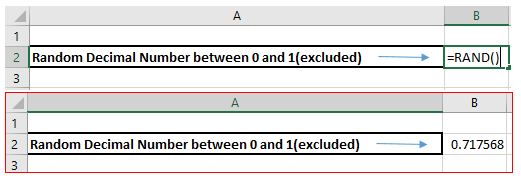
We must type =RAND() in the cell and press Enter. The value will change whenever any change is made in the sheet.
How To Generate Random Numbers In Excel For More Than One Cell?
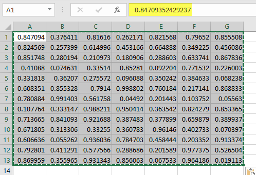
If we want to generate random numbers in Excel for more than one cell, then we need:
- First, select the required range, type =RAND(), and press Ctrl+Enter to give us the values.
How to Stop Recalculation of Random Numbers in Excel?
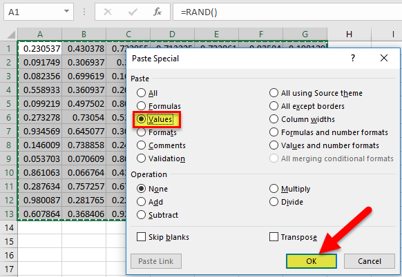
As the RAND function recalculates, if any change in the sheet is made, we must copy and then paste the formulas as values if we do not want values to be changed every time. For this, we need to paste the values of the RAND() function using Paste Special so that it would no longer be a result of the “RAND ()” function. It will not be recalculated.
To do this,
- We need to make the selection of the values.
- Press the Ctrl+C keys to copy the values.

- Without changing the selection, press the Alt+Ctrl+V keys to open the Paste Special dialog box.
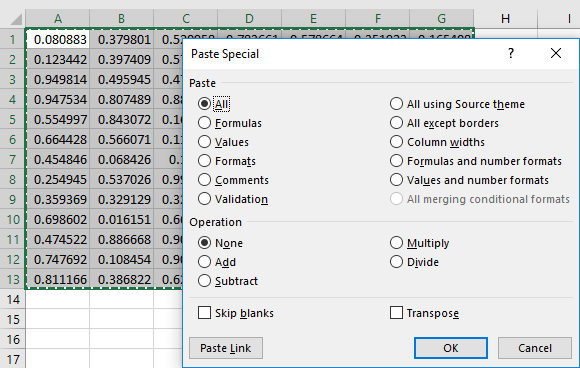
- Choose Values from the options and click on OK.
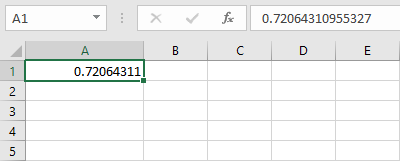
We can see that the value in the formula bar is the value itself, not the RAND() function. Now, these are only values.
There is one more way to get the value, only not the function as a result, but that is only for one cell. If we want the value the very first time, not the function, then the steps are:
- First, type =RAND() in the formula bar, press F9, and press the Enter key.
After pressing F9, we get the value only.
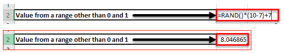
Value From A Different Range Other Than 0 And 1 Using RAND()
As the RAND function returns a random decimal number between 0 and 1 only, if we want the value from a different range, then we can use the following function:
Let ‘a’ be the start point.
And ‘b’ be the end point
The function would be ‘RAND()*(b-a)+a’
For example, if we have 7 as “a” and 10 as “b,” then the formula would be “=RAND()*(10-7)+7.”
RANDBETWEEN() Function
As the function’s name indicates, this function returns a random integer between given integers. Like the RAND() function, this function also recalculates when a workbook is changed or opened (volatile function).
The formula of the RANDBETWEEN Function is:
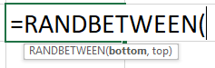
- Bottom: An integer representing the lower value of the range.
- Top: An integer representing the lower value of the range.
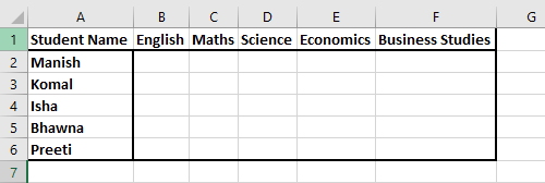
To generate random numbers in Excel for the students between 0 and 100, we will use the RANDBETWEEN function.
First, we must select the data, type the formula, =RANDBETWEEN(0,100), and press the Ctrl + Enter keys. You can prefer the below-given screenshot.
As values will recalculate, we can only use Alt+Ctrl+V to open the Paste Special dialog box to paste as values.
Follow the steps given below in the screenshot.
Like the RAND() function, we can also type the RANDBETWEEN function in the formula bar, pressing F9 to convert the result into value, and then press the Enter key.
Important Things To Remember
- If the bottom is greater than the top, the RANDBETWEEN function will return #NUM! Error.
- If either of the supplied arguments is non-numeric, the function will return #VALUE! Error.
- Both RAND() and RANDBETWEEN() functions are volatile functions (recalculates). Hence, it increases the processing time and can slow down the workbook.
Random Numbers In Excel – Project 1
We can use the RANDBETWEEN() function for getting random dates between two dates.
We will be using two dates as the bottom and top arguments.

After making the selection, we need to copy down the formula using the shortcut (Ctrl+D).

We can change the start date (D1) and end date (E1) to change the top and bottom values for the function.
Random Numbers In Excel – Project 2 – Head And Tail
To randomly choose head and tail, we can use the CHOOSE function in excel with the RANDBETWEEN function.

We need to copy the formula into the next and next cell every time in the game, and Head and Tail will come randomly.
Random Numbers In Excel – Project 3 – Region Allocation
Many times, we have to imagine and create data for various examples. For example, suppose we have data for sales, and we need to allocate three different regions to every sale transaction.
Then, we can use the RANDBETWEEN function with the CHOOSE function.

We can drag the same for the remaining cells.
Random Numbers In Excel – Project 4 – Creating Ludo Dice
Using the RANDBETWEEN function, we can also create dice for Ludo. We need to use the RANDBETWEEN function in Excel VBA for the same. Please follow the below steps:
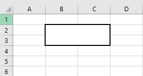
- Merge the four cells (B2:C3) using Home Tab → Alignment Group → Merge & Center.
- Apply the border to the merged cell using the shortcut key (ALT+H+B+T) by pressing one key after another.
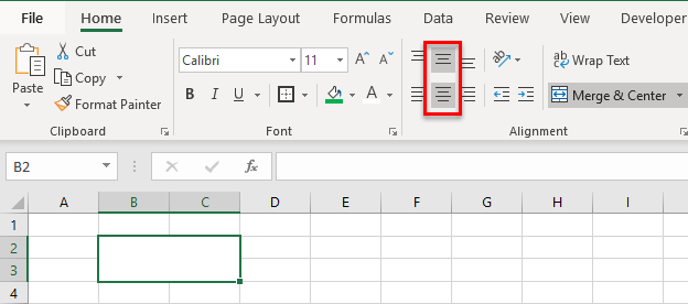
- Center and middle align the value using Home Tab → Alignment Group → Center and Middle Align commands.
- To create the button, use Developer tab → Controls Group → Insert → Command Button
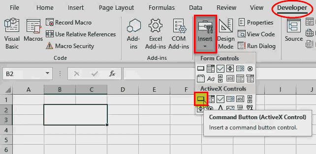
- Create the button and choose View Code from the Controls group on Developer.

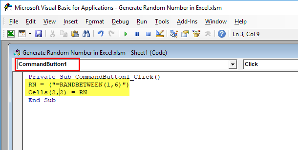
- After choosing CommandButton1 from the dropdown, paste the following code:
RN = (“=RANDBETWEEN(1,6)”)
Cells(2, 2) = RN
Please save the file using the .xlsm extension as we have used the VBA code in the workbook. After coming to the Excel window, deactivate the Design Mode.
Now, whenever we click the button, we get a random value between 1 and 6.
Frequently Asked Questions (FAQs)
1. What is Random Numbers in excel?
Random Numbers in excel is a built-in function used to generate random values. It is used when we have to calculate sample evaluation for random values.
2. What are the two functions used to generate random numbers in excel?
In excel, we can generate numbers using two functions. They are: =RAND() and =RANDBETWEEN().
The =RAND() provides us with any value from the range 0 to 1, whereas the =RANDBETWEEN() function takes input from the user for an arbitrary number range.
3. How to use RAND function in excel?
RAND() generates random numbers between 0 to 1.
For example, consider the below image where we have inserted the RAND() in a blank cell.

As soon as we press Enter¸ we can see that the function has generated a random number below 1 as shown in the below image.

Similarly, we can generate random numbers between 0 to 1, using random numbers in excel function.
Recommended Articles
This article is a guide to Random Numbers in Excel. Here, we discuss generating random numbers in Excel using the RAND() and RANDBETWEEN functions along with multiple projects and downloadable Excel templates. You may also look at these useful functions in Excel: –
- Randomize List in Excel
- Auto Number in Excel
- VBA Random Number
- RAND Function in Excel
There may be cases when you need to generate random numbers in Excel.
For example, to select random winners from a list or to get a random list of numbers for data analysis or to create random groups of students in class.
In this tutorial, you will learn how to generate random numbers in Excel (with and without repetitions).
Generate Random Numbers in Excel
There are two worksheet functions that are meant to generate random numbers in Excel: RAND and RANDBETWEEN.
- RANDBETWEEN function would give you the random numbers, but there is a high possibility of repeats in the result.
- RAND function is more likely to give you a result without repetitions. However, it only gives random numbers between 0 and 1. It can be used with RANK to generate unique random numbers in Excel (as shown later in this tutorial).
Generate Random Numbers using RANDBETWEEN function in Excel
Excel RANDBETWEEN function generates a set of integer random numbers between the two specified numbers.
RANDBETWEEN function takes two arguments – the Bottom value and the top value. It will give you an integer number between the two specified numbers only.
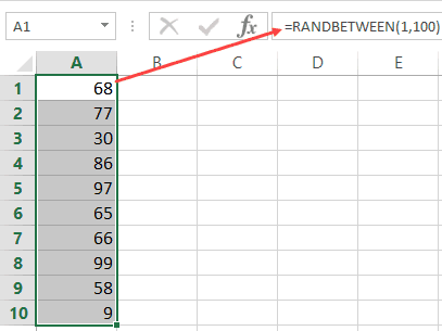
For example, suppose I want to generate 10 random numbers between 1 and 100.
Here are the steps to generate random numbers using RANDBETWEEN:
- Select the cell in which you want to get the random numbers.
- In the active cell, enter =RANDBETWEEN(1,100).
- Hold the Control key and Press Enter.
This will instantly give me 10 random numbers in the selected cells.
While RANDBETWEEN makes it easy to get integers between the specified numbers, there is a high chance of repetition in the result.
For example, when I use the RANDBETWEEN function to get 10 random numbers and use the formula =RANDBETWEEN(1,10), it gives me a couple of duplicates.
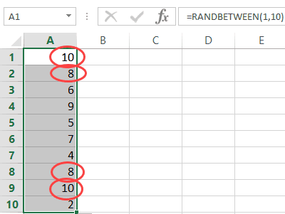
If you’re OK with duplicates, RANDBETWEEN is the easiest way to generate random numbers in Excel.
Note that RANDBETWEEN is a volatile function and recalculates every time there is a change in the worksheet. To avoid getting the random numbers recalculate, again and again, convert the result of the formula to values.
Generate Unique Random Numbers using RAND and RANK function in Excel
I tested the RAND function multiple times and didn’t find duplicate values. But as a caution, I recommend you check for duplicate values when you use this function.
Suppose I want to generate 10 random numbers in Excel (without repeats).
Here are the steps to generate random numbers in Excel without repetition:
Now you can use the values in column B as the random numbers.
Note: RAND is a volatile formula and would recalculate every time there is any change in the worksheet. Make sure you have converted all the RAND function results to values.
Caution: While I checked and didn’t find repetitions in the result of the RAND function, I still recommend you check once you have generated these numbers. You can use Conditional Formatting to highlight duplicates or use the Remove Duplicate option to get rid of it.
You May Also Like the Following Excel Tutorials:
- Automatically Sort Data in Alphabetical Order using Formula.
- Random Group Generator Template
- How to Shuffle a List of Items/Names in Excel?
- How to Do Factorial (!) in Excel (FACT function)