
Постановка задачи
Давайте разберем красивое решение для одной из весьма стандартных ситуаций, с которой рано или поздно сталкивается большинство пользователей Excel: нужно быстро и автоматически собрать данные из большого количества файлов в одну итоговую таблицу.
Предположим, что у нас есть вот такая папка, в которой содержится несколько файлов с данными из филиалов-городов:

Количество файлов роли не играет и может меняться в будущем. В каждом файле есть лист с именем Продажи, где расположена таблица с данными:

Количество строк (заказов) в таблицах, само-собой, разное, но набор столбцов везде стандартный.
Задача: собрать данные из всех файлов в одну книгу с последующим автоматическим обновлением при добавлении-удалении файлов-городов или строк в таблицах. По итоговой консолидированной таблице затем можно будет строить любые отчеты, сводные таблицы, фильтровать-сортировать данные и т.д. Главное — суметь собрать.
Подбираем оружие
Для решения нам потребуется последняя версия Excel 2016 (в нее нужный функционал уже встроен по умолчанию) или предыдущие версии Excel 2010-2013 с установленной бесплатной надстройкой Power Query от Microsoft (скачать ее можно здесь). Power Query — это супергибкий и супермощный инструмент для загрузки в Excel данных из внешнего мира с последующей их зачисткой и обработкой. Power Query поддерживает практически все существующие источники данных — от текстовых файлов до SQL и даже Facebook 
Если у вас нет Excel 2013 или 2016, то дальше можно не читать (шучу). В более древних версиях Excel подобную задачу можно реализовать только программированием макроса на Visual Basic (что весьма непросто для начинающих) или монотонным ручным копированием (что долго и порождает ошибки).
Шаг 1. Импортируем один файл как образец
Для начала давайте импортируем данные из одной книги в качестве примера, чтобы Excel «подхватил идею». Для этого создайте новую пустую книгу и…
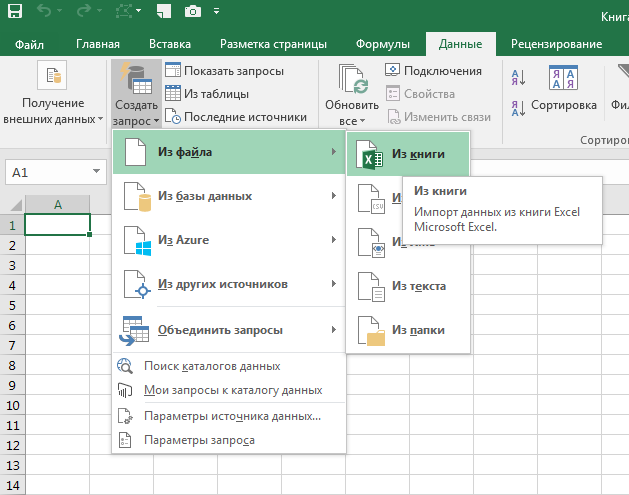
- если у вас Excel 2016, то откройте вкладку Данные и выберите Создать запрос — Из файла — Из книги (Data — New Query- From file — From Excel)
- если у вас Excel 2010-2013 с установленной надстройкой Power Query, то откройте вкладку Power Query и выберите на ней Из файла — Из книги (From file — From Excel)
Затем в открывшемся окне переходим в нашу папку с отчетами и выбираем любой из файлов-городов (не играет роли какой именно, т.к. они все типовые). Через пару секунд должно появиться окно Навигатор, где нужно в левой части выбрать требуемый нам лист (Продажи), а в правой отобразится его содержимое:

Если нажать в правом нижнем углу этого окна кнопку Загрузить (Load), то таблица будет сразу импортирована на лист в исходном виде. Для одиночного файла — это хорошо, но нам нужно загрузить много таких файлов, поэтому мы пойдем немного другим путем и жмем кнопку Правка (Edit). После этого должен в отдельном окне отобразиться редактор запросов Power Query с нашими данными из книги:

Это очень мощный инструмент, позволяющий «допилить» таблицу под нужный нам вид. Даже поверхностное описание всех его функций заняло бы под сотню страниц, но, если совсем кратко, то с помощью этого окна можно:
- отфильтровывать ненужные данные, пустые строки, строки с ошибками
- сортировать данные по одному или нескольким столбцам
- избавляться от повторов
- делить слипшийся текст по столбцам (по разделителям, количеству символов и т.д.)
- приводить текст в порядок (удалять лишние пробелы, исправлять регистр и т.д.)
- всячески преобразовывать типы данных (превращать числа как текст в нормальные числа и наоборот)
- транспонировать (поворачивать) таблицы и разворачивать двумерные кросс-таблицы в плоские
- добавлять к таблице дополнительные столбцы и использовать в них формулы и функции на встроенном в Power Query языке М.
- …
Для примера, давайте добавим к нашей таблице столбец с текстовым названием месяца, чтобы потом проще было строить отчеты сводных таблиц. Для этого щелкните правой кнопкой мыши по заголовку столбца Дата и выберите команду Дублировать столбец (Duplicate Column), а затем щелкните правой кнопкой мыши по заголовку появившегося столбца-дубликата и выберите команды Преобразование — Месяц — Название месяца:

Должен образоваться новый столбец с текстовыми названиями месяца для каждой строки. Дважды щелкнув по заголовку столбца, его можно переименовать из Копия Дата в более удобное Месяц, например.

Если в каких-то столбцах программа не совсем корректно распознала тип данных, то ей можно помочь, щелкнув по значку формата в левой части каждого столбца:

Исключить строки с ошибками или пустые строки, а также ненужных менеджеров или заказчиков можно с помощью простого фильтра:

Причем все выполненные преобразования фиксируются в правой панели, где их всегда можно откатить (крестик) или изменить их параметры (шестеренка):

Легко и изящно, не правда ли?
Шаг 2. Преобразуем наш запрос в функцию
Чтобы впоследствии повторить все сделанные преобразования данных для каждой импортируемой книги, нужно преобразовать наш созданный запрос в функцию, которая затем будет применяться, по очереди, ко всем нашим файлам. Сделать это, на самом деле, очень просто.
В редакторе запросов перейдите на вкладку Просмотр и нажмите кнопку Расширенный редактор (View — Advanced Editor). Должно открыться окно, где все наши предыдущие действия будут записаны в виде кода на языке М. Обратите внимание, что в коде жестко прописан путь к файлу, который мы импортировали для примера:

Теперь аккуратно вносим пару правок:

Смысл их прост: первая строка (filepath)=> превращает нашу процедуру в функцию с аргументом filepath, а ниже мы меняем фиксированный путь на значение этой переменной.
Все. Жмем на Готово и должны увидеть вот это:

Не пугайтесь, что пропали данные — на самом деле все ОК, все так и должно выглядеть Мы успешно создали нашу пользовательскую функцию, где запомнился весь алгоритм импорта и обработки данных без привязки к конкретному файлу. Осталось дать ей более понятное имя (например getData) на панели справа в поле Имя и можно жать Главная — Закрыть и загрузить (Home — Close and Load). Обратите внимание, что в коде жестко прописан путь к файлу, который мы импортировали для примера.. Вы вернетесь в основное окно Microsoft Excel, но справа должна появиться панель с созданным подключением к нашей функции:

Шаг 3. Собираем все файлы
Все самое сложное — позади, осталась приятная и легкая часть. Идем на вкладку Данные — Создать запрос — Из файла — Из папки (Data — New Query — From file — From folder) или, если у вас Excel 2010-2013, аналогично на вкладку Power Query. В появившемся окне указываем папку, где лежат все наши исходные файлы-города и жмем ОК. Следующим шагом должно открыться окно, где будут перечислены все найденные в этой папке (и ее подпапках) файлы Excel и детализация по каждому из них:

Жмем Изменить (Edit) и опять попадаем в знакомое окно редактора запросов.
Теперь нужно добавить к нашей таблице еще один столбец с нашей созданной функцией, которая «вытянет» данные из каждого файла. Для этого идем на вкладку Добавить столбец — Пользовательский столбец (Add Column — Add Custom Column) и в появившемся окне вводим нашу функцию getData, указав для ее в качестве аргумента полный путь к каждому файлу:

После нажатия на ОК созданный столбец должен добавиться к нашей таблице справа.
Теперь удалим все ненужные столбцы (как в Excel, с помощью правой кнопки мыши — Удалить), оставив только добавленный столбец и столбец с именем файла, т.к. это имя (а точнее — город) будет полезно иметь в итоговых данных для каждой строки.
А теперь «вау-момент» — щелкнем мышью по значку со своенным стрелками в правом верхнем углу добавленного столбца с нашей функцией:

… снимаем флажок Использовать исходное имя столбца как префикс (Use original column name as prefix)и жмем ОК. И наша функция подгрузит и обработает данные из каждого файла, следуя записанному алгоритму и собрав все в общую таблицу:

Для полной красоты можно еще убрать расширения .xlsx из первого столбца с именами файлов — стандартной заменой на «ничего» (правой кнопкой мыши по заголовку столбца — Заменить) и переименовать этот столбец в Город. А также подправить формат данных в столбце с датой.
Все! Жмем на Главной — Закрыть и загрузить (Home — Close & Load). Все собранные запросом данные по всем городам будут выгружены на текущий лист Excel в формате «умной таблицы»:

Созданное подключение и нашу функцию сборки не нужно никак отдельно сохранять — они сохраняются вместе с текущим файлом обычным образом.
В будущем, при любых изменениях в папке (добавлении-удалении городов) или в файлах (изменение количества строк) достаточно будет щелкнуть правой кнопкой мыши прямо по таблице или по запросу в правой панели и выбрать команду Обновить (Refresh) — Power Query «пересоберет» все данные заново за несколько секунд.
P.S.
Поправка. После январских обновлений 2017 года Power Query научился собирать Excel’евские книги сам, т.е. не нужно больше делать отдельную функцию — это происходит автоматически. Таким образом второй шаг из этой статьи уже не нужен и весь процесс становится заметно проще:
- Выбрать Создать запрос — Из файла — Из папки — Выбрать папку — ОК
- После появления списка файлов нажать Изменить
- В окне редактора запросов развернуть двойной стрелкой столбец Binary и выбрать имя листа, который нужно взять из каждого файла
И все! Песня!
Ссылки по теме
- Редизайн кросс-таблицы в плоскую, подходящую для построения сводных таблиц
- Построение анимированной пузырьковой диаграммы в Power View
- Макрос для сборки листов из разных файлов Excel в один
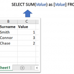
You can use Microsoft Query in Excel to retrieve data from an Excel Workbook as well as External Data Sources using SQL SELECT Statements. Excel Queries created this way can be refreshed and rerun making them a comfortable and efficient tool in Excel.
Microsoft Query allows you use SQL directly in Microsoft Excel, treating Sheets as tables against which you can run Select statements with JOINs, UNIONs and more. Often Microsoft Query statements will be more efficient than Excel formulas or a VBA Macro. A Microsoft Query (aka MS Query, aka Excel Query) is in fact an SQL SELECT Statement. Excel as well as Access use Windows ACE.OLEDB or JET.OLEDB providers to run queries. Its an incredible often untapped tool underestimated by many users!
What can I do with MS Query?
 Using MS Query in Excel you can extract data from various sources such as:
- Excel Files – you can extract data from External Excel files as well as run a SELECT query on your current Workbook
- Access – you can extract data from Access Database files
- MS SQL Server – you can extract data from Microsoft SQL Server Tables
- CSV and Text – you can upload CSV or tabular Text files
Step by Step – Microsoft Query in Excel
In this step by step tutorial I will show you how to create an Microsoft Query to extract data from either you current Workbook or an external Excel file.
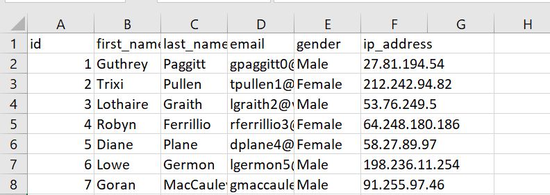
I will extract data from an External Excel file called MOCK DATA.xlsx. In this file I have a list of Male/Female mock-up customers. I will want to create a simple query to calculate how many are Male and how many Female.
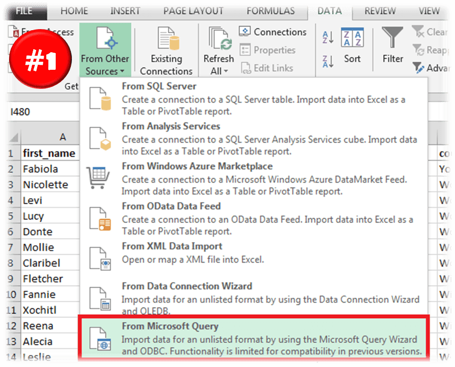
Open the MS Query (from Other Sources) wizard
Go to the DATA Ribbon Tab and click From Other Sources. Select the last option From Microsoft Query.
Select the Data Source
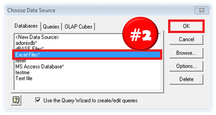 Next we need to specify the Data Source for our Microsoft Query. Select Excel Files to proceed.
Select Excel Source File
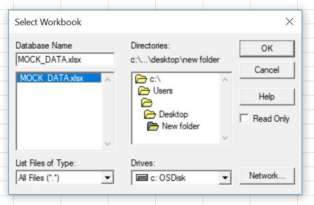 Now we need to select the Excel file that will be the source for our Microsoft Query. In my example I will select my current Workbook, the same from which I am creating my MS Query.
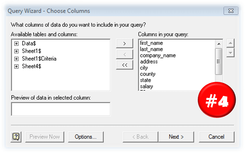
Select Columns for your MS Query
The Wizard now asks you to select Columns for your MS Query. If you plan to modify the MS Query manually later simply click OK. Otherwise select your Columns.
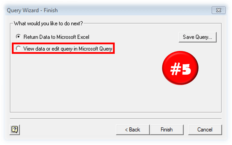
Return Query or Edit Query
 Now you have two options:
- Return Data to Microsoft Excel – this will return your query results to Excel and complete the Wizard
- View data or edit query in Microsoft Query – this will open the Microsoft Query window and allow you to modify you Microsoft Query
Optional: Edit Query
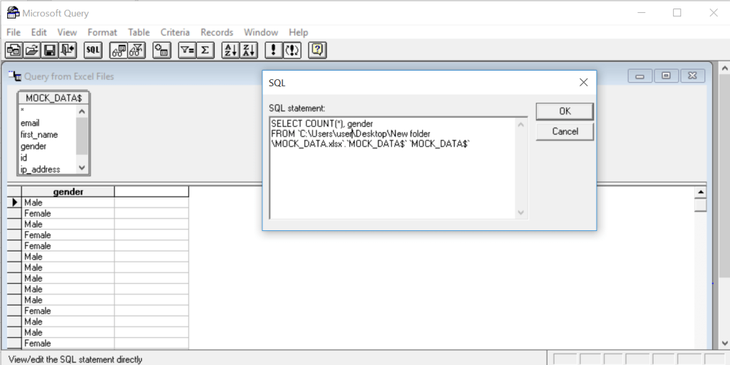 If you select the View data or edit query in Microsoft Query option you can now open the SQL Edit Query window by hitting the SQL button. When you are done hit the return button (the one with the open door).
Import Data
When you are done modifying your SQL statement (as I in previous step). Click the Return data button in the Microsoft Query window.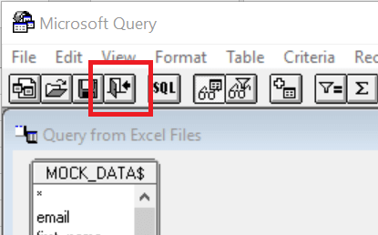
This should open the Import Data window which allows you to select when the data is to be dumped.
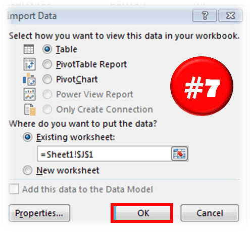 Lastly, when you are done click OK on the Import Data window to complete running the query. You should see the result of the query as a new Excel table:
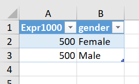
As in the window above I have calculated how many of the records in the original table where Male and how many Female.
AS you can see there are quite a lot of steps needed to achieve something potentially pretty simple. Hence there are a couple of alternatives thanks to the power of VBA Macro….
MS Query – Create with VBA
If you don’t want to use the SQL AddIn another way is to create these queries using a VBA Macro. Below is a quick macro that will allow you write your query in a simple VBA InputBox at the selected range in your worksheet.
Just use my VBA Code Snippet:
Sub ExecuteSQL()
    Attribute ExecuteSQL.VB_ProcData.VB_Invoke_Func = "Sn14"
    'AnalystCave.com
    On Error GoTo ErrorHandl
    Dim SQL As String, sConn As String, qt As QueryTable
    SQL = InputBox("Provide your SQL Query", "Run SQL Query")
    If SQL = vbNullString Then Exit Sub
    sConn = "OLEDB;Provider=Microsoft.ACE.OLEDB.12.0;;Password=;User ID=Admin;Data Source=" & _
        ThisWorkbook.Path & "/" & ThisWorkbook.Name & ";" & _
        "Mode=Share Deny Write;Extended Properties=""Excel 12.0 Xml;HDR=YES"";"
    Set qt = ActiveCell.Worksheet.QueryTables.Add(Connection:=sConn, Destination:=ActiveCell)
    With qt
        .CommandType = xlCmdSql
        .CommandText = SQL
        .Name = Int((1000000000 - 1 + 1) * Rnd + 1)
        .RefreshStyle = xlOverwriteCells
        .Refresh BackgroundQuery:=False
    End With
    Exit Sub
ErrorHandl: MsgBox "Error: " & Err.Description: Err.Clear
End Sub
Just create a New VBA Module and paste the code above. You can run it hitting the CTRL+SHIFT+S Keyboardshortcut or Add the Macro to your Quick Access Toolbar.
Learning SQL with Excel
Creating MS Queries is one thing, but you need to have a pretty good grasp of the SQL language to be able to use it’s true potential. I recommend using a simple Excel database (like Northwind) and practicing various queries with JOINs.
Alternatives in Excel – Power Query
Another way to run queries is to use Microsoft Power Query (also known in Excel 2016 and up as Get and Transform). The AddIn provided by Microsoft does require knowledge of the SQL Language, rather allowing you to click your way through the data you want to tranform.
MS Query vs Power Query Conclusions
MS Query Pros: Power Query is an awesome tool, however, it doesn’t entirely invalidate Microsoft Queries. What is more, sometimes using Microsoft Queries is quicker and more convenient and here is why:
- Microsoft Queries are more efficient when you know SQL. While you can click your way through to Transform Data via Power Query someone who knows SQL will likely be much quicker in writing a suitable SELECT query
- You can’t re-run Power Queries without the AddIn. While this obviously will be a less valid statement probably in a couple of years (in newer Excel versions), currently if you don’t have the AddIn you won’t be able to edit or re-run Queries created in Power Query
MS Query Cons: Microsoft Query falls short of the Power Query AddIn in some other aspects however:
- Power Query has a more convenient user interface. While Power Queries are relatively easy to create, the MS Query Wizard is like a website from the 90’s
- Power Query stacks operations on top of each other allowing more convenient changes. While an MS Query works or just doesn’t compile, the Power Query stacks each transform operation providing visibility into your Data Transformation task, and making it easier to add / remove operations
In short I encourage learning Power Query if you don’t feel comfortable around SQL. If you are advanced in SQL I think you will find using good ole Microsoft Queries more convenient. I would compare this to the Age-Old discussion between Command Line devs vs GUI devs…
Are you dealing with data from a bunch of different places and combine them on a regular basis to do analysis or reporting? Excel Power Query may be the solution you’re looking for! The best thing about this tool is that you can fully automate your data loading and cleaning procedures with a click of a button.
In this tutorial, you’ll learn what Power Query can do and how powerful its features really are. We also provide some practical examples that you can follow to understand basic data transformations using this tool. Let’s get started!
What is Power Query in Excel?
Power Query is a business intelligence tool in Excel used to carry out the ETL (Extract, Transform, and Load) process. This process involves getting data from a source, transforming it, then placing it to a destination for analysis. ETL is known as a crucial step in building a data warehouse, but actually, you’re doing ETL-like processes even if you’re just doing a weekly or monthly report.
What can Power Query do?
With Power Query, everyone can deliver meaningful insight quickly using Excel. There was a time when BI processes required dedicated teams of IT specialists, but not anymore. You can use Power Query as part of your self-service ETL solution to do the following tasks:
#1. Extract (connect and get) data from a source
Power Query allows you to connect instantly with a wide range of data in different formats and locations. Whether your data is in CSV, XML, JSON, or PDF formats, that’s not a problem. Your organization stores data in Azure SQL Database, IBM DB2, Oracle, or PostgreSQL? You can easily access them. Even if you use platforms such as Salesforce and MS Dynamics 365, just connect straight away without hassle!
#2. Transform your data to make it ready for analysis
After connecting to a data source, you may need to modify the data in several ways. Data transformation is the area where Power Query shines. This tool allows for a range of operations, from simple data transformation tasks to the most complex data restructuring challenges, in just a few clicks.
Examples of data transformation tasks:
- Data cleaning: Remove duplicates, change data types and formatting, filter rows, split columns, and pivot/unpivot columns.
- Data integration: Join or split source tables, add lookup keys, and aggregate data.
- Data enrichment: Extend the source data by creating calculated columns.
The ones mentioned above merely scratches the surface of all that Power Query can do to transform your data. The best thing about this tool is that you can automate those data transformation tasks using a code-free interface — without macro or VBA codes.
#3. Load transformed data into a worksheet or the Data Model
After your data is clean and ready for analysis, Power Query Excel gives you options to load your data into one or both of these destinations:
- A worksheet. By default, Power Query lands the output data directly in a new worksheet inside your Excel file. If you want, you can place data from each source into a separate worksheet and then do whatever you want with it, just as if it were “normal” Excel data.
- The Data Model. Your data is compressed and stored in memory. With this option, you can work with millions, tens of millions, even hundreds of millions of rows of data, exceeding the 1,048,576 row limit of an Excel worksheet!
The Data Model is normally used as the basis for pivot table output in Excel. Thus, it’s also referred to as the Power Pivot Data Model. This article won’t be covering the Data Model and Power Pivot in more detail, as those are broad subjects.
Why use Excel Power Query?
Not only does Power Query allow you to get and transform your data, but this tool also records all the steps applied.
You can refresh all the processes such as re-import the source data, reapply all the data filtering, sorting, and other transformations that you defined — in a single click. So, once all of that’s set up, you don’t need to create it again. Of course, you can also go back and edit each step, and even add steps in between.
This is all done within a tool you’re already familiar with: Excel.
Power Query in different versions of Excel
Power Query for Excel was initially released as an add-in to download and install for Excel 2010 and 2013. After you add Power Query to Excel, a new tab named Power Query will appear in the Excel ribbon.
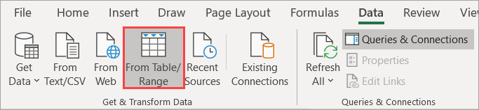
This tool was fully integrated into Excel by the 2016 version and accessed under the Get & Transform section in the Data tab. So if you use the latest versions of Excel, you already have Power Query integrated within Excel.
The following image summarizes where you can find Power Query in different versions of Excel. Please note that each build of Excel may be slightly different — so you might see slightly different icons.
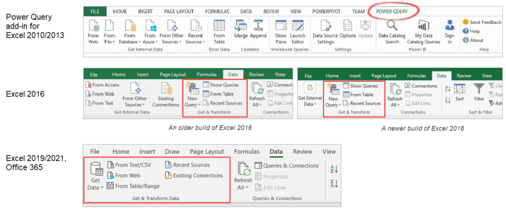
We use Office 365 in this tutorial, however, you can follow the steps described in this article with earlier versions of the product. The entry point into Power Query may be different, but this should not cause any significant difficulties.
Excel Power Query: Download sample files
We provide a small set of sample data used in the examples throughout this article. Just download files from this link to make it easier for you to follow along:
Download sample files
After that, put the CSVs in a folder, for example in “D:/Power Query/Sample files”.
How to use Power Query to GET and LOAD data into Excel
Let’s begin with a quick overview of Power Query’s list of data sources. After that, we’ll get some data into Excel and look into more detail about the Power Query interface.
Power Query list of data sources
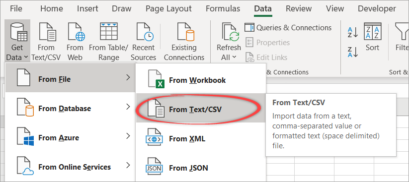
Go to the Data tab and locate Power Query in the Get & Transform Data section. Click on the Get Data button — you will see a dropdown menu to select your data source:

Please note that the range of available Power Query data sources will depend on the version of Excel that you are using.
Data source options
- From File: Excel, TXT/CSV, XML, JSON, and PDF.
- From Database: SQL Server, Access, Oracle, DB2, MySQL, PostgreSQL, Sybase, Teradata, and SAP Hana.
- From Azure: Azure SQL Database, Azure Synapse Analytics, Azure HDInsight (HDFS), Azure Blob, Azure Table, and Azure Data Lake Storage.
- From Online Services: Sharepoint Online, Exchange Online, Dynamics 365, Salesforce Objects, and Salesforce Reports.
- From Other Sources: Excel Table/Range, Web, OData Feed, ODBC, OLEDB, Active Directory, etc.
If you take a closer look at the Get Data options, you will find that there are currently around 40 data sources for which Power Query connectors are available. However, even this number is small compared to the number of potential data sources out there.
What can you do if your data source is not among those currently available?
One solution is by using a generic data connector such as OData Feed, OLE DB, and ODBC. Another solution is to use an integration tool to help you seamlessly connect and get data from external apps into Excel. An example of this is by using Coupler.io, which is a solution to import data from various apps such as Airtable, Shopify, Jira, QuickBooks, Pipedrive, Hubspot, and more!
Check out the complete list of Coupler.io’s Excel integrations.
A simple example: Get data from CSV files into Excel using Power Query
In the following example, we will import data from two downloaded CSV files one by one and load them into new worksheets.
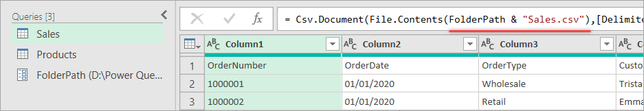
First, we’ll show you how to get and load Sales.csv directly into a new worksheet. After that, we’ll show you how to import Products.csv and open it in the Power Query Editor before loading it. Here are the steps:
- Open a new blank Excel workbook.
- Click the Data tab, then click the Get Data button in the Get & Transform Data section.
- In the dropdown, select From File > From TXT/CVS.
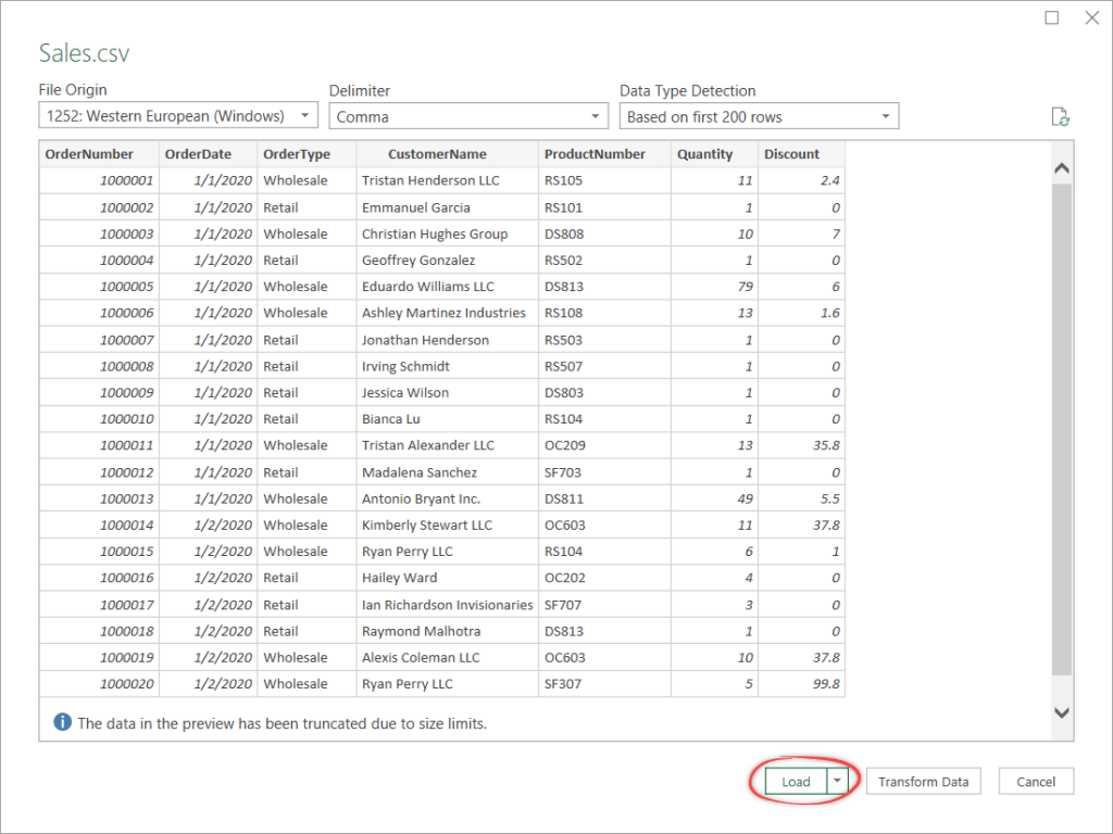
- Browse the folder where you downloaded the sample files. Then, select Sales.csv and click Import.

- In the Preview window, click Load to load the data into a new worksheet.
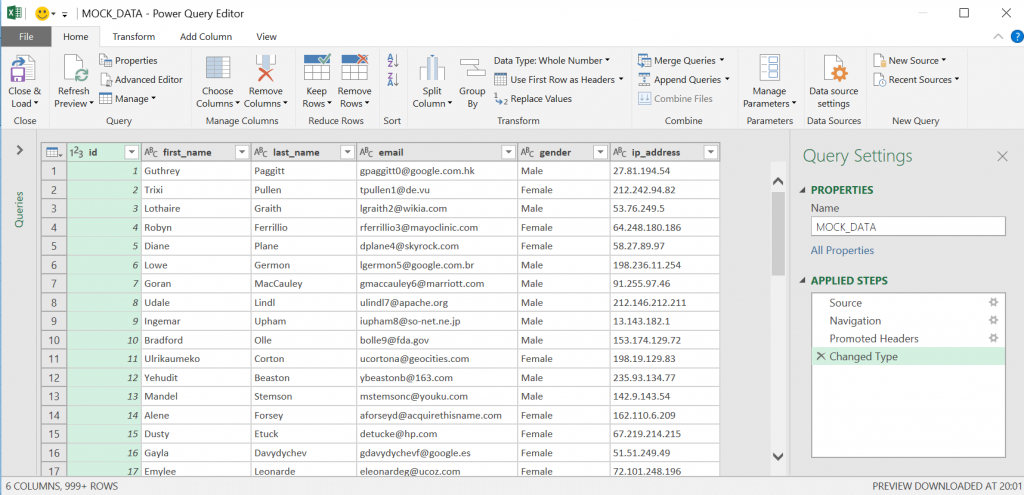
You will see a new worksheet inside the current workbook, as shown in the below screenshot. Your external data is now an Excel table. On the right pane, notice that there is a query to your data source listed there.

- Import Products.csv by repeating Steps 1-4 above, but this time, don’t forget to select Products.csv instead of Sales.csv.
- In the Preview window, click Transform Data.
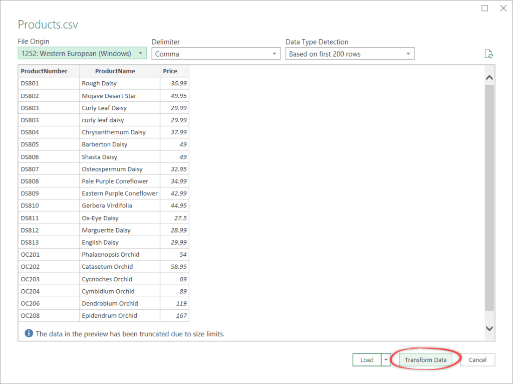
This will open the Power Query Editor as shown in the following screenshot:

As you can see, clicking Transform Data will bring you to a different, separate interface called Power Query Editor. This editor allows you to transform your data before loading it into a new worksheet.
We’ll cover more detail about the Power Query Editor in the next section. For now, let’s not do any data transformations here. We’ll continue to load the products data into a new worksheet from this editor.
- Click the small triangle icon in the Close & Load button in the Home tab. Select the first option in the dropdown.

Note: If you choose the second option, you’ll get more options to load your data — more about this in the Load To… options section.
As the final result, you will see a new worksheet created containing the Products table. If you notice, there are two queries listed on the right pane: Sales and Products.

You’ve learned how to get and load two CSV files directly to Excel using Power Query. By the way, you can do something similar using Coupler.io as it includes a CSV to Excel integration as well. You can even set up automatic data refresh on schedule, such as hourly, weekly, and monthly.
Try Coupler.io for free with the seamless Excel integration
Load To… options in Excel Power Query
As explained previously, Power Query provides you with two options to load data: to a worksheet and/or data model. If you want to load data into a worksheet, there are several variations if you choose the Load To… option:

As shown in the above dialog, you can:
- Load into an Excel named table (the default)
- Load into a pivot table based on the source data
- Load into a pivot chart based on the source data
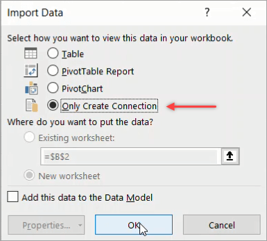
- Only create a connection to the data, but do not load it yet
Notice that on top of this, you have the choice of whether you want to create the table of data, pivot table, or pivot chart in an existing or new worksheet.
If you also want to add the data to the Data Model, tick the Add this data to the Data Model checkbox.
Excel Power Query Editor
The Power Query Editor is a separate interface from Excel. All of your data transformations will happen in this editor, which can be launched in one of these two ways:
- Click the Get Data button then select Launch Power Query Editor…
- Double-click a query listed in the Queries & Connections pane.

Here are the six main elements of Power Query Editor:

- The Ribbon. It has 5 main tabs: File, Home, Transform, Add Column, and View.
- Query List. This pane contains all the queries that have been added to the current workbook. You can navigate to any query from this area to begin editing it.
- Data Preview. This area is where you can see a sample of the data for a selected query.
- Formula Bar. This area shows the M code of the current transformation step. Power Query records each of your transformation steps into the M code that you can see in this formula bar. Most of the time, you don’t need to use the M language directly at all.
- Properties. This is where you can see and edit the properties of your query. For example, you can rename your query, add a description to it, and enable fast data loading.
- Applied Steps. This area contains a list of steps used to transform data.
How to use Power Query to TRANSFORM data in Excel
The range of transformations that Power Query offers are wide and varied. It can be initially daunting if you’re unfamiliar with the feature set available in this tool, but don’t worry! We’ve selected some simple, practical examples for you:
Excel Power Query: Remove duplicates
An external source of data might not be as flawless as you expect. The presence of duplicates is one of the most annoying characteristics of poor quality data.
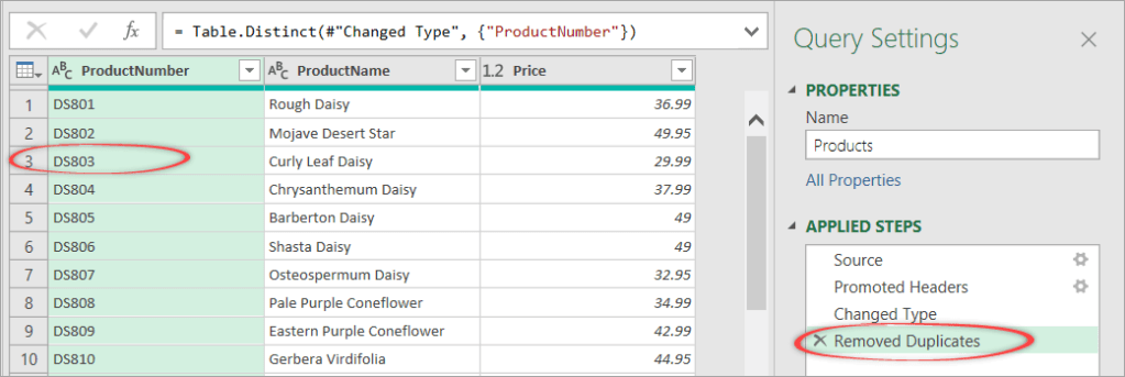
If you look closely at the Products table, you’ll notice two products with ProductNumber DS803.

To remove the above duplicates, follow the steps below:
- Launch the Power Query Editor and make sure to select the Products query.

- In the Home tab, click Remove Rows > Remove Duplicates.

- Notice that one of the rows with ProductNumber DS803 is now removed and a step added in the APPLIED STEPS pane:
- Click the Close & Load button. This will refresh the Products table in your worksheet.
Excel Power Query: Create parameters for folder paths
In the Power Query Editor, let’s open the Products query and click on the first row “Source” in the APPLIED STEPS. You will see a hard-coded file path like shown below:

If you check on the Sales query, you’ll notice that it also uses a fixed value for the file path, i.e., D:Power QuerySample filesSales.csv
Changing the folder path to use a parameter can be a time-saver in the future. In case you need to move your files to another folder later, you’ll only need to change the parameter value once.
Let’s do the following steps to replace the hard-coded folder path with a parameter:
- In the Home tab, click Manage Parameters > New Parameter.

- Create a new parameter using the following details, then click OK.
- Name:
FolderPath - Required:
✔ - Type:
Text - Suggested Values:
Any value - Current Value:
D:Power QuerySample files
- Name:

- Select the Products query, then click “Source” in the APPLIED STEPS.
- In the formula bar, replace the folder path to use the FolderPath parameter:
FolderPath & "Products.csv"

- Now, select the Sales query, then click “Source” in the APPLIED STEPS.
- In the formula bar, replace the folder path to use the FolderPath parameter:
FolderPath & "Sales.csv"
Now, you’ve changed the file path of both queries to use the FolderPath parameter. Please be aware that the code in the formula bar is case-sensitive. Also, notice that you don’t need to enclose parameters with double quotes.
Excel Power Query: Adding a conditional column with IF statement
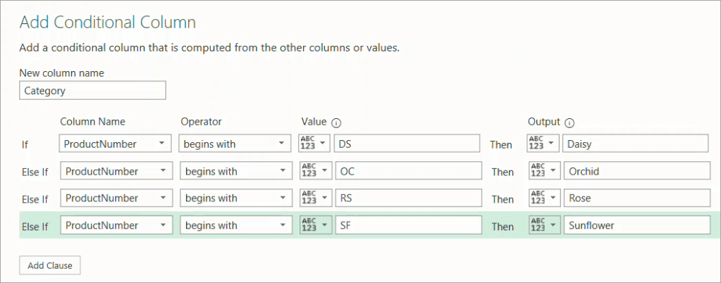
Suppose you want to create a new column, i.e., Category in the Products query, that tells you which category each product belongs to. The first 2 digits of the product number identify the product category based on the following rules:
- Product number begins with “DS” → Daisy
- Product number begins with “OC” → Orchid
- Product number begins with “RS” → Rose
- Product number begins with “SF” → Sunflower
Here’s how you can add the Category column:
- Open the Power Query Editor and select the Products query.
- Click the Add Column tab, then click Conditional Column.

- In the “Add Conditional Column” dialog that appears, enter the following details, then click OK when done.
- Click File > Close & Load.
- Notice that your worksheet containing the Products table will have the new Category column, as shown below:

Excel Power Query: Drill-down to create parameters from cell
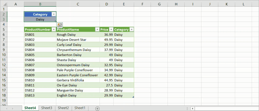
Suppose you want to be able to filter products by category from a cell as shown in the below image:

To pass the value from cell B3 to the query and use it to filter the products, follow the steps below:
- Create a new worksheet, e.g. Sheet4, then add the following details:
- Cell B2: A text “Category”.
- Cell B3: A dropdown containing a list of product categories: Daisy, Orchid, Rose, and Sunflower. You can create the dropdown using Data > Data Validation with details as follows:

- Click Data > From Table/Range.
- In the “Create Table” dialog, enter the following details, then click OK.
- Table range:
=$B$2:$B$3 - My table has headers:
✔
- Table range:

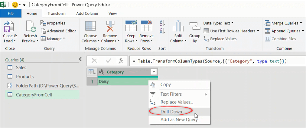
- In the Power Query Editor that opens, rename the new query to CategoryFromCell.

- Right-click on the data and select Drill Down.
- Click File > Close & Load To…
- In the “Import Data” dialog, select Only Create Connection.
- Reopen the Power Query Editor.
- Right-click on the Products query and select Duplicate. Rename the new query as ProductsByCategory.

- Add a filter by category by selecting the small triangle icon in the Category column, then choose Text Filters > Equals.
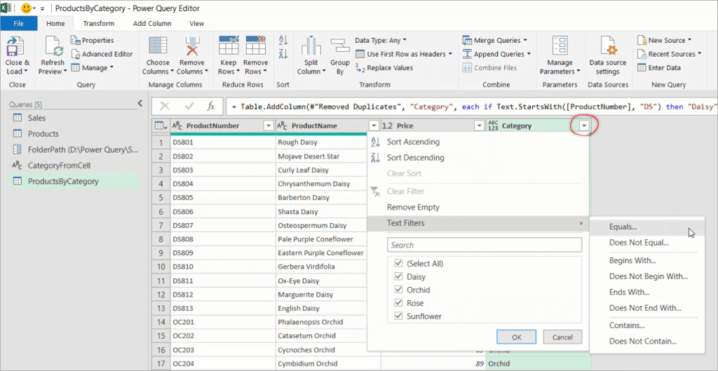
- In the Filter Rows dialog, type “Daisy”, then click OK.

- In the Formula Bar, change the text “Daisy” to use the CategoryFromCell parameter.

- Click File > Close & Load To… Then, in the “Import Data” dialog, select to load to the existing worksheet Sheet4!$B$5 and click OK when done.

Your final worksheet will look like this below. Test by changing the dropdown value to “Rose”, then click the Refresh All button.
Excel Power Query: Merge tables
Merging queries allows you to join tables based on a key column. This is like using VLOOKUP Excel. For example, here we’re going to merge the Sales and Products queries into one. We will retrieve columns from the Products table (the lookup table) and pull them into the Sales table.
Here are the steps:
- Launch the Power Query Editor and select the Sales query.
- Click Merge Queries in the Home tab, then select Merge Queries as New.

Note: As you can see, you have two options for merging. You can either overwrite the current Sales query with additional columns or merge two queries as a new one to keep your current Sales table unchanged.
- In the “Merge” dialog box, select Products as the second table. Then, select the ProductNumber column for both tables and click OK.

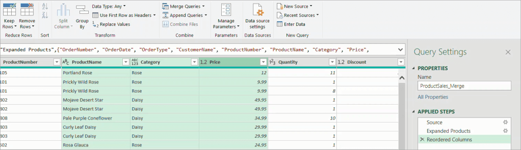
- If you want, rename the new query as ProductSales_Merge by changing the query name in the Properties pane.
- Expand the Products table and select ProductName, Price, and Category columns to include in the query.

- If you want, reorder the columns by moving them to the position you want, the same way you move columns in Excel.
Here’s an example after we moved the ProductNumber, Category, and Price columns before the Quantity and Discount columns.
- Click File > Close & Load to load the query into a new worksheet.
Excel Power Query: Using formulas
Suppose that in the ProductSales_Merge query, we want to add a new column OrderTotal which is calculated from other columns using this formula:
OrderTotal = Price * Quantity - DiscountTo do that, follow the steps below:
- Launch the Power Query Editor and select the ProductSales_Merge query.
- In the Add Column tab, click Custom Column.
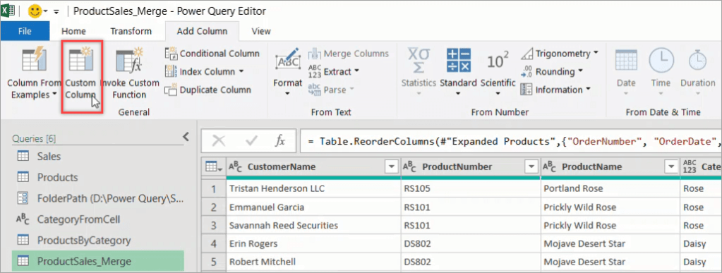
- In the “Custom Column” dialog that appears, enter the following details then click OK.
- New column name:
OrderTotal - Custom column formula: =
[Price] * [Quantity] - [Discount]
- New column name:
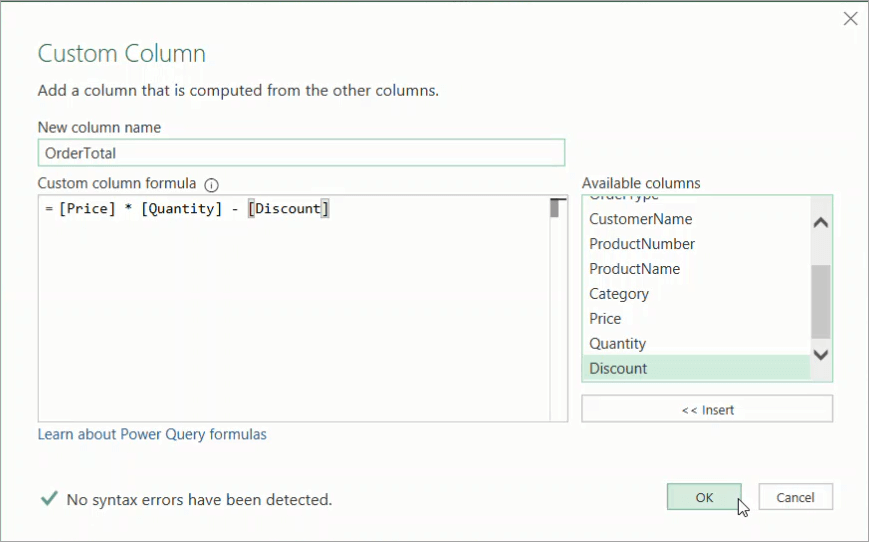
- Notice that a new column OrderTotal was added:

- Click File > Close & Load.
Excel Power Query: Using functions
In this last example, we’ll show you how to use functions in Power Query. We’ll add a new column Quarter that represents the number of the quarter from the order dates.
- Launch the Power Query Editor and select the ProductSales_Merge query.
- In the Add Column tab, click Custom Column.
- In the “Custom Column” dialog that appears, enter the following details, then click OK.
- New column name:
Quarter - Custom column formula:
= "Q"&Number.ToText(Date.QuarterOfYear([OrderDate]))
- New column name:

Explanation:
The Date.QuarterOfYear() function returns the number of the quarter (1-4) from a date, while the Number.ToText() function converts a number to text format.
- Notice that a new column Quarter was added.

- Click File > Close & Load to refresh your worksheet.
What’s next?
We’ve covered the basics of how you can use Excel Power Query to get, transform, and load data in Excel. We hope this tutorial has given you a great starting point working with Excel Power Query. Be sure to continue learning about Excel’s Data Model and Power Pivot if you want to master Business Intelligence using Excel.
In addition to importing your data into Excel, take a look at Coupler.io. This excellent integration tool may be a great solution you need if your data source is not among those currently available in Power Query. With this tool, you can import data from different apps into Excel — no coding required. You can also automate the import process on the schedule you want!
-

Senior analyst programmer

Back to Blog
Focus on your business
goals while we take care of your data!
Try Coupler.io

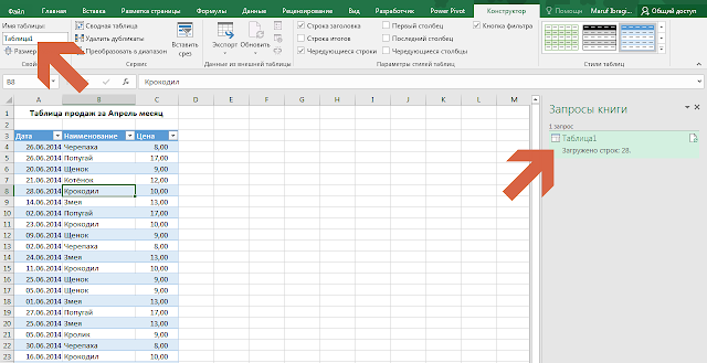
Процесс выгрузки данных из MS Excel в Power Query на первый взгляд достаточно прост — нужно лишь выделить любую ячейку внутри нужного диапазона данных и на вкладке Данные, выбрать команду Из таблицы.

При этом автоматически отобразится окно создания умной таблицы, после чего Excel создаст умную таблицу из указанного диапазона и сразу же загрузит находящиеся в этом диапазоне данные в среду Power Query.

Ни будем проводить каких-либо трансформаций а просто выберем команду Закрыть и загрузить. По умолчанию, данные загрузятся на новый лист в виде умной таблицы.
Если теперь мы вернёмся на предыдущий лист, то увидим что Excel автоматически преобразовал наш диапазон в умную таблицу и присвоил ей дефолтное имя Таблица1. Точно такое же имя было присвоено и созданному нами в Power Query запросу.
Вы также можете заранее преобразовать диапазон с данными в умную таблицу и присвоить ей более понятное имя после чего загружать эти данные в Power Query.
Получение данных из именованного диапазона
Может случиться так, что Вам необходимо сохранить исходное форматирование диапазона данных, следовательно преобразование этого диапазона в умную таблицу не желательно. В этом случае нужно выделить диапазон данных и на вкладке Формулы выбрать команду Присвоить имя. Откроется окно Создание имени, в котором нужно присвоить нашему диапазону подходящее имя, что преобразует его в именованный диапазон.

Теперь, если Вы попытаетесь загрузить данные в Power Query (опять же с помощью команды Из таблицы на вкладке Данные), Excel распознает именованный диапазон и уже не будет пытаться преобразовать его в умную таблицу.
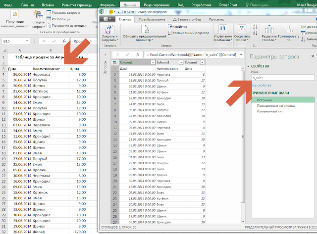
Получение данных с помощью пустого запроса
Если Ваша книга Excel уже содержит умные таблицы или именованные диапазоны, то Вы можете выбрать и загрузить их прямо из среды Power Query.
Для этого на вкладке Данные, в выпадающем списке Создать запрос выбираем Из других источников -> Пустой запрос. Откроется абсолютно пустое окно Power Query.

Далее в строке формул пишем:
=Excel.CurrentWorkbook()
Появится список всех умных таблиц и именованных диапазонов, содержащихся в текущей книге Excel. Находим нужную нам умную таблицу или именованный диапазон и жмём на зелёную надпись Table напротив их названия.

Получение данных из другой книги
Если же Вам не хочется возиться с созданием умных таблиц и именованных диапазонов, то Вы всё ещё можете получить данные исходного файла создавая запрос из другой книги.
Для этого нужно сохранить и закрыть исходную книгу и в новой книге Exel из выпадающего списка Создать запрос выбрать Из файла -> Из книги.
Далее находим и выбираем наш исходный файл, после чего откроется окно Навигатор со списком всех листов содержащихся в книге с данными. Выбрав нужный лист, Вы можете либо нажать на кнопу Изменить и продолжить работу с данными в среде Power Query, либо нажать на кнопку Загрузить и получить таблицу данных на новом листе текущей книги (или же указать другие параметры загрузки).

07 Aug 3 Ways to Perform an Excel SQL Query
Posted at 12:08h
in Excel VBA
0 Comments
Howdee! Excel is a great tool for performing data analysis. However, sometimes getting the data we need into Excel can be cumbersome and take a lot of time when going through other systems. You’re also at the mercy of how a disparate system exports data, and may need an additional step between exporting and getting the data into the format you need. If you have access to the database where the data is housed, you can circumvent these steps and create your own custom Excel SQL query.
To follow along with my below demos, you’ll need to have an instance of SQL server installed on your desktop. If you don’t, you can download the trial version, developer version, or free express version here. I’ll be working with the free developer version in this article. I’m also using a sample database that you can download here. The easiest way to install this is using SQL Server Management Studio (SSMS). That download is available here. Once you open SSMS, it should automatically detect your local server instance. You must ensure your SQL Server User is running as the “Local Client” and then you can create a blank database, and restore that database from the backup file. If you have issues accomplishing this, let me know in the comments and I’ll elaborate on how this is done.
If you are familiar enough with SQL and have access to your own data, you can skip these steps and use your data. Otherwise, I recommend downloading these tools before getting started. If you’re new to SQL, I highly recommend the SQL Essential Training courses on Lynda.com. Now, on to why you’re all here…
Excel SQL Query Using Get Data
This option is the most straight forward approach to creating an Excel SQL query. However, it is important to note that this approach is only available in Excel 2013 and later and will not currently work on Mac OSX. To get started, select “Get Data” à “From Database” à “From SQL Server Database” as shown in the screen grab. At this point it will pop-up a prompt to enter your server name and the target database you’re wanting to query (you can get this information from SSMS). You can enter this information and then select “OK”. This will allow you to browse available tables from that database to import. You can remove columns and filter tables before importing. If you do not know how to write SQL queries yet, this is one approach you can take.
However, if you select the “Advanced” dropdown arrow, you can create your own custom Excel SQL query. I usually create my query in SSMS or Visual Studio and then just paste the final query in this window. That is because there is no intellisense in this window and it can be difficult to spot errors in your query. Once you select OK, it will ask you to confirm credentials and you may get an error about encryption. This is common when connecting to databases in this manner and nothing to worry about. The next screen will provide an example of your data and you can select “Load” to import it.

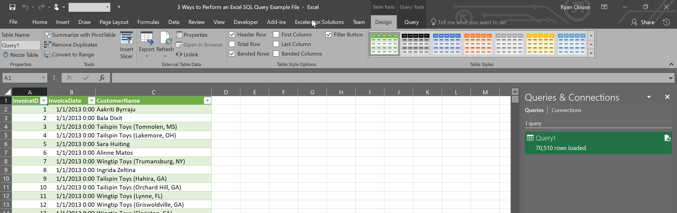
This will create a table on a new tab and you’ll also notice a new pane on the right titled “Connections & Queries”. It will display the name of your query (defaults to “Query1”, “Query2”, etc.) and you can rename the query by right-clicking and selecting “Rename”. You can also edit the query from this location as well. It will open up an interface with a sample of your data and you can add/remove columns, filter your data, or edit your source query from here.
Now that you’ve set up this Excel SQL query, you can simply refresh the data set with fresh data anytime by clicking “Refresh All” on the “Data” ribbon. A quick side note here. If you pivot this data, “Refresh All” will refresh pivot tables first and then the query. To update your pivot table, you’ll need to refresh all twice or update your pivot table manually. To me, one of the downsides of this approach is the results are always returned in a table. I personally do not like working with tables in Excel. That’s where using VBA for your SQL query can come in handy.
Excel SQL Query Using VBA
Using VBA to create your Excel SQL query is not as straight forward as the previous approach, but can still be an extremely useful method depending on your situation. I particularly like that the data is not returned to a table unless you designate it to be so. This technique will work on older versions of Microsoft Excel but will not work on Mac OSX versions of Excel since it uses and ADO connection.
To get started, open up the VBA editor by pressing alt+F11. Before beginning to write your code, you’ll need to ensure that the “Microsoft ActiveX Data Objects 2.0 Library” is referenced from the VBA Project. To do this, click on “Tools” in the ribbon menu at the top of the VBA editor. In the popup, ensure the library is checked as shown below. This allows the project to use the ADO connectors to create the connection to your database. Next, let’s dimension a few variables.

Dim Conn As New ADODB.Connection
Dim recset As New ADODB.Recordset
Dim sqlQry As String, sConnect As String
The Conn variable is will be used to represent the connection between our VBA project and the SQL database. The receset variable will represent a new record set through which we will give the command to perform our Excel SQL query using the connection we’ve established. Finally, the sqlQry variable will represent a string variable that is our SQL query command, and the sConnect variable will be a string representing the connection string the database requires. Let’s look at how to use these variables to perform a SQL query.
sqlQry = "select top 1000 si.InvoiceID, si.InvoiceDate, sc.CustomerName from Sales.Invoices si" & _
             " left join sales.Customers sc on sc.CustomerID = si.CustomerID"

sConnect = "Driver={SQL Server};Server=[Your Server Name Here]; Database=[Your Database Here];Trusted_Connection=yes;"

Conn.Open sConnect

Set recset = New ADODB.Recordset

    recset.Open sqlQry, Conn
    Sheet2.Cells(2, 1).CopyFromRecordset recset
    recset.Close

Conn.Close

Set recset = Nothing
While this may look complex, each step is relatively simple. Firstly, we set our sqlQry variable equal to a string that represents the syntax of our SQL query. We then create a connection string we can use in our next command to connect to the database. So, “Conn.Open” is the command to open the connection and “sConnect” is the string it uses to do so. “Trusted_Connection=yes” means that the connection will attempt to be established using your Microsoft credentials for the account you’re logged in as.
Now that the connection is open, we can open a new record set and pass it the sql command using the sqlQry variable, and tell it which connection to use by passing it the Conn variable. We can then use the VBA command “CopyFromRecordset” to paste the recordset anywhere in our workbook. It’s important to close both the record set and connection at this point. You also want to set your recset variable equal to nothing so it does not eat up valuable resources.
One of the downsides to using this method is that you must explicitly tell Excel some things that the previous approach did automatically. For example, this SQL query will not return any column headers. Therefore, you must explicitly tell Excel what to label your columns. Secondly, the data is not automatically cleared and the new query imported. You must also explicitly tell Excel to do this as well. Here is the final code with those commands added.
Sub SQL_Example()
Dim Conn As New ADODB.Connection
Dim recset As New ADODB.Recordset
Dim sqlQry As String, sConnect As String

Sheet2.Cells.ClearContents

sqlQry = "select top 1000 si.InvoiceID, si.InvoiceDate, sc.CustomerName from Sales.Invoices si" & _
            " left join sales.Customers sc on sc.CustomerID = si.CustomerID"

sConnect = "Driver={SQL Server};Server=[Your Server Name Here]; Database=[Your Database Name Here];Trusted_Connection=yes;"

Conn.Open sConnect
Set recset = New ADODB.Recordset

    recset.Open sqlQry, Conn
    Sheet2.Cells(2, 1).CopyFromRecordset recset
    recset.Close

Conn.Close
Set recset = Nothing

Sheet2.Cells(1, 1) = "Invoice ID"
Sheet2.Cells(1, 2) = "Invoice Date"
Sheet2.Cells(1, 3) = "Customer Name"

End Sub
My preference for using this approach is when I want the user to be able to pass parameters to my Excel SQL query. For example, I might have a dropdown of customer names the user could select. By using this tactic, I can easily add a dropdown of customer names the user can select, and pass that value to my SQL query in a where clause.
As you can see, both the built in Excel SQL query and the VBA method have pros and cons. I employ both in my everyday work depending on what situation I find myself in.
Excel SQL Query Using Microsoft Query
This option is likely the most complex option, but it has the added advantage of being compatible with some versions of Mac OSX. I won’t pretend to be an expert at creating Mac OSX compatible tools for Excel, but I have successfully used this implementation to create an embedded Excel SQL query for Macs in the past.
I also like this method because you can create popup style parameters. For example, you can prompt the user to input date range parameters at the time the SQL query is ran. Like the first example, running this query is as easy as clicking “Refresh All” on the Data ribbon. Let’s dive in to the details.
To get started here, click “Get Data” on the Data ribbon. In the menu that dropdowns select “From Other Sources” and, finally “From Microsoft Query”.

This will open a wizard for you to choose your data source. Double click “<New Data Source>” and you’ll be prompted to enter some information about your data source. Option 1 can be anything you wish that describes your data source. Option 2 should be “SQL Server”. Click “Connect” and it will pop up a third window where you can enter information about the server and login information. Be sure you select the “Options>>” dropdown so you can select the database you’re wanting to connect to.

You’ll now have a new data source in the original window. Double click the data source to bring up a table import wizard. If you want to import an entire table, you can do so here and even filter and sort the data using the import wizard. However, if you want to use your own custom query as we have been, just select any field and go through the wizard and import the data. When you come to screen that asks you if you want to return the data to Excel or edit in a query, return the data to Excel. It will then prompt you to select where you want the data returned in your workbook.
The query will return the data in a table format. To change it to your own custom SQL query, let’s follow these steps:
- Click anywhere in the data table.
- On the Excel Data Ribbon, in the “Queries & Connections” group, properties will no longer be grayed out like it normally is. Click this.
- In the popup – you’ll see another properties icon. Click this.
- In this popup, select the “Definition” tab and paste your SQL query in the “Command Text” input box.
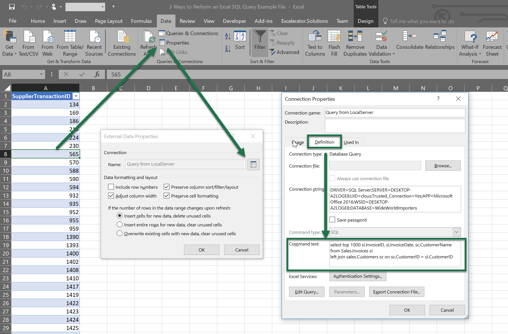
Now you’ve built an Excel SQL Query that can be refreshed anytime the workbook is refreshed. In my screengrab, the “Parameters” button is greyed out. If you want to add parameters to your query, you do so by adding “?” in your command text. That looks like this.
This creates a parameter the end user can interact with. You can have the user be prompted to enter an input when the workbook is refreshed, select a default value, or have it linked to a cell in the workbook. Even though this option is cumbersome to set up, I really enjoy using it. It allows me a lot of flexibility to have the user interact with the data. As I touched on in the beginning, I’ve had success using this option on Microsoft Office for Mac OSX. I don’t want to say this will work 100% of the time on a Mac because I’ve also had it fail. If anyone has any input on this, I’d love to hear from you.
Let me know your thoughts on these approaches in the comments! What other ways do you creatively get data into Excel from SQL data sources?
Cheers!
R