Queries in microsoft excel - Word и Excel - помощь в работе с программами

Create, load, or edit a query in Excel (Power Query)

Excel for Microsoft 365 Excel 2021 Excel 2019 Excel 2016 Excel 2013 Excel 2010 More…Less

Power Query offers several ways to create and load Power queries into your workbook. You can also set default query load settings in the Query Options window.

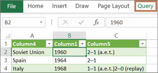
Tip To tell if data in a worksheet is shaped by Power Query, select a cell of data, and if the Query context ribbon tab appears, then the data was loaded from Power Query.

Know which environment you’re in Power Query is well-integrated into the Excel user interface, especially when you import data, work with connections, and edit Pivot Tables, Excel tables, and named ranges. To avoid confusion, it’s important to know which environment you are currently in, Excel or Power Query, at any point in time.

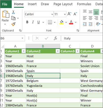
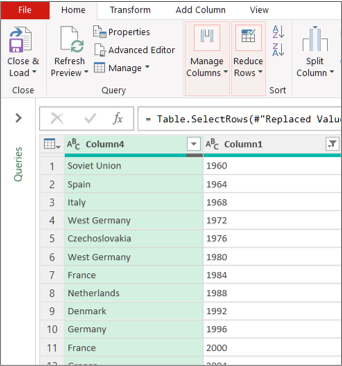
The familiar Excel worksheet , ribbon, and grid	The Power Query Editor ribbon and data preview

For example, manipulating data in an Excel worksheet is fundamentally different than Power Query. Furthermore, the connected data that you see in an Excel worksheet, may or may not have Power Query working behind the scenes to shape the data. This only occurs when you load the data to a worksheet or Data Model from Power Query.

Rename worksheet tabs It’s a good idea to rename worksheet tabs in a meaningful way, especially if you have a lot of them. It’s particularly important to clarify the difference between a worksheet of data, and a worksheet loaded from the Power Query Editor. Even if you have only two worksheets, one with an Excel table, called Sheet1, and the other a query created by importing that Excel table, called Table1, it’s easy to get confused. It’s always good practice to change the default names of worksheet tabs to names that make more sense to you. For example, rename Sheet1 to DataTable and Table1 to QueryTable. Now it’s clear which tab has the data and which tab has the query.

You can either create a query from imported data or create a blank query.

Create a query from imported data

This is the most common way to create a query.

Import some data. For more information, see Import data from external data sources.
Select a cell in the data and then select Query > Edit.

Create a blank query

You may want to just start from scratch. There are two ways to do this.

Select Data > Get Data > From Other Sources > Blank Query.
Select Data > Get Data > Launch Power Query Editor.

At this point, you can manually add steps and formulas if you know the Power Query M formula language well.

Or you can select Home and then select a command in the New Query group. Do one of the following.

Select New Source to add a data source. This command is just like the Data > Get Data command in the Excel ribbon.
Select Recent Sources to select from a data source you have been working with. This command is just like the Data > Recent Sources command in the Excel ribbon.
Select Enter Data to manually enter data. You might choose this command to try out the Power Query Editor independent of an external data source.

Assuming your query is valid and has no errors, you can load it back to a worksheet or Data Model.

Load a query from the Power Query Editor

In the Power Query Editor, do one of the following:

To load to a worksheet, select Home > Close & Load > Close & Load.
To load to a Data Model, select Home > Close & Load > Close & Load To.

In the Import Data dialog box, select Add this data to the Data Model.

Tip Sometimes the Load To command is dimmed or disabled. This can occur the first time you create a query in a workbook. If this occurs, select Close & Load, in the new worksheet, select Data > Queries & Connections > Queries tab, right click the query, and then select Load To. Alternatively, on the Power Query Editor ribbon select Query > Load To.

Load a query from the Queries and Connections pane

In Excel, you may want to load a query into another worksheet or Data Model.

In Excel, select Data > Queries & Connections, and then select the Queries tab.
In the list of queries, locate the query, right click the query, and then select Load To. The Import Data dialog box appears.
Decide how you want to import the data, and then select OK. For more information about using this dialog box, select the question mark (?).

There are several ways to edit a query loaded to a worksheet.

Edit a query from data in Excel worksheet

To edit a query, locate one previously loaded from the Power Query Editor, select a cell in the data, and then select Query > Edit.

Edit a query from the Queries & Connections pane

You may find the Queries & Connections pane is more convenient to use when you have many queries in one workbook and you want to quickly find one.

In Excel, select Data > Queries & Connections, and then select the Queries tab.
In the list of queries, locate the query, right click the query, and then select Edit.

Edit a query from the Query Properties dialog box

In Excel, select Data > Data & Connections > Queries tab, right click the query and select Properties, select the Definition tab in the Properties dialog box, and then select Edit Query.

Tip If you are in a worksheet with a query, select Data > Properties, select the Definition tab in the Properties dialog box, and then select Edit Query.

A Data Model typically contains several tables arranged in a relationship. You load a query to a Data Model by using the Load To command to display the Import Data dialog box, and then selecting the Add this data to the Data Model check box. For more information about Data Models, see Find out which data sources are used in a workbook data model, Create a Data Model in Excel, and Use multiple tables to create a PivotTable.

To open the Data Model, select Power Pivot > Manage.
At the bottom of the Power Pivot window, select the worksheet tab of the table you want.

Confirm that the correct table displays. A Data Model can have many tables.
Note the name of the table.
To close the Power Pivot window, select File > Close. It may take a few seconds to reclaim memory.
Select Data > Connections & Properties > Queries tab, right click the query, and then select Edit.
When finished making changes in the Power Query Editor, select File > Close & Load.

Result

The query in the worksheet and the table in the Data Model are updated.

If you notice that loading a query to a Data Model takes much longer than loading to a worksheet, check your Power Query steps to see if you are filtering a text column or a List structured column by using a Contains operator. This action causes Excel to enumerate again through the entire data set for each row. Furthermore, Excel can’t effectively use multithreaded execution. As a workaround, try using a different operator such as Equals or Begins With.

Microsoft is aware of this problem and it is under investigation.

You can load a Power Query:

To a worksheet. In the Power Query Editor, select Home > Close & Load > Close & Load.
To a Data Model. In the Power Query Editor, select Home > Close & Load > Close & Load To.

By default, Power Query loads queries to a new worksheet when loading a single query, and loads multiple queries at the same time to the Data Model. You can change the default behavior for all your workbooks or just the current workbook. When setting these options, Power Query doesn’t change query results in the worksheet or the Data Model data and annotations.

You can also dynamically override the default settings for a query by using the Import dialog box which displays after you select Close & Load To.

Global settings that apply to all your workbooks

In the Power Query Editor, select File > Options and settings > Query Options.
In the Query Options dialog box, on the left side, under the GLOBAL section, select Data Load.
Under the Default Query Load Settings section, do the following:
- Select Use standard load settings.
- Select Specify custom default load settings, and then select or clear Load to worksheet or Load to Data Model.

Tip At the bottom of the dialog box, you can select Restore Defaults to conveniently return to the default settings.

Workbook settings that only apply to the current workbook

In the Query Options dialog box, on the left side, under the CURRENT WORKBOOK section, select Data Load.
Do one or more of the following:
- Under Type Detection, select or clear Detect column types and headers for unstructured sources.
  
  The default behavior is to detect them. Clear this option if you prefer to shape the data yourself.
- Under Relationships, select or clear Create relationships between tables when adding to the Data Model for the first time.
  
  Before loading to the Data Model, the default behavior is to find existing relationships between tables, such as foreign keys in a relational database and import them with the data. Clear this option if you prefer to do this on your own.
- Under Relationships, select or clear Update relationships when refreshing queries loaded to the Data Model.
  
  The default behavior is to not update relationships. When refreshing queries already loaded to the Data Model, Power Query finds existing relationships between tables such as foreign keys in a relational database and updates them. This might remove relationships created manually after the data was imported or introduce new relationships. However, if you want to do this, select the option.
- Under Background Data, select or clear Allow data previews to download in the background.
  
  The default behavior is to download data previews in the background. Clear this option if you can want to see all the data right away.

What can I do with MS Query?

Using MS Query in Excel you can extract data from various sources such as:

Excel Files – you can extract data from External Excel files as well as run a SELECT query on your current Workbook
Access – you can extract data from Access Database files
MS SQL Server – you can extract data from Microsoft SQL Server Tables
CSV and Text – you can upload CSV or tabular Text files

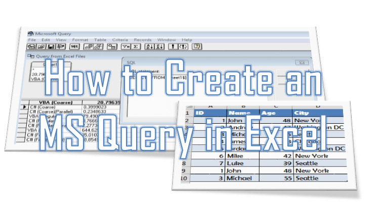
Step by Step – Microsoft Query in Excel

In this step by step tutorial I will show you how to create an Microsoft Query to extract data from either you current Workbook or an external Excel file.

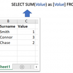
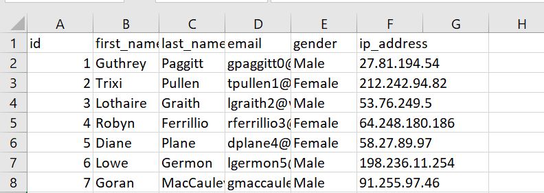
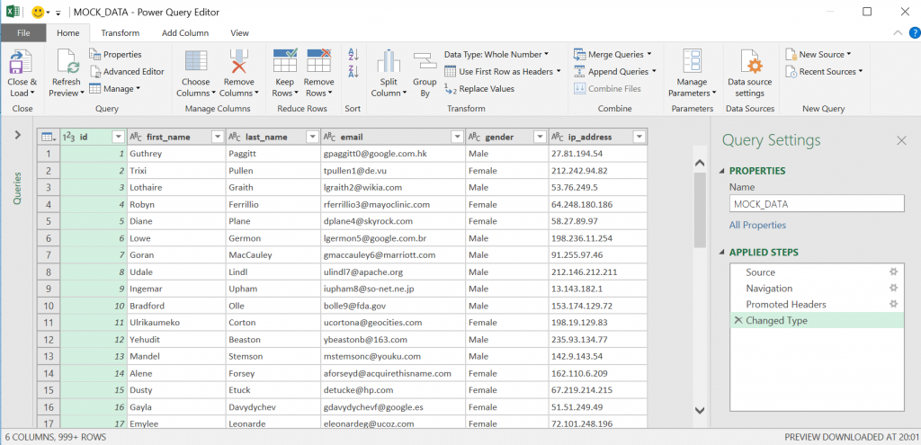
I will extract data from an External Excel file called MOCK DATA.xlsx. In this file I have a list of Male/Female mock-up customers. I will want to create a simple query to calculate how many are Male and how many Female.

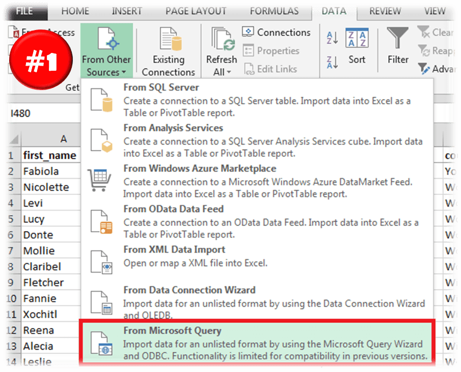
Open the MS Query (from Other Sources) wizard

Go to the DATA Ribbon Tab and click From Other Sources. Select the last option From Microsoft Query.

Select the Data Source

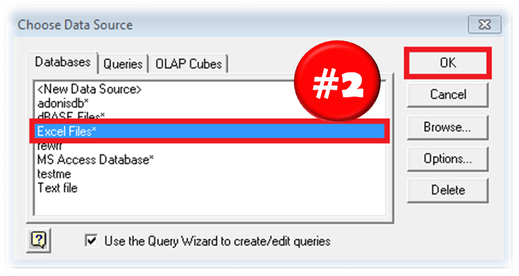Next we need to specify the Data Source for our Microsoft Query. Select Excel Files to proceed.

Select Excel Source File

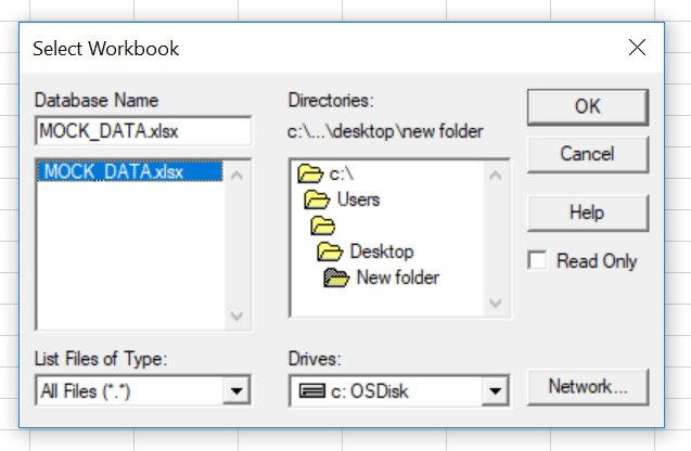Now we need to select the Excel file that will be the source for our Microsoft Query. In my example I will select my current Workbook, the same from which I am creating my MS Query.

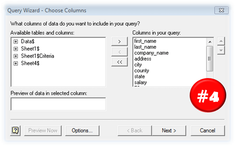
Select Columns for your MS Query

The Wizard now asks you to select Columns for your MS Query. If you plan to modify the MS Query manually later simply click OK. Otherwise select your Columns.

Return Query or Edit Query

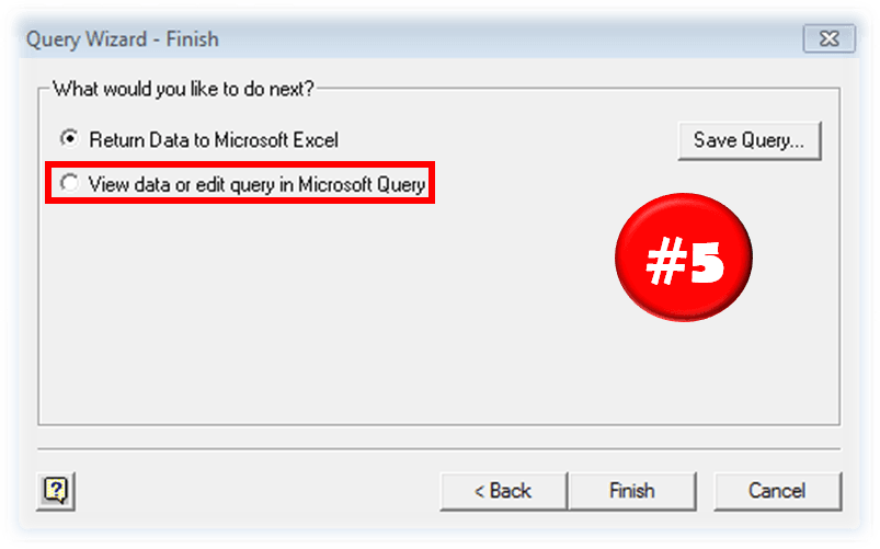Now you have two options:

Return Data to Microsoft Excel – this will return your query results to Excel and complete the Wizard
View data or edit query in Microsoft Query – this will open the Microsoft Query window and allow you to modify you Microsoft Query

Optional: Edit Query

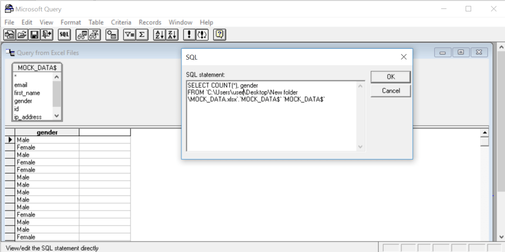If you select the View data or edit query in Microsoft Query option you can now open the SQL Edit Query window by hitting the SQL button. When you are done hit the return button (the one with the open door).

Import Data

When you are done modifying your SQL statement (as I in previous step). Click the Return data button in the Microsoft Query window.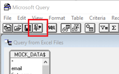
This should open the Import Data window which allows you to select when the data is to be dumped.
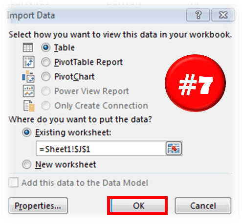Lastly, when you are done click OK on the Import Data window to complete running the query. You should see the result of the query as a new Excel table:

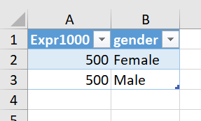
As in the window above I have calculated how many of the records in the original table where Male and how many Female.

AS you can see there are quite a lot of steps needed to achieve something potentially pretty simple. Hence there are a couple of alternatives thanks to the power of VBA Macro….

MS Query – Create with VBA

If you don’t want to use the SQL AddIn another way is to create these queries using a VBA Macro. Below is a quick macro that will allow you write your query in a simple VBA InputBox at the selected range in your worksheet.

Just use my VBA Code Snippet:

Sub ExecuteSQL()
    Attribute ExecuteSQL.VB_ProcData.VB_Invoke_Func = "Sn14"
    'AnalystCave.com
    On Error GoTo ErrorHandl
    Dim SQL As String, sConn As String, qt As QueryTable
    SQL = InputBox("Provide your SQL Query", "Run SQL Query")
    If SQL = vbNullString Then Exit Sub
    sConn = "OLEDB;Provider=Microsoft.ACE.OLEDB.12.0;;Password=;User ID=Admin;Data Source=" &amp; _
        ThisWorkbook.Path &amp; "/" &amp; ThisWorkbook.Name &amp; ";" &amp; _
        "Mode=Share Deny Write;Extended Properties=""Excel 12.0 Xml;HDR=YES"";"
    Set qt = ActiveCell.Worksheet.QueryTables.Add(Connection:=sConn, Destination:=ActiveCell)
    With qt
        .CommandType = xlCmdSql
        .CommandText = SQL
        .Name = Int((1000000000 - 1 + 1) * Rnd + 1)
        .RefreshStyle = xlOverwriteCells
        .Refresh BackgroundQuery:=False
    End With
    Exit Sub
ErrorHandl: MsgBox "Error: " &amp; Err.Description: Err.Clear
End Sub

Just create a New VBA Module and paste the code above. You can run it hitting the CTRL+SHIFT+S Keyboardshortcut or Add the Macro to your Quick Access Toolbar.

Learning SQL with Excel

Creating MS Queries is one thing, but you need to have a pretty good grasp of the SQL language to be able to use it’s true potential. I recommend using a simple Excel database (like Northwind) and practicing various queries with JOINs.

Alternatives in Excel – Power Query

Another way to run queries is to use Microsoft Power Query (also known in Excel 2016 and up as Get and Transform). The AddIn provided by Microsoft does require knowledge of the SQL Language, rather allowing you to click your way through the data you want to tranform.

MS Query vs Power Query Conclusions

MS Query Pros: Power Query is an awesome tool, however, it doesn’t entirely invalidate Microsoft Queries. What is more, sometimes using Microsoft Queries is quicker and more convenient and here is why:

Microsoft Queries are more efficient when you know SQL. While you can click your way through to Transform Data via Power Query someone who knows SQL will likely be much quicker in writing a suitable SELECT query
You can’t re-run Power Queries without the AddIn. While this obviously will be a less valid statement probably in a couple of years (in newer Excel versions), currently if you don’t have the AddIn you won’t be able to edit or re-run Queries created in Power Query

MS Query Cons: Microsoft Query falls short of the Power Query AddIn in some other aspects however:

Power Query has a more convenient user interface. While Power Queries are relatively easy to create, the MS Query Wizard is like a website from the 90’s
Power Query stacks operations on top of each other allowing more convenient changes. While an MS Query works or just doesn’t compile, the Power Query stacks each transform operation providing visibility into your Data Transformation task, and making it easier to add / remove operations

In short I encourage learning Power Query if you don’t feel comfortable around SQL. If you are advanced in SQL I think you will find using good ole Microsoft Queries more convenient. I would compare this to the Age-Old discussion between Command Line devs vs GUI devs…

Источник

Содержание

Создание SQL запроса в Excel
- Способ 1: использование надстройки
- Способ 2: использование встроенных инструментов Excel
- Способ 3: подключение к серверу SQL Server
Вопросы и ответы

SQL – популярный язык программирования, который применяется при работе с базами данных (БД). Хотя для операций с базами данных в пакете Microsoft Office имеется отдельное приложение — Access, но программа Excel тоже может работать с БД, делая SQL запросы. Давайте узнаем, как различными способами можно сформировать подобный запрос.

Читайте также: Как создать базу данных в Экселе

Язык запросов SQL отличается от аналогов тем, что с ним работают практически все современные системы управления БД. Поэтому вовсе не удивительно, что такой продвинутый табличный процессор, как Эксель, обладающий многими дополнительными функциями, тоже умеет работать с этим языком. Пользователи, владеющие языком SQL, используя Excel, могут упорядочить множество различных разрозненных табличных данных.

Способ 1: использование надстройки

Но для начала давайте рассмотрим вариант, когда из Экселя можно создать SQL запрос не с помощью стандартного инструментария, а воспользовавшись сторонней надстройкой. Одной из лучших надстроек, выполняющих эту задачу, является комплекс инструментов XLTools, который кроме указанной возможности, предоставляет массу других функций. Правда, нужно заметить, что бесплатный период пользования инструментом составляет всего 14 дней, а потом придется покупать лицензию.

Скачать надстройку XLTools

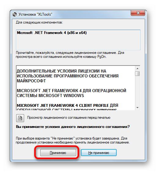
После того, как вы скачали файл надстройки xltools.exe, следует приступить к его установке. Для запуска инсталлятора нужно произвести двойной щелчок левой кнопки мыши по установочному файлу. После этого запустится окно, в котором нужно будет подтвердить согласие с лицензионным соглашением на использование продукции компании Microsoft — NET Framework 4. Для этого всего лишь нужно кликнуть по кнопке «Принимаю» внизу окошка.

После этого установщик производит загрузку обязательных файлов и начинает процесс их установки.

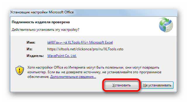
Далее откроется окно, в котором вы должны подтвердить свое согласие на установку этой надстройки. Для этого нужно щелкнуть по кнопке «Установить».

Затем начинается процедура установки непосредственно самой надстройки.

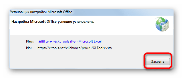
После её завершения откроется окно, в котором будет сообщаться, что инсталляция успешно выполнена. В указанном окне достаточно нажать на кнопку «Закрыть».

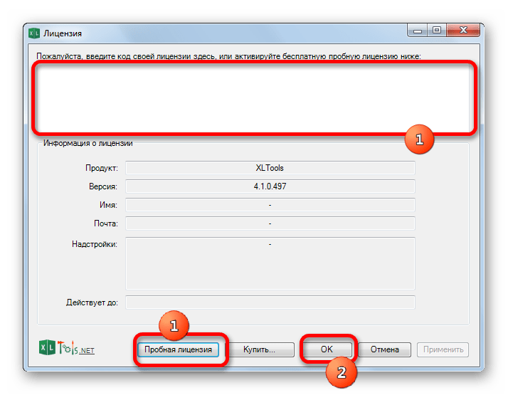
Надстройка установлена и теперь можно запускать файл Excel, в котором нужно организовать SQL запрос. Вместе с листом Эксель открывается окно для ввода кода лицензии XLTools. Если у вас имеется код, то нужно ввести его в соответствующее поле и нажать на кнопку «OK». Если вы желаете использовать бесплатную версию на 14 дней, то следует просто нажать на кнопку «Пробная лицензия».

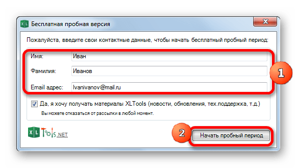
При выборе пробной лицензии открывается ещё одно небольшое окошко, где нужно указать своё имя и фамилию (можно псевдоним) и электронную почту. После этого жмите на кнопку «Начать пробный период».

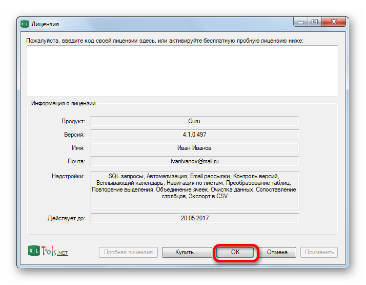
Далее мы возвращаемся к окну лицензии. Как видим, введенные вами значения уже отображаются. Теперь нужно просто нажать на кнопку «OK».

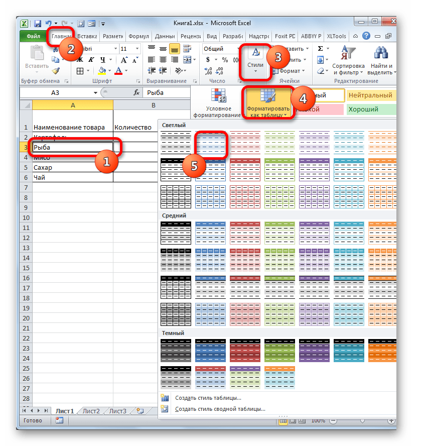
После того, как вы проделаете вышеуказанные манипуляции, в вашем экземпляре Эксель появится новая вкладка – «XLTools». Но не спешим переходить в неё. Прежде, чем создавать запрос, нужно преобразовать табличный массив, с которым мы будем работать, в так называемую, «умную» таблицу и присвоить ей имя.
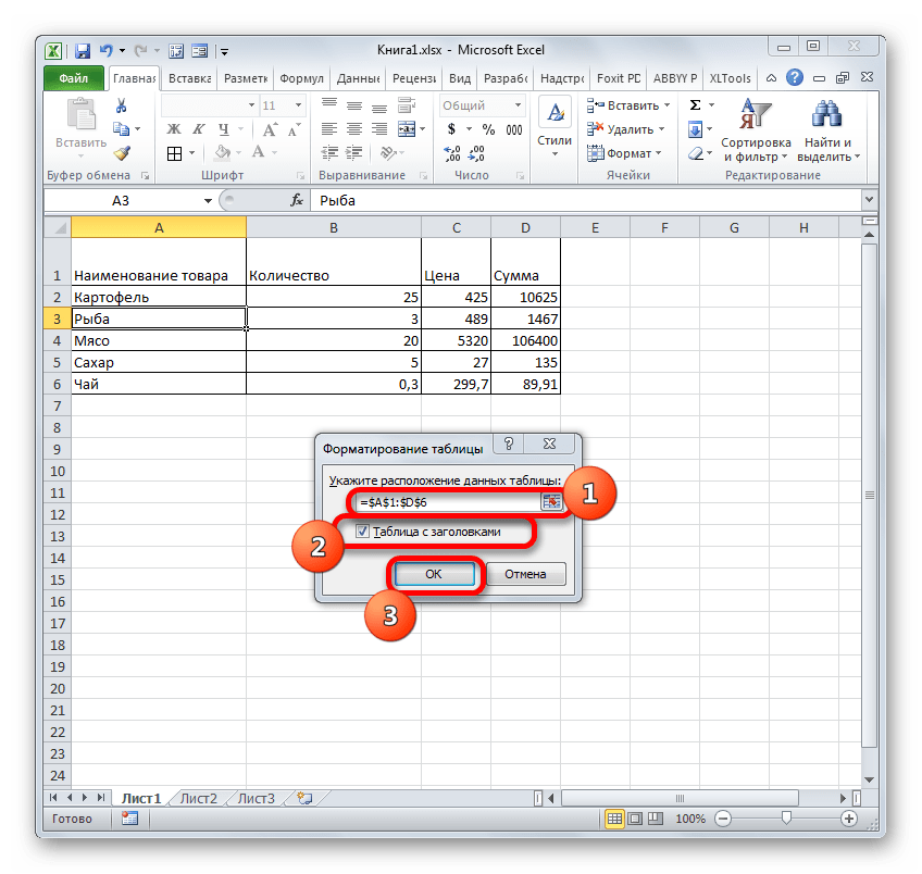
Для этого выделяем указанный массив или любой его элемент. Находясь во вкладке «Главная» щелкаем по значку «Форматировать как таблицу». Он размещен на ленте в блоке инструментов «Стили». После этого открывается список выбора различных стилей. Выбираем тот стиль, который вы считаете нужным. На функциональность таблицы указанный выбор никак не повлияет, так что основывайте свой выбор исключительно на основе предпочтений визуального отображения.

Вслед за этим запускается небольшое окошко. В нем указываются координаты таблицы. Как правило, программа сама «подхватывает» полный адрес массива, даже если вы выделили только одну ячейку в нем. Но на всякий случай не мешает проверить ту информацию, которая находится в поле «Укажите расположение данных таблицы». Также нужно обратить внимание, чтобы около пункта «Таблица с заголовками», стояла галочка, если заголовки в вашем массиве действительно присутствуют. Затем жмите на кнопку «OK».

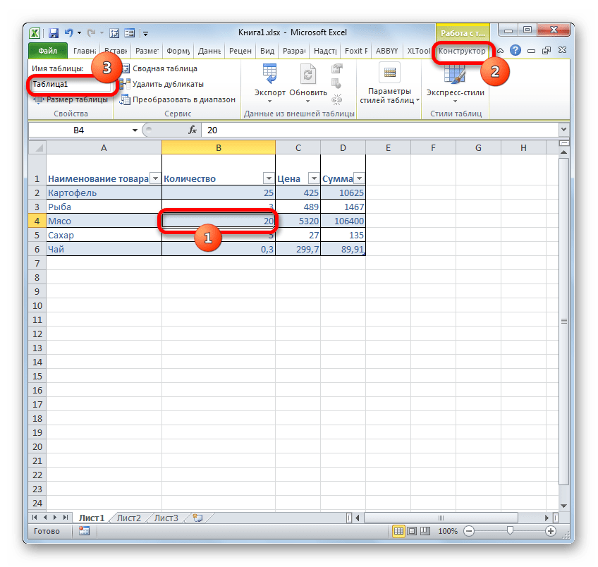
После этого весь указанный диапазон будет отформатирован, как таблица, что повлияет как на его свойства (например, растягивание), так и на визуальное отображение. Указанной таблице будет присвоено имя. Чтобы его узнать и по желанию изменить, клацаем по любому элементу массива. На ленте появляется дополнительная группа вкладок – «Работа с таблицами». Перемещаемся во вкладку «Конструктор», размещенную в ней. На ленте в блоке инструментов «Свойства» в поле «Имя таблицы» будет указано наименование массива, которое ему присвоила программа автоматически.

При желании это наименование пользователь может изменить на более информативное, просто вписав в поле с клавиатуры желаемый вариант и нажав на клавишу Enter.

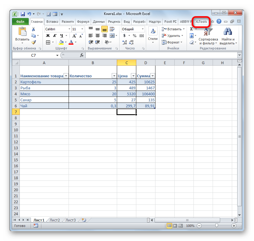
После этого таблица готова и можно переходить непосредственно к организации запроса. Перемещаемся во вкладку «XLTools».

После перехода на ленте в блоке инструментов «SQL запросы» щелкаем по значку «Выполнить SQL».

Запускается окно выполнения SQL запроса. В левой его области следует указать лист документа и таблицу на древе данных, к которой будет формироваться запрос.
В правой области окна, которая занимает его большую часть, располагается сам редактор SQL запросов. В нем нужно писать программный код. Наименования столбцов выбранной таблицы там уже будут отображаться автоматически. Выбор столбцов для обработки производится с помощью команды SELECT. Нужно оставить в перечне только те колонки, которые вы желаете, чтобы указанная команда обрабатывала.

Далее пишется текст команды, которую вы хотите применить к выбранным объектам. Команды составляются при помощи специальных операторов. Вот основные операторы SQL:
- ORDER BY – сортировка значений;
- JOIN – объединение таблиц;
- GROUP BY – группировка значений;
- SUM – суммирование значений;
- DISTINCT – удаление дубликатов.
Кроме того, в построении запроса можно использовать операторы MAX, MIN, AVG, COUNT, LEFT и др.

В нижней части окна следует указать, куда именно будет выводиться результат обработки. Это может быть новый лист книги (по умолчанию) или определенный диапазон на текущем листе. В последнем случае нужно переставить переключатель в соответствующую позицию и указать координаты этого диапазона.

После того, как запрос составлен и соответствующие настройки произведены, жмем на кнопку «Выполнить» в нижней части окна. После этого введенная операция будет произведена.

Урок: «Умные» таблицы в Экселе

Способ 2: использование встроенных инструментов Excel

Существует также способ создать SQL запрос к выбранному источнику данных с помощью встроенных инструментов Эксель.

Запускаем программу Excel. После этого перемещаемся во вкладку «Данные».

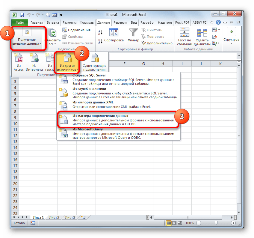
В блоке инструментов «Получение внешних данных», который расположен на ленте, жмем на значок «Из других источников». Открывается список дальнейших вариантов действий. Выбираем в нем пункт «Из мастера подключения данных».

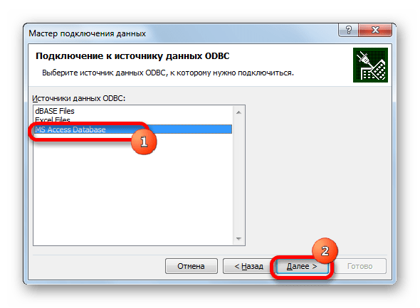
Запускается Мастер подключения данных. В перечне типов источников данных выбираем «ODBC DSN». После этого щелкаем по кнопке «Далее».

Открывается окно Мастера подключения данных, в котором нужно выбрать тип источника. Выбираем наименование «MS Access Database». Затем щелкаем по кнопке «Далее».

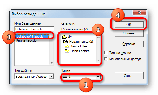
Открывается небольшое окошко навигации, в котором следует перейти в директорию расположения базы данных в формате mdb или accdb и выбрать нужный файл БД. Навигация между логическими дисками при этом производится в специальном поле «Диски». Между каталогами производится переход в центральной области окна под названием «Каталоги». В левой области окна отображаются файлы, расположенные в текущем каталоге, если они имеют расширение mdb или accdb. Именно в этой области нужно выбрать наименование файла, после чего кликнуть на кнопку «OK».

Вслед за этим запускается окно выбора таблицы в указанной базе данных. В центральной области следует выбрать наименование нужной таблицы (если их несколько), а потом нажать на кнопку «Далее».

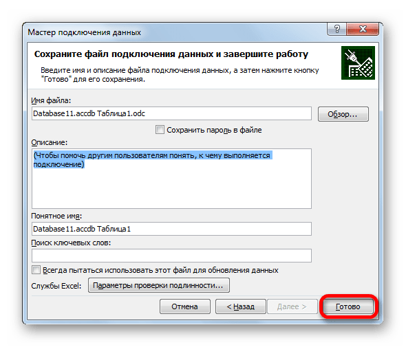
После этого открывается окно сохранения файла подключения данных. Тут указаны основные сведения о подключении, которое мы настроили. В данном окне достаточно нажать на кнопку «Готово».

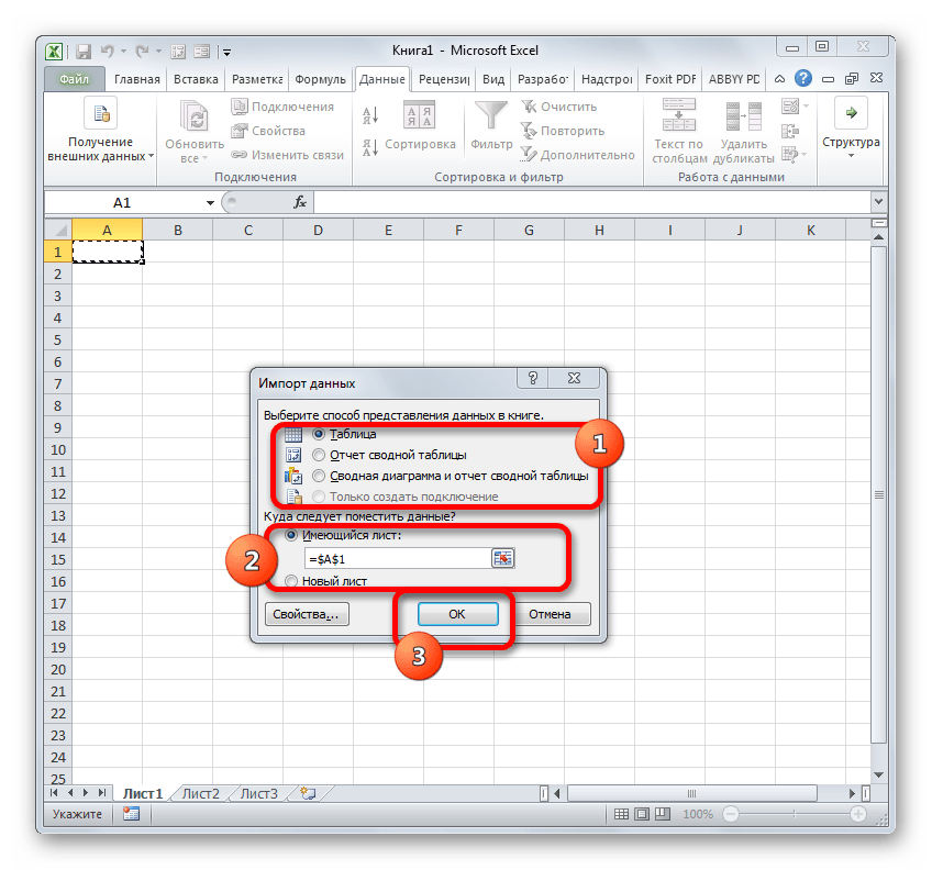
На листе Excel запускается окошко импорта данных. В нем можно указать, в каком именно виде вы хотите, чтобы данные были представлены:
- Таблица;
- Отчёт сводной таблицы;
- Сводная диаграмма.
Выбираем нужный вариант. Чуть ниже требуется указать, куда именно следует поместить данные: на новый лист или на текущем листе. В последнем случае предоставляется также возможность выбора координат размещения. По умолчанию данные размещаются на текущем листе. Левый верхний угол импортируемого объекта размещается в ячейке A1.

После того, как все настройки импорта указаны, жмем на кнопку «OK».

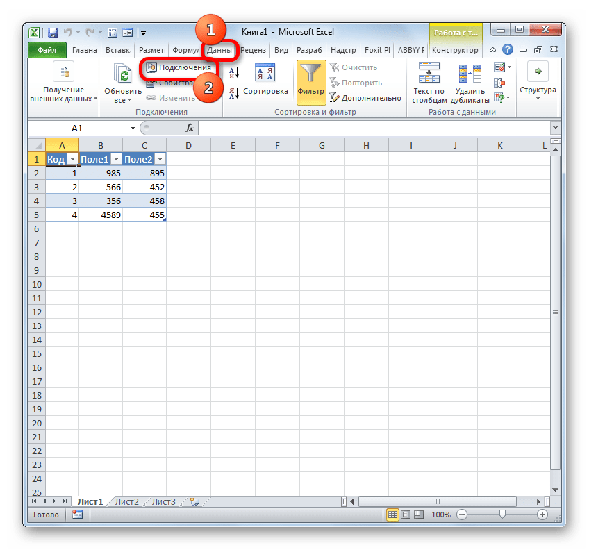
Как видим, таблица из базы данных перемещена на лист. Затем перемещаемся во вкладку «Данные» и щелкаем по кнопке «Подключения», которая размещена на ленте в блоке инструментов с одноименным названием.

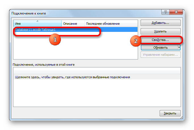
После этого запускается окно подключения к книге. В нем мы видим наименование ранее подключенной нами базы данных. Если подключенных БД несколько, то выбираем нужную и выделяем её. После этого щелкаем по кнопке «Свойства…» в правой части окна.

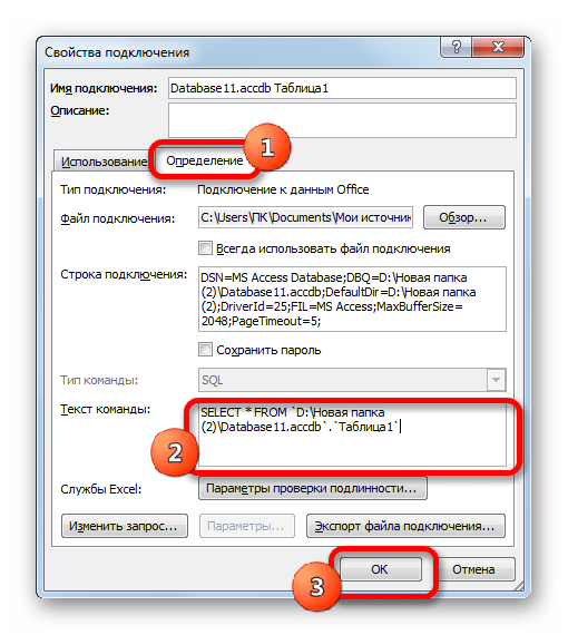
Запускается окно свойств подключения. Перемещаемся в нем во вкладку «Определение». В поле «Текст команды», находящееся внизу текущего окна, записываем SQL команду в соответствии с синтаксисом данного языка, о котором мы вкратце говорили при рассмотрении Способа 1. Затем жмем на кнопку «OK».

После этого производится автоматический возврат к окну подключения к книге. Нам остается только кликнуть по кнопке «Обновить» в нем. Происходит обращение к базе данных с запросом, после чего БД возвращает результаты его обработки назад на лист Excel, в ранее перенесенную нами таблицу.

Способ 3: подключение к серверу SQL Server

Кроме того, посредством инструментов Excel существует возможность соединения с сервером SQL Server и посыла к нему запросов. Построение запроса не отличается от предыдущего варианта, но прежде всего, нужно установить само подключение. Посмотрим, как это сделать.

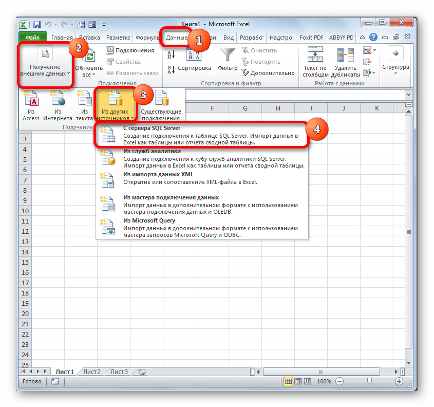
Запускаем программу Excel и переходим во вкладку «Данные». После этого щелкаем по кнопке «Из других источников», которая размещается на ленте в блоке инструментов «Получение внешних данных». На этот раз из раскрывшегося списка выбираем вариант «С сервера SQL Server».

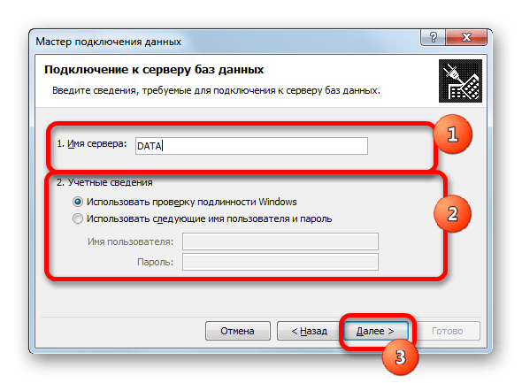
Происходит открытие окна подключения к серверу баз данных. В поле «Имя сервера» указываем наименование того сервера, к которому выполняем подключение. В группе параметров «Учетные сведения» нужно определиться, как именно будет происходить подключение: с использованием проверки подлинности Windows или путем введения имени пользователя и пароля. Выставляем переключатель согласно принятому решению. Если вы выбрали второй вариант, то кроме того в соответствующие поля придется ввести имя пользователя и пароль. После того, как все настройки проведены, жмем на кнопку «Далее». После выполнения этого действия происходит подключение к указанному серверу. Дальнейшие действия по организации запроса к базе данных аналогичны тем, которые мы описывали в предыдущем способе.

Как видим, в Экселе SQL запрос можно организовать, как встроенными инструментами программы, так и при помощи сторонних надстроек. Каждый пользователь может выбрать тот вариант, который удобнее для него и является более подходящим для решения конкретно поставленной задачи. Хотя, возможности надстройки XLTools, в целом, все-таки несколько более продвинутые, чем у встроенных инструментов Excel. Главный же недостаток XLTools заключается в том, что срок бесплатного пользования надстройкой ограничен всего двумя календарными неделями.

Еще статьи по данной теме:

Помогла ли Вам статья?

Источник

26 Sep ’22 by Antonio Nakić-Alfirević

SQL Query function in Excel

If you’re reading this article you probably know that Google Sheets has a QUERY function that allows you to run SQL-like queries against data in the sheet. This function lets you do all sorts of gymnastics with the data in your sheet, be it filtering, aggregating, or pivoting data.

Being a fully-fledged desktop app, Excel tends to be more feature-rich than Google Sheets. This is especially true in the data analytics department where Excel shines with advanced Excel functions as well as Power Query functionality.

However, Excel doesn’t natively have a QUERY function that you can use in cells on the sheet.

In this blog post, I’m going to show you how to add a QUERY function to Excel and give a few examples of how to use it.

First look

Let’s start by taking a look at the function in action.

Simple SELECT query examples

The function is pretty straightforward. It accepts the SQL query as the first parameter and returns a table with the results of the query.

The results automatically spill to the necessary amount of space. This spilling behavior relies on the dynamic array functionality that’s available in Excel 365 (but isn’t in earlier versions of Microsoft Excel).

Works with Excel tables

In Google Sheets, the QUERY function references data by address (e.g. “A1:B10”) while columns are referenced by letters (e.g. A, B, C…).

This works but has some drawbacks:

It makes the query sensitive to the location of the data. If the data is moved or if columns are reordered, the query will break.
It makes the query difficult to read since it uses range addresses and column letters instead of table and column names (e.g. Employees, DateOfBirth…)
Adding or removing rows can break the query. For example, if the provided range is “A1:H10” the query will only take into account the first 10 rows. If additional rows are added, the query will not take them into account. You can get around this by omitting the end row number (e.g. “A1:H”), but this means that there must be no other content below the data range.

Excel, on the other hand, allows explicitly defining tables (aka ListObjects) that delineate the areas that hold data. Each Excel table has a name, as do its columns. This makes Excel tables very similar to database tables and makes them easier to work with from SQL.

Explicitly defined tables in Excel

Full SQL syntax support (SQLite)

Under the hood, the Windy.Query function is powered by SQLite – a small but powerful embedded database engine.

When called, the function passes the query to the built-in SQLite engine which has an adapter that lets it use Excel tables as its data source.

This means that the entire SQLite syntax is available for use in queries. In comparison, in Google Sheets, the query syntax is rather limited. It only supports a single table (no joins) and a very small set of built-in functions.

Examples of use

Since the engine under the hood is SQLite, queries can use all operations available in SQLite, including table joins, temp tables, column table expressions, window functions etc… Let’s go over some examples of how to use these in Excel.

Joining tables

Here’s an example of a simple one-to-many join:

Simple one-to-many SQL join

The usual way of doing a simple operation such as this one in Excel would be to use xlookup or PowerQuery, but SQL is now another option. And if we needed anything more complex than a simple join, SQL would quickly shine as the most powerful and convenient option of the three.

Merging table rows (union)

Another way we might want to combine two (or more) tables is to combine their rows. We can do this with a SQL UNION operator.

The tables might have some rows in common. If we want to keep only one instance of such rows we would use the regular UNION operator. If we want to keep both versions of rows that are in common, we would use the UNION ALL operator.

Merging rows from two tables

Finding differences between two tables

In the previous example, we had two tables that had some rows in common and some rows not. Let’s assume, for example, that the first table contains last year’s list of employees and the second table is the new list of employees.

If we wanted to find out the differences between the two tables, we could easily do that with a bit of SQL.

All of the rows that are in the first table but not in the second one we will mark as “deleted”. All of the rows that are in the second table but not in the first one we will mark as “added”. Here’s what that SQL query looks like:

select
	id, name, 'deleted'
from
	employees e where not exists (select * from Employees_New en where e.id == en.Id)
union
select
	id, name, 'added'
from
	employees_new en where not exists (select * from Employees e where e.id == en.Id)

And here’s what the result looks like:

Calculating a diff between two tables

Ranking rows

Another useful thing we might want to do is rank rows based on some criteria. For example, suppose we have a table with a list of cities. For each city we have its population and the country it belongs to.

Our task is to find the top 3 cities in each country based on population. Here’s how we might do that in SQL.

-- we use this CTE so we can reference the calculated 'rank_pop' column in the where clause
with cte as (
	select
		city,
		country,
		population,
		-- using the RANK() window function
		RANK() OVER (PARTITION BY country ORDER BY population) as rank_pop
	from
		cities c)
select
	*
from
	cte
where
	-- filtering by the 'rank_pop' column from the CTE
	rank_pop <= 3
order by country, rank_pop

Rank cities by population in each country, return top 3 for each country

This query is a bit more complex than the previous ones. It uses a common table expression and a window function (the rank function), and showcases the ability to write complex SQL in queries.

Queries can also make use of dozens of built-in SQLite functions. Various specialized extended functions such as RegexReplace, GPSDist (GPS distance between two points) and LevDist (fuzzy text matching) are also available.

Updating tables

OK, this next example is a bit of a hack, but a useful one… The query you supply doesn’t need to be a SELECT query. You can do UPDATE/INSERT/DELETE statements as well, and these will modify the data in the target Excel tables.

Updating workbook tables with SQL

This can be a handy way to clean and transform data in your tables in place, without having to export/import the data to an external database (e.g. SQL Server, MySql, Postgres…).

This works because the SQLite engine isn’t copying the data. Rather, it’s using an adapter that lets it access live data in the Excel table.

How does the function see Excel tables?

At first glance, it might seem strange that the query can access your workbook tables. After all, we did not pass them in as parameters, and functions normally only work with parameters that are passed to them.

However, the Windy.Query function is aware of the workbook it’s being called from and it can read data from the workbook’s tables without the need for passing them in as parameters. This makes the function much easier to call especially when working with multiple tables.

Column Headers

Results returned by the Windy.Query function can optionally include headers. This is controlled by the second parameter of the function.

Toggling column headers on/off

The texts in the column headers are determined by the SQL query itself. You can easily rename result columns by aliasing them in the select list.

Aliasing column headers

Automatically refresh results

By default, the SQL query runs as a one-off operation when you enter the formula but does not refresh if the source tables change. However, if you want the query to refresh whenever one of the source tables changes, you can easily do so by setting the autoRefresh argument to true.

Automatic refresh of results when source data changes

Note that the auto-refresh functionality relies on Excel’s RTD (Real-Time Data) server. The RTD server usually throttles updates so functions don’t overwhelm Excel with frequent updates. The default throttle interval is 2s meaning that the function will not update more than once every 2s. To improve responsiveness, you can lower this value to something like 20ms. The simplest way to do this is through the “Configure” dialog in the QueryStorm runtime’s ribbon.

Adjusting the RTD interval in Excel

Passing parameters

When needed, SQL queries can use values from cells as parameters. To use a cell as a parameter in a query, start by giving the cell a name (named range).

Give the parameter cell a name

Once the cell has a name, you can reference it in the query using the @paramName or $paramName syntax.

Use the parameter in the SQL query

If automatic refresh is turned on, results will automatically refresh whenever one of the parameter cells changes its value.

Automatic refresh of results when parameter cell changes

Performance

This is all well and good for small tables, you might think, but how does it handle large data sets? Well, it handles them quite well. The function can read source tables of 100k rows and 10 columns within a few milliseconds and can return this amount of data in a second or two. In addition to this, all columns are automatically indexed so searches and joins are extremely performant as well.

This makes the function perform very well, both from the data throughput standpoint as well as from the computational one.

OK, so is this better than the Google Sheets version of the QUERY function?

Yes, dah. Did you read the previous chapters? 😛

Installing the Windy.Query function

So how do you install this function into your Excel? It’s a simple 2-step process.

Step 1 is to install the QueryStorm Runtime add-in (if you don’t already have it). This is a free, 4MB add-in for Excel that lets you install and use various extensions for Excel. It’s basically an app store for Excel.

Step 2 is to click the “Extensions” button in the “QueryStorm” tab in the Excel ribbon, find the Windy.Query package in the “Online” tab, and install it.

What happens if I share the workbook with a user who doesn’t have the function?

Nothing bad. If the other user doesn’t have the function installed, they will see the last results of the query that were returned on your machine. They just won’t be able to refresh the results.

Advanced SQL query editor

Writing SQL queries in the formula bar can get a bit unwieldy. To make queries easier to write, it’s better to use a proper editor, preferably one that offers syntax highlighting and code completion for SQL and knows about the tables in your workbook.

For this purpose, I recommend using the QueryStorm IDE. This is an advanced IDE that lets you use SQL in Excel. You can write the query in the QueryStorm code editor and then paste the query into the Windy.Query function when you’re happy with it (if needed).

Using the QueryStorm IDE to write SQL queries in Excel

The IDE does more than just allow using SQL in Excel. You can use it to create and share functions and addins for Excel. In fact the QueryStorm IDE was used to create the Windy.Query function itself.

The IDE has a free community version for individuals and small companies, while users in larger companies can make use of the free trial license. For paid licenses, check out the pricing page.

You can read more in this blog post that’s dedicated to the QueryStorm SQL IDE.

Video demonstration

For a video demonstration of the Windy.Query function, take a look the following video:

Источник

See Also

Need more help?

Want more options?

What can I do with MS Query?

Step by Step – Microsoft Query in Excel

Open the MS Query (from Other Sources) wizard

Select the Data Source

Select Excel Source File

Select Columns for your MS Query

Return Query or Edit Query

Optional: Edit Query

Import Data

MS Query – Create with VBA

Learning SQL with Excel

Alternatives in Excel – Power Query

MS Query vs Power Query Conclusions

Способ 1: использование надстройки

Способ 2: использование встроенных инструментов Excel

Способ 3: подключение к серверу SQL Server

Еще статьи по данной теме:

Помогла ли Вам статья?

26 Sep ’22 by Antonio Nakić-Alfirević

SQL Query function in Excel

First look

Works with Excel tables

Full SQL syntax support (SQLite)

Examples of use

Joining tables

Merging table rows (union)

Finding differences between two tables

Ranking rows

Updating tables

How does the function see Excel tables?

Column Headers

Automatically refresh results

Passing parameters

Performance

OK, so is this better than the Google Sheets version of the QUERY function?

Installing the Windy.Query function

What happens if I share the workbook with a user who doesn’t have the function?

Advanced SQL query editor

Video demonstration