
If data is always on a journey, then Excel is like Grand Central Station. Imagine that data is a train filled with passengers that regularly enters Excel, makes changes, and then leaves. There are dozens of ways to enter Excel, which imports data of all types and the list keeps growing. Once data is in Excel, it’s ready to change shape just the way you want using Power Query. Data, like all of us, also requires «care and feeding» to keep things running smoothly. That’s where connection, query, and data properties come in. Finally, data leaves the Excel train station in many ways: imported by other data sources, shared as reports, charts, and PivotTables, and exported to Power BI and Power Apps.
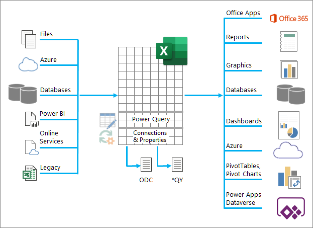
Here are the main things you can do while data is in the Excel train station:
-
Import You can import data from many different external data sources. These data sources can be on your machine, in the cloud, or half-way around the world. For more information, see Import data from external data sources.
-
Power Query You can use Power Query (previously called Get & Transform) to create queries to shape, transform, and combine data in a variety of ways. You can export your work as a Power Query Template to define a data flow operation in Power Apps. You can even create a data type to supplement linked data types. For more information, see Power Query for Excel Help.
-
Security Data privacy, credentials, and authentication are always an ongoing concern. For more information, see Manage data source settings and permissions and Set privacy levels.
-
Refresh Imported data usually requires a refresh operation to bring in changes, such as additions, updates, and deletes, to Excel. For more information, see Refresh an external data connection in Excel.
-
Connections/Properties Each external data source has assorted connection and property information associated with it that sometimes requires changes depending on your circumstances. For more information, see Manage external data ranges and their properties, Create, edit, and manage connections to external data, and Connection properties.
-
Legacy Traditional methods, such as Legacy Import Wizards and MSQuery, are still available for use. For more information, see Data import and analysis options and Use Microsoft Query to retrieve external data.
The following sections provide more details of what’s going on behind the scenes at this busy, Excel train station.
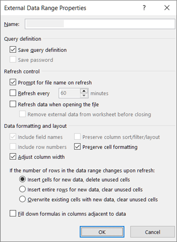
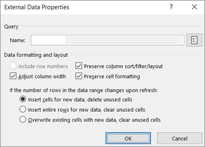
There are connection, query, and external data range properties. Connection and query properties both contain traditional connection information. In a dialog box title, Connection Properties means there is no query associated with it, but Query Properties means there is. External data range properties control the layout and format of data. All data sources have an External Data Properties dialog box, but data sources that have associated credential and refresh information use the larger External Range Data Properties dialog box.
The following information summarizes the most important dialog boxes, panes, command paths, and corresponding help topics.
|
Dialog Box or Pane |
Tabs and tunnels |
Main Help topic |
|---|---|---|
|
Recent sources Data > Recent Sources |
(No tabs) Tunnels to Connect > Navigator dialog box |
Manage data source settings and permissions |
|
Connection Properties Data > Queries & Connections > Connections tab > (right click a connection) > Properties |
Usage tab |
Connection properties |
|
Query Properties
Data > Existing Connections > (right click a connection) > Edit Connection Properties |
Usage tab |
Connection properties |
|
Queries & Connections Data > Queries & Connections |
Queries tab |
Connection properties |
|
Existing Connections Data > Existing Connections |
Connections tab |
Connect to external data |
|
External data properties |
Used in tab (from Connection Properties dialog box) Refresh button on the right tunnels to Query Properties |
Manage external data ranges and their properties |
|
Connection Properties > Definition tab > Export Connection File |
(No tabs) Tunnels to |
Create, edit, and manage connections to external data |
Data in an Excel workbook can come from two different locations. The data may be stored directly in the workbook, or it may be stored in an external data source, such as a text file, a database, or an Online Analytical Processing (OLAP) cube. This external data source is connected to the workbook through a data connection, which is a set of information that describes how to locate, log in to, and access the external data source.
The main benefit of connecting to external data is that you can periodically analyze this data without repeatedly copying the data to your workbook, which is an operation that can be time consuming and prone to error. After connecting to external data, you can also automatically refresh (or update) your Excel workbooks from the original data source whenever the data source is updated with new information.
Connection information is stored in the workbook and can also be stored in a connection file, such as an Office Data Connection (ODC) file (.odc) or a Data Source Name file (.dsn).
To bring external data into Excel, you need access to the data. If the external data source that you want to access is not on your local computer, you may need to contact the administrator of the database for a password, user permissions, or other connection information. If the data source is a database, make sure that the database is not opened in exclusive mode. If the data source is a text file or a spreadsheet, make sure that another user does not have it open for exclusive access.
Many data sources also require an ODBC driver or OLE DB provider to coordinate the flow of data between Excel, the connection file, and the data source.
The following diagram summarizes the key points about data connections.
1. There are a variety of data sources that you can connect to: Analysis Services, SQL Server, Microsoft Access, other OLAP and relational databases, spreadsheets, and text files.
2. Many data sources have an associated ODBC driver or OLE DB provider.
3. A connection file defines all the information that is needed to access and retrieve data from a data source.
4. Connection information is copied from a connection file into a workbook, and the connection information can easily be edited.
5. The data is copied into a workbook so that you can use it just as you use data stored directly in the workbook.
To find connection files, use the Existing Connections dialog box. (Select Data > Existing Connections.) Using this dialog box, you can see the following types of connections:
-
Connections in the workbook
This list displays all the current connections in the workbook. The list is created from connections that you already defined, that you created by using the Select Data Source dialog box of the Data Connection Wizard, or from connections that you previously selected as a connection from this dialog box.
-
Connection files on your computer
This list is created from the My Data Sources folder that is usually stored in the Documents folder.
-
Connection files on the network
This list can be created from a set of folders on your local network, the location of which can be deployed across the network as part of the deployment of Microsoft Office group policies, or a SharePoint library.
You can also use Excel as a connection file editor to create and edit connections to external data sources that are stored in a workbook or in a connection file. If you don’t find the connection that you want, you can create a connection by clicking Browse for More to display the Select Data Source dialog box, and then clicking New Source to start the Data Connection Wizard.
After you create the connection, you can use the Connection Properties dialog box (Select Data > Queries & Connections > Connections tab > (right click a connection) > Properties) to control various settings for connections to external data sources, and to use, reuse, or switch connection files.
Note Sometimes, the Connection Properties dialog box is named the Query Properties dialog box when there is a query created in Power Query (formerly called Get & Transform) associated with it.
If you use a connection file to connect to a data source, Excel copies the connection information from the connection file into the Excel workbook. When you make changes by using the Connection Properties dialog box, you are editing the data connection information that is stored in the current Excel workbook and not the original data connection file that may have been used to create the connection (indicated by the file name that is displayed in the Connection File property on the Definition tab). After you edit the connection information (with the exception of the Connection Name and Connection Description properties), the link to the connection file is removed and the Connection File property is cleared.
To ensure that the connection file is always used when a data source is refreshed, click Always attempt to use this file to refresh this data on the Definition tab. Selecting this check box ensures that updates to the connection file will always be used by all workbooks that use that connection file, which must also have this property set.
By using the Connections dialog box, you can easily manage these connections, including creating, editing, and deleting them (Select Data > Queries & Connections > Connections tab > (right click a connection) > Properties.) You can use this dialog box to do the following:
-
Create, edit, refresh, and delete connections that are in use in the workbook.
-
Verify the source of external data. You may want to do this in case the connection was defined by another user.
-
Show where each connection is used in the current workbook.
-
Diagnose an error message about connections to external data.
-
Redirect a connection to a different server or data source, or replace the connection file for an existing connection.
-
Make it easy to create and share connection files with users.
Connection files are particularly useful for sharing connections on a consistent basis, making connections more discoverable, helping to improve security of connections, and facilitating data source administration. The best way to share connection files is to put them in a secure and trusted location, such as a network folder or SharePoint library, where users can read the file but only designated users can modify the file. For more information, see Share data with ODC.
Using ODC files
You can create Office Data Connection (ODC) files (.odc) by connecting to external data through the Select Data Source dialog box or by using the Data Connection Wizard to connect to new data sources. An ODC file uses custom HTML and XML tags to store the connection information. You can easily view or edit the contents of the file in Excel.
You can share connection files with other people to give them the same access that you have to an external data source. Other users don’t need to set up a data source to open the connection file, but they may need to install the ODBC driver or OLE DB provider required to access the external data on their computer.
ODC files are the recommended method for connecting to data and sharing data. You can easily convert other traditional connection files (DSN, UDL, and query files) to an ODC file by opening the connection file and then clicking the Export Connection File button on the Definition tab of the Connection Properties dialog box.
Using query files
Query files are text files that contain data source information, including the name of the server where the data is located and the connection information that you provide when you create a data source. Query files are a traditional way for sharing queries with other Excel users.
Using .dqy query files You can use Microsoft Query to save .dqy files that contain queries for data from relational databases or text files. When you open these files in Microsoft Query, you can view the data returned by the query and modify the query to retrieve different results. You can save a .dqy file for any query that you create, either by using the Query Wizard or directly in Microsoft Query.
Using .oqy query files You can save .oqy files to connect to data in an OLAP database, either on a server or in an offline cube file (.cub). When you use the Multi-Dimensional Connection Wizard in Microsoft Query to create a data source for an OLAP database or cube, an .oqy file is created automatically. Because OLAP databases aren’t organized in records or tables, you can’t create queries or .dqy files to access these databases.
Using .rqy query files Excel can open query files in .rqy format to support OLE DB data source drivers that use this format. For more information, see the documentation for your driver.
Using .qry query files Microsoft Query can open and save query files in .qry format for use with earlier versions of Microsoft Query that cannot open .dqy files. If you have a query file in .qry format that you want to use in Excel, open the file in Microsoft Query, and then save it as a .dqy file. For information about saving .dqy files, see Microsoft Query Help.
Using .iqy Web query files Excel can open .iqy Web query files to retrieve data from the Web. For more information, see Export to Excel from SharePoint.
An external data range (also called a query table) is a defined name or table name that defines the location of the data brought into a worksheet. When you connect to external data, Excel automatically creates an external data range. The only exception to this is a PivotTable report connected to a data source, which does not create an external data range. In Excel, you can format and lay out an external data range or use it in calculations, as with any other data.
Excel automatically names an external data range as follows:
-
External data ranges from Office Data Connection (ODC) files are given the same name as the file name.
-
External data ranges from databases are named with the name of the query. By default Query_from_source is the name of the data source that you used to create the query.
-
External data ranges from text files are named with the text file name.
-
External data ranges from Web queries are named with the name of the Web page from which the data was retrieved.
If your worksheet has more than one external data range from the same source, the ranges are numbered. For example, MyText, MyText_1, MyText_2, and so on.
An external data range has additional properties (not to be confused with connection properties) that you can use to control the data, such as the preservation of cell formatting and column width. You can change these external data range properties by clicking Properties in the Connections group on the Data tab, and then making your changes in the External Data Range Properties or External Data Properties dialog boxes.
|
|
|
There are several data objects (such as an external data range and PivotTable report) that you can use to connect to different data sources. However, the type of data source that you can connect to is different between each data object.
You can use and refresh connected data in Excel Services. As with any external data source, you may need to authenticate your access. For more information, see Refresh an external data connection in Excel. For more information about credentials, see Excel Services Authentication Settings.
The following table summarizes which data sources are supported for each data object in Excel.
|
Excel |
Creates |
OLE |
ODBC |
Text |
HTML |
XML |
SharePoint |
|
|
Import Text Wizard |
Yes |
No |
No |
Yes |
No |
No |
No |
|
|
PivotTable report |
No |
Yes |
Yes |
Yes |
No |
No |
Yes |
|
|
PivotTable report |
No |
Yes |
No |
No |
No |
No |
No |
|
|
Excel Table |
Yes |
Yes |
Yes |
No |
No |
Yes |
Yes |
|
|
XML Map |
Yes |
No |
No |
No |
No |
Yes |
No |
|
|
Web Query |
Yes |
No |
No |
No |
Yes |
Yes |
No |
|
|
Data Connection Wizard |
Yes |
Yes |
Yes |
Yes |
Yes |
Yes |
Yes |
|
|
Microsoft Query |
Yes |
No |
Yes |
Yes |
No |
No |
No |
|
Note: These files, a text file imported by using the Import Text Wizard, an XML file imported by using an XML Map, and an HTML or XML file imported by using a Web Query, do not use an ODBC driver or OLE DB provider to make the connection to the data source.
Excel Services workaround for Excel tables and named ranges
If you want to display an Excel workbook in Excel Services, you can connect to and refresh data, but you must use a PivotTable report. Excel Services does not support external data ranges, which means that Excel Services does not support an Excel Table connected to a data source, a Web query, an XML map, or Microsoft Query.
However, you can work around this limitation by using a PivotTable to connect to the data source, and then design and layout the PivotTable as a two-dimensional table without levels, groups, or subtotals so that all desired row and column values are displayed.
Let’s take a trip down database memory lane.
About MDAC, OLE DB, and OBC
First of all, apologies for all the acronyms. Microsoft Data Access Components (MDAC) 2.8 is included with Microsoft Windows . With MDAC, you can connect to and use data from a wide variety of relational and nonrelational data sources. You can connect to many different data sources by using Open Database Connectivity (ODBC) drivers or OLE DB providers, which are either built and shipped by Microsoft or developed by various third parties. When you install Microsoft Office, additional ODBC drivers and OLE DB providers are added to your computer.
To see a complete list of OLE DB providers installed on your computer, display the Data Link Properties dialog box from a Data Link file, and then click the Provider tab.
To see a complete list of ODBC providers installed on your computer, display the ODBC Database Administrator dialog box, and then click the Drivers tab.
You can also use ODBC drivers and OLE DB providers from other manufacturers to get information from sources other than Microsoft data sources, including other types of ODBC and OLE DB databases. For information about installing these ODBC drivers or OLE DB providers, check the documentation for the database, or contact your database vendor.
Using ODBC to connect to data sources
In the ODBC architecture, an application (such as Excel) connects to the ODBC Driver Manager, which in turn uses a specific ODBC driver (such as the Microsoft SQL ODBC driver) to connect to a data source (such as a Microsoft SQL Server database).
To connect to ODBC data sources, do the following:
-
Ensure that the appropriate ODBC driver is installed on the computer that contains the data source.
-
Define a data source name (DSN) by using either the ODBC Data Source Administrator to store the connection information in the registry or a DSN file, or a connect string in Microsoft Visual Basic code to pass the connection information directly to the ODBC Driver Manager.
To define a data source, in Windows click the Start button and then click Control Panel. Click System and Maintenance, and then click Administrative Tools. Click Performance and Maintenance, click Administrative Tools. and then click Data Sources (ODBC). For more information about the different options, click the Help button in each dialog box.
Machine data sources
Machine data sources store connection information in the registry, on a specific computer, with a user-defined name. You can use machine data sources only on the computer they are defined on. There are two types of machine data sources — user and system. User data sources can be used only by the current user and are visible only to that user. System data sources can be used by all users on a computer and are visible to all users on the computer.
A machine data source is especially useful when you want to provide added security, because it helps ensure that only users who are logged on can view a machine data source, and a machine data source cannot be copied by a remote user to another computer.
File data sources
File data sources (also called DSN files) store connection information in a text file, not the registry, and are generally more flexible to use than machine data sources. For example, you can copy a file data source to any computer with the correct ODBC driver, so that your application can rely on consistent and accurate connection information to all the computers it uses. Or you can place the file data source on a single server, share it between many computers on the network, and easily maintain the connection information in one location.
A file data source can also be unshareable. An unshareable file data source resides on a single computer and points to a machine data source. You can use unshareable file data sources to access existing machine data sources from file data sources.
Using OLE DB to connect to data sources
In the OLE DB architecture, the application that accesses the data is called a data consumer (such as Excel), and the program that allows native access to the data is called a database provider (such as Microsoft OLE DB Provider for SQL Server).
A Universal Data Link file (.udl) contains the connection information that a data consumer uses to access a data source through the OLE DB provider of that data source. You can create the connection information by doing one of the following:
-
In the Data Connection Wizard, use the Data Link Properties dialog box to define a data link for an OLE DB provider.
-
Create a blank text file with a .udl file name extension, and then edit the file, which displays the Data Link Properties dialog box.
See Also
Power Query for Excel Help
Need more help?
Want more options?
Explore subscription benefits, browse training courses, learn how to secure your device, and more.
Communities help you ask and answer questions, give feedback, and hear from experts with rich knowledge.
What is Power Query?
Power Query is a business intelligence tool available in Excel that allows you to import data from many different sources and then clean, transform and reshape your data as needed.
It allows you to set up a query once and then reuse it with a simple refresh. It’s also pretty powerful. Power Query can import and clean millions of rows into the data model for analysis after. The user interface is intuitive and well laid out so it’s really easy to pick up. It’s an incredibly short learning curve when compared to other Excel tools like formulas or VBA.
The best part about it, is you don’t need to learn or use any code to do any of it. The power query editor records all your transformations step by step and converts them into the M code for you, similar to how the Macro recorder with VBA.
If you want to edit or write your own M code, you certainly can, but you definitely don’t need to.
Get the data used in this post to follow along.
What Can Power Query Do?
Imagine you get a sales report in a text file from your system on a monthly basis that looks like this.
Every month you need to go to the folder where the file is uploaded and open the file and copy the contents into Excel.
You then use the text to column feature to split out the data into new columns.
The system only outputs the sales person’s ID, so you need to add a new column to the data and use a VLOOKUP to get the salesperson associated with each ID. Then you need to summarize the sales by salesperson and calculate the commission to pay out.
You also need to link the product ID to the product category but only the first 4 digits of the product code relate to the product category. You create another column using the LEFT function to get the first 4 digits of the product code, then use a VLOOKUP on this to get the product category. Now you can summarize the data by category.
Maybe it only takes an hour a month to do, but it’s pretty mindless work that’s not enjoyable and takes away from time you can actually spend analyzing the data and producing meaningful insight.
With Power Query, this can all be automated down to a click of the refresh button on a monthly basis. All you need to do is build the query once and reuse it, saving an hour of work each and every month!
Where is Power Query?
Power Query is available as an add-in to download and install for Excel 2010 and 2013 and will appear as a new tab in the ribbon labelled Power Query. In 2016 it was renamed to Get & Transform and appears in the Data tab without the need to install any add-in.
Importing Your Data with Power Query
Importing your data with Power Query is simple. Excel provides many common data connections that are accessible from the Data tab and can be found from the Get Data command.
- Get data from a single file such as an Excel workbook, Text or CSV file, XML and JSON files. You can also import multiple files from within a given folder.
- Get data from various databases such as SQL Server, Microsoft Access, Analysis Services, SQL Server Analysis Server, Oracle, IBM DB2, MySQL, PostgreSQL, Sybase, Teradata and SAP HANA databases.
- Get data from Microsoft Azure
- Get data from online services like Sharepoint, Microsoft Exchange, Dynamics 365, Facebook and Salesforce.
- Get data from other sources like a table or range inside the current workbook, from the web, a Microsoft Query, Hadoop, OData feed, ODBC and OLEDB.
- We can merge two queries together similar to joining two queries in SQL.
- We can append a query to another query similar to a union of two queries in SQL.
Note: The available data connection options will depend on your version of Excel.
There are a couple of the more common query types available in the top level of the ribbon commands found in the Get & Transform section of the Data tab. From here we can easily access the From Text/CSV, From Web and From Table/Range queries. These are just duplicated outside of the Get Data command for convenience of use, since you’ll likely be using these more frequently.
Depending on which type of data connection you choose, Excel will guide you through the connection set up and there might be several options to select during the process.
At the end of the setup process, you will come to the data preview window. You can view a preview of the data here to make sure it’s what you’re expecting. You can then load the data as is by pressing the Load button, or you can proceed to the query editor to apply any data transformation steps by pressing the Edit button.
A Simple Example of Importing Data in an Excel File
Let’s take a look at importing some data from an Excel workbook in action. We’re going to import an Excel file called Office Supply Sales Data.xlsx. It contains sales data on one sheet called Sales Data and customer data on another sheet called Customer Data. Both sheets of data start in cell A1 and the first row of the data contains column headers.
Go to the Data tab and select the Get Data command in the Get & Transform Data section. Then go to From File and choose From Workbook.
This will open a file picker menu where you can navigate to the file you want to import. Select the file and press the Import button.
After selecting the file you want to import, the data preview Navigator window will open. This will give you a list of all the objects available to import from the workbook. Check the box to Select multiple items since we will be importing data from two different sheets. Now we can check both the Customer Data and Sales Data.
When you click on either of the objects in the workbook, you can see a preview of the data for it on the right hand side of the navigator window. This is great for a sense check to make sure you’ve got the correct file.
When you’re satisfied that you’ve got everything you need from the workbook, you can either press the Edit or Load buttons. The edit button will take you to the query editor where you can transform your data before loading it. Pressing the load button will load the data into tables in new sheets in the workbook.
In this simple example, we will bypass the editor and go straight to loading the data into Excel. Press the small arrow next to the Load button to access the Load To options. This will give you a few more loading options.
We will choose to load the data into a table in a new sheet, but there are several other options. You can also load the data directly into a pivot table or pivot chart, or you can avoid loading the data and just create a connection to the data.
Now the tables are loaded into new sheets in Excel and we also have two queries which can quickly be refreshed if the data in the original workbook is ever updated.
The Query Editor
After going through the guide to connecting your data and selecting the Edit option, you will be presented with the query editor. This is where any data transformation steps will be created or edited. There are 6 main area in the editor to become familiar with.
- The Ribbon – The user interface for the editor is quite similar to Excel and uses a visual ribbon style command center. It organizes data transformation commands and other power query options into 5 main tabs.
- Query List – This area lists all the queries in the current workbook. You can navigate to any query from this area to begin editing it.
- Data Preview – This area is where you will see a preview of the data with all the transformation steps currently applied. You can also access a lot of the transformation commands here either from the filter icons in the column headings or with a right click on the column heading.
- Formula Bar – This is where you can see and edit the M code of the current transformation step. Each transformation you make on your data is recorded and appears as a step in the applied steps area.
- Properties – This is where you can name your query. When you close and load the query to an Excel table, power query will create a table with the same name as its source query if the table name isn’t already taken. The query name is also how the M code will reference this query if we need to query it in another query.
- Applied Steps – This area is a chronological list of all the transformation steps that have been applied to the data. You can move through the steps here and view the changes in the data preview area. You can also delete, modify or reorder any steps in the query here.
The Query List
The Query List has other abilities other than just listing out all the current workbook’s queries.
One of the primary functions of the query list is navigation. There’s no need to exit the query editor to switch which query you’re working on. You can left click on any query to switch. The query you’re currently on will be highlighted in a light green colour.
When you do eventually exit the editor with the close and load button, changes in all the queries you edited will be saved.
You can hide the query list to create more room for the data preview. Left click on the small arrow in the upper right corner to toggle the list between hidden and visible.
If you right click on any query in the list, there are a variety of options available.
- Copy and Paste – Copy and paste a query to make another copy of it.
- Delete – Delete the query. If you accidentally delete a query, there’s no undo button, but you can exit the query editor without saving via close and load to restore your query.
- Rename – Rename your query. This is the same as renaming it from the properties section on the left hand side of the editor.
- Duplicate – Make another copy of the query. This is the same as copy and paste but turns the process into one step.
- Move To Group – Place your queries into a folder like structure to keep them organised when the list gets large.
- Move Up and Move Down – Rearrange the order your queries appear in the list or within the folder groups to add to your organisational efforts. This can also be done by dragging and dropping the query to a new location.
- Create Function – Turn your query into a query function. They allow you to pass a parameter to the query and return results based on the parameter passed.
- Convert To Parameter – Allows you to convert parameters to queries or queries to parameters.
- Advanced Editor – Open the advanced editor to edit the M code for the query.
- Properties – Allows you to change the query name, add a description text and enable Fast Data Load option for the query.
If you right click any empty area in the query list, you can create a new query.
The Data Preview
The main job of the data preview area is to apply transformation steps to your data and show a preview of these steps you’re applying.
In the data preview area, you can select columns with a few different methods. A column will be highlighted in a light green colour when it’s selected.
- Select a single column with a left click on the column heading.
- Select multiple adjacent columns with a left click on the first column heading, then hold Shift and left click on the last column heading.
- Select multiple non-adjacent columns by holding Ctrl then left click on any column headings you want to select.
You can then apply any relevant data transformation steps on selected columns from the ribbon or certain steps can be accessed with a right click on the column heading. Commands that are not available to your selected column or columns will appear grayed out in the ribbon.
Each column has a data type icon on the left hand of the column heading. You can left click on it to change the data type of the column.
You can choose from decimal numbers, currency, whole numbers, percentages, date and time, dates, times, timezone, duration, text, Boolean, and binary.
Using the Locale option allows you to set the data type format using the convention from different locations. For example, if you wanted to display the date in the American m/d/yyyy format instead of the usual dd/mm/yyyy then you could select United States as the locale.
There’s a small table icon in the top left hand corner of the data preview, you can right click or left click this to access various actions that affect the whole table.
Renaming any column heading is really easy. Double left click on any column heading then type your new name and press Enter when you’re done.
You can change around the order of any of the columns with a left click and drag action. The green border between two columns will become the new location of the dragged column when you release the left click.
Each column also has a filter toggle on right hand side. Left click on this to sort and filter your data. This filter menu is very similar to the filters found in a regular spreadsheet and will work the same way.
The list of items shown is based on a sample of the data so may not contain all available items in the data. You can load more by clicking on the Load more text in blue.
Many transformations found in the ribbon menu are also accessible from the data preview area using a right click on the column heading. Some of the action you select from this right click menu will replace the current column. If you want to create a new column based, use a command from the Add Column tab instead.
The Applied Steps
Any transformation you make to your data will appear as a step in the Applied Steps area. It also allows you to navigate through your query. Left click on any step and the data preview will update to show all transformations up to and including that step.
You can insert new steps into the query at any point by selecting the previous step and then creating the transformation in the data preview. Power Query will then ask if you want to insert this new step. Careful though, as this may break the following steps that refer to something you changed.
You can delete any steps that were applied using the X on the left hand side of the step name in the Applied Steps area. Caution is needed though, as if any of the following steps depend on the step you’re trying delete, you will break your query. This is where Delete Until End from the right click menu can be handy.
A lot of transformation steps available in power query will have various user input parameters and other setting associated with them. If you apply a filter on the product column to show all items not starting with Pen, you might later decide you need to change this filter step to show all items not equal to Pen. You can make these edits from the Applied Step area.
Some of the steps will have a small gear icon on the right hand side. This allows you to edit the inputs and settings of that step.
You can rearrange the order the steps are performed in your query. Just left click on any step and drag it to a new location. A green line between steps will indicate the new location. This is another one you’ll need to be careful with as a lot of steps will depend on previous steps, and changing ordering can create errors because of this.
Right click on any step to access a menu of options.
- Edit Settings – This allows you to edit the settings of the step similar to using the gear icon on the right hand side of the step.
- Rename – This allows you to rename the steps label. Instead of the displaying the generic name like “Filtered Rows“, you could have this display something like “Filtered Product Rows on Pens” so you can easily identify what the step is doing.
- Delete – This deletes the current step similar to the X on the left hand side of the step.
- Delete Until End – This allows you to delete the current step plus all steps up until the end. Since steps can depend on previous steps, deleting all steps after a step is a good way to avoid any errors.
- Insert Step After – This allows you to insert a new step after the current step.
- Move Up and Move Down – This allows you to rearrange the query steps similar to the dragging and dropping method.
- Extract Previous – This can be a really useful option. It allows you to create a new copy of the query up to the selected step.
The Formula Bar
When you click on different steps of the transformation process in the Applied Steps area, the formula bar updates to show the M code that was created for that step. If the M code generated is longer than the formula bar, you can expand the formula bar using the arrow toggle on the right hand side.
You can edit the M code for a step directly from the formula bar without the need to open the advanced editor. In this example, we’ve changed our filter from “Pen” to “Chair” by typing in the formula bar and then pressing Enter or using the check mark on the left to confirm the change. Press Esc or use the X on the
left to discard any changes.
The File Tab
The File tab contains various options for saving any changes made to your queries as well as power query options and settings.
- Close & Load – This will save your queries and load your current query into an Excel table in the workbook.
- Close & Load To – This will open the Import Data menu with various data loading options to choose from.
- Discard & Close – This will discard any changes you made to the queries during your session in the editor and close the editor.
Note, you will still need to save the workbook in the regular way to keep any changes to queries if you close the workbook.
Close & Load and Close & Load To commands are also available from the Home tab.
Data Loading Options
When you use the Close & Load To option to exit the editor, this will open the Import Data menu.
You can choose to load the query to a table, pivot table, pivot chart or only create a connection for the query. The connection only option will mean there is no data output to the workbook, but you can still use this query in other queries. This is a good option if the query is an intermediate step in a data transformation process.
You’ll also be able to select the location to load to in your workbook if you selected either a table, pivot table or pivot chart in the previous section. You can choose a cell in an existing worksheet or load it to a new sheet that Excel will create for you automatically.
The other option you get is the Add this data to the Data Model. This will allow you to use the data output in Power Pivot and use other Data Model functionality like building relationships between tables. The Data Model Excel’s new efficient way of storing and using large amounts of data.
The Queries & Connections Window
When you’re working outside of the power query editor, you can see and interact with all the queries in the workbook through the Queries & Connections window. To open this, go to the Data tab in the regular Excel ribbon, then press the Queries & Connections command button found in the Queries & Connections section.
When opened it will be docked to the right hand side of the workbook. You can undock it by left clicking on the title and dragging it. You can drag it to the left hand side and dock it there or leave it floating. You can also resize the window by left clicking and dragging the edges.
This is very similar to the query list in the editor and you can perform a lot of the same actions with a right click on any query.
One option worth noting that’s not in the query list right click menu, is the Load To option. This will allow you to change the loading option for any query, so you can change any Connection only queries to load to an Excel table in the workbook.
Another thing worth noting is when you hover over a query with the mouse cursor, Excel will generate a Peek Data Preview. This will show you some basic information about the query.
- Data Preview – This is a live preview of the data similar to when first setting up a query.
- Columns – This will give you a list of all the columns contained in the final results of the query along with a count of how many columns there are. Clicking on any of them will highlight the column in the data preview.
- Last Refreshed – This will tell you when the data was last refreshed.
- Load Status – This displays whether the data is loaded to a table, pivot table, pivot chart or is a connection only.
- Data Sources – This will show you the source of the data along with a count of the number of files if you’re it’s a from folder query.
- View in Worksheet – Clicking on this will take you to the output table if the query is loaded to a table, pivot table or pivot chart.
You can also access this Peek view by right clicking on the query and selecting Show the peek.
There are also some useful messages displayed in the Queries & Connections window for each query. It will show you if the query is a connection only, if there were any errors when the query last ran, or how many rows loaded.
The Home Tab
The Home tab contains all the actions, transformations, and settings that will affect the whole table.
- Close – You can access the Close & Load and Close & Load To options from here. These are also available in the File tab menu.
- Query – You can refresh the data preview for the current query or all query connections. You can also open the properties settings and the advanced editor for the current query and there are options under the Manage button to delete, duplicate or reference the current query.
- Manage Columns – You can navigate to specific columns and choose to keep or remove columns.
- Reduce Rows – You can manage the rows of data from this section. There are lots of options to either keep certain rows or remove certain rows. Keep or remove the top N rows, the bottom N rows, a particular range of rows, alternating rows, duplicate rows or rows with errors. One option only available for removing rows is to remove blank rows.
- Sort – You can sort any column in either ascending or descending order.
- Transform – This section contains a mix of useful transformation options.
- Split Columns – This allows you to split the data in a column based on a delimiter or character length.
- Group By – This allows you to group and summarize your data similar to a Group By in SQL.
- Data Type – This allows you to change the data type of any column.
- Use First Row as Headers – This allows you to promote the first row of data to column headings or demote the column headings to a row of data.
- Replace Values – This allows you to find and replace any value from a column.
- Combine – This sections contains all the commands for joining your query to with other queries. You can merge, append queries or combine files when working with a from folder query.
- Parameters – Power Query allows you to create parameters for your queries. For example when setting up a from folder query, you may want the folder path to be a parameter as so you can easily change the location. You can create and manage existing parameters from this section.
- Data Sources – This section contains the data source settings including permissions management for any data sources that require passwords to access.
- New Query – You can create new queries from new data sources or previously used data sources from this section.
The Difference Between the Transform and Add Column Tabs
The bulk of all transformations available in power query can be accessed through either the Transform tab or the Add Column tab.
You might think there is a lot of duplication between these two tabs. For example, both tabs contain a From Text section with a lot of the same commands. It’s not really the case, there is a subtle difference!
When you use a command from the Add Column tab that is found in both tabs, it will create a new column with the transformed data and the original column will stay intact. Whereas using the equivalent command from the Transform tab will change the original column and no new column is created.
This is a critical point to be aware of!
The Transform Tab
The Transform tab sections.
- Table – This section contains commands that will transform the entire table. You can group and aggregate your query, promote rows to headers, demote headers to rows, transpose your data, reverse row order, and count rows.
- Any Column – This section contains commands that will work on any column of data regardless of data type. You can change the data type, automatically detect and change the data type, rename the column heading, find and replace values, fill values down (or up) a column to replace any blanks or nulls with the value above it (or below it), pivot or unpivot columns, move columns to a new location or convert a column to a list.
- Text Column – This section contains commands for text data. You can split columns with a delimiter, format the case, trim and clean, merge two or more columns together, extract text, and parse XML or JSON objects.
- Number Column – This section contains commands for numerical data. You can perform various aggregations like sums and averages, perform standard algebra operations or trigonometry and round numbers up or down.
- Date & Time Column – This section contains commands for date and time data. You can extract information from your dates, times and duration data.
- Structured Column – This section contains commands for working with nested data structures such as when your column contains tables.
The Add Column Tab
The Add Column tab contains a lot of commands similar to the Transform tab, but the key difference is they will create a new column with the transformation.
- General – This section allows you to add new columns based on formulas or custom functions. You can also add index colummns or duplicate a column from here.
- From Text – Very similar to the From Text section in the Transform tab, but these commands will create a new column with the transformation.
- From Number – Very similar to the From Number section in the Transform tab, but these commands will create a new column with the transformation.
- From Date & Time – Very similar to the From Date & Time section in the Transform tab, but these commands will create a new column with the transformation.
The View Tab
The View tab is quite sparse in comparison to the other tabs. There are no transformation commands to be found in it. Most Power Query users will rarely need to use this area, but there are still a few things worth knowing about.
- Layout – This section allows you to either show or hide the Query Setting pane (which contain the properties and applied steps) and the Formula Bar.
- Data Preview – This section allows you to show or hide whitespace characters or turn the font into a monospace font in the data preview area. This is handy when dealing with data delimited by a certain number of characters.
- Columns – This allows you to go to and select a certain column in the data preview. This command is also available in the Home tab.
- Parameters – This allows you to enable parameterization in data sources and transformation steps.
- Advanced – This will open the advanced query editor which shows the M code for the query. This is also available from the Home tab.
- Dependencies – This will open a diagram view of the query dependencies in the workbook.
In particular, the Query Dependencies view is a useful resource that allows you to see a visual representation of the data transformation process flow.
Conclusions
Power Query can seem overwhelming at first to someone new to it all, but the UI is very well laid out and easy to catch on to. While it might be new to a user, a lot of the concepts should be familiar to an Excel user already.
Getting familiar with all the parts of the editor and the layout of the ribbon tabs is an essential first step in exploring Power Query and incorporating it into your everyday work.
While there is a lot to learn about Power Query, it is worth putting in the time to learn. There is massive potential to save time in repetitive data cleaning and formatting tasks with it. It’s one of the most powerful and useful tools that has been added to Excel since pivot tables.
Want even more power query goodness? Then check out these Amazing Power Query Tips to help you get the most out of it!
About the Author
John is a Microsoft MVP and qualified actuary with over 15 years of experience. He has worked in a variety of industries, including insurance, ad tech, and most recently Power Platform consulting. He is a keen problem solver and has a passion for using technology to make businesses more efficient.
Written by Puneet for Excel 2010, Excel 2013, Excel 2016, Excel 2019
If you are one of those people who work with data a lot, you can be anyone (Accountant, HR, Data Analyst, etc.), power query can be your power tool.
Let me come straight to the point, Power Query is one of the advanced Excel skills that you need to learn and in this tutorial, you will be exploring power query in detail and will be learning to transform data with it.
Let’s get started.
What is Excel Power Query
Power Query is an Excel add-in that you can use for ETL. That means, you can extract data from different sources, transform it, and then load it to the worksheet. You can say POWER QUERY is a data cleansing machine as it has all the options to transform the data. It is real-time and records all the steps that you perform.
Why Should You Use Power Query (Benefits)?
If you have this question in your mind, here’s my answer for you:
- Different Data Sources: You can load data into a power query editor from different data sources, like, CSV, TXT, JSON, etc.
- Transform Data Easily: Normally you use formulas and pivot tables for data transformations but with POWER QUERY you can do a lot of things just with clicks.
- It’s Real-Time: Write a query once and you can refresh it every time there is a change in data, and it will transform the new data which you have updated.
Let me share an example:
Imagine you have 100 Excel files that have data from 100 cities and now your boss wants you to create a report with all the data from those 100 files. OKAY, if you decide to open each file manually and copy and paste data from those files and you need at least one hour for this.
But with the power query, you can do it in minutes. Feeling excited? Good.
Further in this tutorial, you will learn how to use Power Query with a lot of examples, but first, you need to understand its concept.
The Concept of Power Query
To learn power query, you need to understand its concept that works in 3 steps:
1. Get Data
Power query allows you to get data from different sources like web, CSV, text files, multiple workbooks from a folder, and a lot of other sources where we can store data.
2. Transform Data
After getting data in the power query you have a whole bunch of options that you can use to transform it and clean it. It creates queries for all the steps you perform (in a sequence one step after another).
3. Load Data
From the power query editor, you can load the transformed data to the worksheet, or you can directly create a pivot table or a pivot chart or create a data connection only.
Where is Power Query (How to Install it)?
Below you can see how to install access to the power query in the different versions of Microsoft Excel.
Excel 2007
If you are using Excel 2007, I’m sorry PQ is not available for this version so you need to upgrade to the latest version of Excel (Excel for Office 365, Excel 2019, Excel 2016, Excel 2013, Excel 2010).

Excel 2010 and Excel 2013
For 2010 and 2013, you need to install an add-in separately which you can download from this link and once you install it, you’ll get a new tab in the Excel ribbon, like below:

- First, download the add-in from here (Microsoft’s Official Website).
- Once you have downloaded the file, open it and follow the instructions.
- After that, you’ll automatically get the “Power Query” tab on your Excel ribbon.
If somehow that “POWER QUERY” tab doesn’t appear, there is no need to worry about it. You can add it using the COM Add-ins option.
- Go to File Tab ➜ Options ➜ Add-ins.

- In “Add-In” options, select “COM Add-ins” and click GO.
- After that, tick mark “Microsoft Power Query for Excel”.

- In the end, click OK.
Excel 2016, 2019, Office 365
If you are using Excel 2016, Excel 2019, or you have OFFICE 365 subscription, it’s already there on the Data tab, as a group named “GET & TRANSFORM” (I like this name, do you?).
Excel Mac
If you are using Excel in Mac I’m afraid that there is no power query add-in for it and you can only refresh an existing query but you can’t create a new one and or even edit a query (LINK).

Power Query Editor
Power Query has its own editor where you can get the data, perform all the steps to create queries, and then load it to the worksheet. To open the power query editor, you need to go to the Data Tab and in the Get & Transform ➜ Get Data ➜ Launch Power Query Editor.

Below is the first look at the editor which you will get when you open it.

Now, let’s explore each section in detail:
1. Ribbon
Let’s look at all the available tabs:
- File: From the file tab, you can load the data, discard the editor, and open the query settings.
- Home: In the HOME Tab, you have options to manage the loaded data, like, delete and move columns and rows.
- Transform: This tab has all the options which you need to transform and clean the data, like merge columns, transpose, etc.
- Add Column: Here you have the option to add new columns to the data you have in the power editor.
- View: From this tab, you can make changes to the view for the power query editor and data loaded.
2. Applied Steps
On the right side of the editor, you have a query setting pane which includes the name of the query and all the applied steps in a sequence.

When you right-click on a step you have a list of options that you can perform, like, rename, delete, edit, move up or down, etc. and when you click on a step, the editor will take you to the transformation done on that step.

Look at the below where you have the total five steps applied and when I click on the 4th step it takes me to step four’s transformation where the columns name hasn’t changed.

3. Queries
The queries pane on the left side lists all the queries you have in the workbook right now. It’s basically one place where you can manage all the queries.

When you right-click on a query name you can see all the options that you can use (copy, delete, duplicate, etc.)

You can also create a new query by simply right click on the blank space on the queries pane and then select the option for the data source.
4. Formula Bar
As I said, whenever you apply a step in the editor it generates M code for that step, and you can see that code in the formula bar. You can simply click on the formula bar to edit the code.
Once you learn to use M code you can also create step by writing the code and simply clicking on the “FX” button to enter a custom step.

5. Data Preview
The data preview area looks like an Excel worksheet but there’s a little different than a normal worksheet where you can edit a cell or data directly. When you load data into the editor (we will do it in a while) it shows all the columns with the headers with the columns name and then rows with data.

At the top of each column, you can see the data type of the data in the column. When you load data into the editor the power query applies the right data type (almost every time) to each column automatically.
You can click on the top left button on the column header to change the data type applied to the column. It has a list of all the data types from where you can.

And on the left side of the column header there you have the filter button which you can use to filter values from the column. Note: When you filter values from a column, the power query takes it as one step and lists it in the applied steps.

If you right-click on the header of the column you can see that there is a menu that includes a list of the options which you can use to transform the data and use any of the options and PQ stores it as a step in the applied steps.

Data Sources for Power Query
The best part of the power query is you have the option to get data from multiple sources and transform that data and then load it into the worksheet. When you click on the Get Data in the GET & TRANSFORM you can see the complete list of data sources that you can get data load into the editor.

Now let’s look at some of the data sources:
- From Table/Range: With this option, you can load data into the power query editor directly from the active worksheet.
- From Workbook: From a different workbook that you have on your computer. You just need to locate that file using an open dialog box and it will get data from that file automatically.
- From Text/CSV: Get data from a text file or a comma-separated file and then you can load it into the worksheet.
- From Folder: It takes all the files from the folder and load data from them into the power query editor. (See this: Combine Excel Files from a Folder).
- From Web: With this option, you get data from a web address, imagine you have a File that is stored on the web or you have a web page from where you need to get the data.
How to Load Data into Power Query Editor
Now let’s learn to load data into the power query editor. Here you have a list of student names and their scores (LINK).

You will be loading data directly from the worksheet, so you need to open the file first and then follow the below steps:
- First, apply an Excel table to the data (Even if you don’t do it Excel will do it for you before loading data into PQ editor).
- Now, select a cell from the table and click on the “From Table/Range” (Data Tab Get & Transform).

- Once you click on the button, Excel confirms the range of data to apply an Excel table to it.

- At this point, you have the data into the power query editor, and it looks something like below.

- Here you can see:
- In the Formula bar, PQ has generated the M code for the table you have just loaded into the editor.
- On the left side of the editor, you have the queries pane where you have the list of the queries.
- On the right side, in the query settings, you have the section called “Applied Steps” where you have all the steps listed. Note: You must be thinking that you haven’t performed any “Changed Type” but there’s a step called “Changed Type” is there. Let me tell you the SMARTNESS of POWER QUERY when you load data into the editor it checks and applies the correct data types for all the columns automatically.

Power Query Examples (Tips and Tricks)
You can learn to perform some of the basic tasks which you normally do with functional formulas in Excel, but with power query, you can do it with a few clicks:
1. Replace Values
You have a list of values, and you want to replace a value or some values with something else. Well, with the help of the power query you can create a query and replaces those values, in no time.
In the below list, you need to replace my name “Puneet” with “Punit”.

- First, edit the list in the power query editor.
- After that, in the power query editor, go to “Transform Tab” and click “Replace Values”.

- Now, in “Value to Find”, enter “Puneet” and in “Replace With” enter “Punit” and after that, click OK.

- Once you click OK all the values get replaced with the new values and now, click on “Close and Load” to load data in the worksheet.

2. Sort Data
Just like normal sorting, you can sort data by using power query and I’m using the same name list which you have used in the above example.
- First, load data in the power query editor.
- In the Home tab, you have two sorting buttons (Ascending and Descending).
- Click on any of these buttons to sort.

3. Remove Columns
Let’s say you got data from somewhere and you need to delete some columns from it. The thing is, you have to delete those columns every time you add new data, right? But, power query can take care of this.
- Select the column or multiple columns that you want to delete.

- Now, right-click and select “Remove”.

Quick Tip: There’s also an option to “Remove Other Columns” where you can delete all the unselected columns.
4. Split Column
Just like the text to column option, you have “Split Column” in power query. Let me tell you how it works.
- Select the column and go to the Home Tab ➜ Transform ➜ Split Column ➜ By Delimiter.

- Select the custom from the drop-down and enter “-” into it.
- Now, here you have three different options to split a column.
- Left-most Delimiter
- Right-most Delimiter
- Each occurrence of the delimiter

If you have only one delimiter in a cell, all three will work in the same way, but if you have more than one delimiter then you have to choose accordingly.

5. Rename a Column
You can simply rename a column by right click and then click on the “Rename”.

Quick Tip: Let say you have a query for renaming a column and someone else rename it by mistake. You can restore that name just with a click.
6. Duplicate Column
In Power Query, there is a simple option to create a duplicate column. All you need to do is right-click on the column for which you want to create a duplicate column and then click on “Duplicate Column”.

7. Transpose Column or Row
In the power query, transposing is a cup of cake. Yes, just one click.
- Once you load data into the power query editor, you just need to select the column(s) or row(s).
- Go to Transform Tab ➜ Table ➜ Transpose.

8. Replace/Remove Errors
Normally for replacing or removing errors in Excel you can use find and replace option or a VBA code. But in power query, it’s a whole lot easier. Look at the below column where you have some errors and you can remove as well as replace them.

When you right-click on the column, you’ll have both of the options.
- Replace Errors
- Remove Errors

9. Change Data Type
You have data in a column but it’s not in the right format. So, every time you need to change its format.

- First, edit data into the power query editor.
- After that, select the column and go to the Transform Tab.
- Now, from data type select the “Date” as a type.
10. Add Column from Examples
In the power query, there is an option to add a sample column which is not actually a sample related to the current column.
Let me give you an example:
Imagine you need day names from a date column. Instead of using a formula or any other option, you can use, you can use the “Add Column from Examples”.
Here’s how to do this:
- Right-click on a column and click on “Add Column from Examples”.

- Here you’ll get a blank column. Click on the first cell of the column to get the list of values you can insert.

- Select “Day of Week Name from Date” and click OK.

Boom! your new column is here.

11. Change Case
You have the following options for changing the case of text in power query.
- Lower Case
- Upper Case
- Capitalize Each Word
You can do it by right click on a column and select any of the above three options. Or, go to the Transform Tab ➜ Text Column ➜ Format.

12. Trim and Clean
To clear data or delete unwanted spaces you can use TRIM and CLEAN options in power query. Steps are simple:
- Right-click on a column or select all the columns if you have multiple columns.
- Go to Transform Tab ➜ Text Column ➜ Format.
- TRIM: To remove trailing and leading whitespaces from a cell.
- CLEAN: To remove non-printable characters from a cell.

13. Add Prefix/Suffix
If you are a formula savvy, then I’m sure you agree with me that extracting text or number from a cell requires to combine different functions. But power query has solved a lot of these things in a good way. You have seven ways to extract values from a cell.

15. Only Date or Time
It happens a lot of times that you have date and time, both in a single cell, but needs one of them.

- Select the column where you have the date and time combined.
- If you want:
- Date: Right Click ➜ Transform ➜ Date Only.
- Time: Right Click ➜ Transform ➜ Time Only.


16. Combine Date and Time
Now you know how to separate date and time. But the next you need to know how to combine them.

- First, select the date column and click on the “Date Only” option.
- After that, select both columns (Date and Time) and go to the transform tab and from the “Date and Time Column” Group go to Date and click “Combine Date and Time”.

17. Rounding Numbers
Here are the following options which you have for rounding numbers.
- Round Down: To round down a number.
- Round Up: To round up a number.
- Round: You can choose up to how my decimals you can round.

Here are the steps:
- Select the column and right-click ➜ Transform ➜ Round.
- Round Down: To round down a number.
- Round Up: To round up a number.
- Round: You can choose up to how my decimals you can round.
Note: When you select the “#3 Round” option you need to enter the number of decimals to round.
18. Calculations
There are options that you can use to perform calculations (a lot of). You can find all these options on the Transform Tab (in Number Column group).
- Basic
- Statistics
- Scientific
- Trigonometry
- Rounding
- Information

To perform any of this calculation you need to select the column and then the option.
19. Group by
Let’s say you have a large data set and you want to create a summary table. Here’s what you need to do:

- In the Transform tab, click on the ‘Group by“ button and you’ll get a dialog box.

- Now, from this dialog box select the column with which you want to group and after that, add a name, select the operation, and the column where you have values.

- In the end, click OK.

Note: There are also some advanced options in the “Group by” option which you can use to create a multi-level group table.
20. Remove Negative Values
In one of my blog posts, I have listed seven methods to remove the negative signs and the power query is one of them. Just right click on a column and go to transform option and then click on “Absolute value”.

This instantly removes all the negative signs from the values.
More Examples
- How to Unpivot Data in Excel using Power Query
- How to Perform VLOOKUP in Power Query
- How to Merge [Combine] Multiple Excel FILES into ONE WORKBOOK
How to Load Data Back to the Worksheet
Once you transform your data, you can load it to the worksheet and use it for further analysis. On the home tab there is a button called “Close and Load” when you click on it you get a drop-down which has options further:
- Close and Load
- Close and Load To

- Once you click on the button, it will show the following options:

- Select how you want to view this data in your worksheet.
- Table
- Pivot Table Report:
- Pivot Chart
- Only Create Connection
- Where do you want to put the Data?
- Existing Worksheet
- New Worksheet.
- Add this data to the Data Model.
- Just select the table option and new worksheet and don’t tick mark the data model and click OK.

- The moment you click OK, it adds a new worksheet with the data.

More Examples to Learn
Auto Refresh a Query
From all the examples that I have mentioned here, this one is the most important. When you create a query, you can make it auto-refresh (you can set a timer).
And here are the steps:
- On the Data tab, click on “Queries & Connections” and you’ll get the Queries and Connection pane on the right side of the window.

- Now, right-click on the query and tick mark “Refresh every” and enter the minutes.

How to use a Formula and a Function in Power Query
Just like you can use functions and formulas in Excel worksheet, the power query has its own list of functions that you can use. The basics of function and formulas in power query are the same as Excel’s worksheet functions.
In PQ, you need to add a new custom column to add a function or a formula.
Let’s take an example: In the below data (already in the PQ editor) you have the first name and last name (DOWNLOAD LINK).

Imagine you need to merge both names and create a column for the full name. In this case, you can enter a simple formula to concatenate names from both columns.
- First, go to the Add Column tab and click on the “Custom Column”.

- Now in the custom column dialog box, enter the name of the new column “Full Name” or anything you want to name the new column.

- The custom column formula is the place where you need to enter the formula. So enter the below formula in it:
[First Name]&" "&[Last Name]

- When you enter a formula in the “custom column formula”, PQ verify the formula that you have entered and shows a message “No syntax error have been detected” and if there’s an error it will show an error message based on the type of the error.
- Once you enter the formula and that formula doesn’t have any errors in it, simply press OK.
- Now you have a new column at the end of the data which has values from two columns (first name and the last name).

How to use a Function in Power Query
In the same way, you can also use a function while adding a custom column and Power Query has a huge list of functions that you can use.
Let’s understand how to use a function with an easy and simple example. I’m continuing the above example where we have added a new column by combining the first name and last name.

But now, you need to convert that full name text which you have in that column into the upper case. The function which you can use is “Text.Upper”. As the name suggests, it converts a text to an upper-case text.
- First, go to the add column tab and click on the custom column.

- Now in the custom column dialog box, enter the column name and below formula in the custom column formula box:
Text.Upper([Full Name])

- And when you click OK it creates a new column with all the names in the uppercase.
- The next thing is to delete the old column and rename the new column. So right-click on the first column and select remove.

- In the end, rename the new column his “Full Name”.
There are a total of 700 functions that you can use in power query while adding a new column and here is the complete list provided by Microsoft for these functions, do check them out.
How to Edit a Query in PQ
If you want to make some changes in the query which is already in your workbook you can simply edit it and then make those changes. On the Data tab, there’s a button named Queries and Connections.

When you click on this button, it opens a pane on the right side that lists all the queries that you have in the current workbook.

You can right-click on the query name and select edit and you will get it in the power query editor to edit.

When you edit a query, you can see that all the steps which you have performed earlier are listed in the “Applied Steps” that you can also edit or you can perform new steps.

And once you are done with your changes you can simply click on the “Close & Load” button.
Export and Import Connections
If you have a connection which you have used for a query and now you want to share that connection with someone else, you can export that connection as an odc file.
On the query table, there’s a button called “Export Connection” and when you click on it, it allows you to save that query’s connection in your system.

And if you want to import a connection that is shared by someone else, you can simply go to the Data tab and in the Get & Transform click on the existing connections.
And then click on the “Browse for More” button from where you can locate the connection file which has been shared with you and import it to your workbook.

Power Query Language (M Code)
As I mentioned earlier that for every step you performed in power query it generates a code (at the backend) which is called M Code. On the Home tab, there is a button called “Advanced Editor” which you can use to see the code.

And when you click on the advanced editor it will show you the code editor and that code looks something like below:

M is a case sensitive language and like all the other languages it uses variables and expressions. The basic structure of code looks like below where the code starts with the LET expression.

In this code, we have two variables and the values defined to them. In the end, to get the value, IN expression has been used. Now when you click OK it will return the value assigned to the variable “Variablename” in the result.

Check out this resource to learn more about Power Query Language.
In the End
What is Excel Power Query?
Power Query is a data transforming engine which you can use to get data from multiple sources, clean and transform that data and then use it further in the analysis.
You can’t afford to avoid the POWER QUERY. If you think like this, a lot of things which we do with Excel functions or VBA codes can be automated using it, and I’m sure this tutorial inspires you to use it more and more.
But now you need to tell me one thing. Which thing do you like most about the POWER QUERY?
You must check out these tutorials
- Create a Pivot Table from Multiple Files
Используйте возможности SQL для создания запросов в Excel и напрямую к таблицам Excel
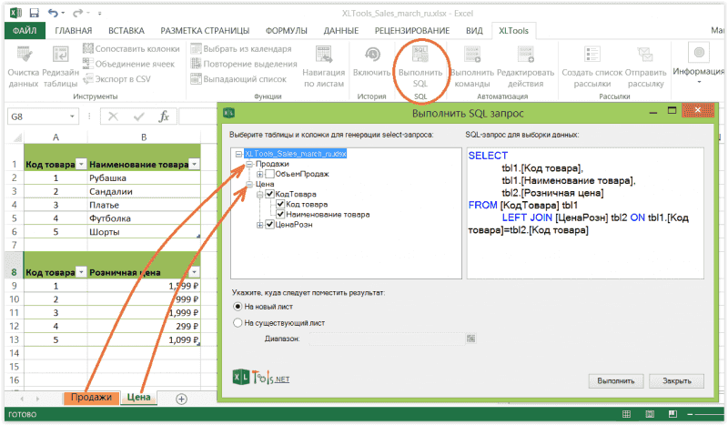
Порой таблицы Excel постепенно разрастаются настолько, что с ними становится неудобно работать. Поиск дубликатов, группировка, сложная сортировка, объединение нескольких таблиц в одну, т.д. — превращаются в действительно трудоёмкие задачи. Теоретически эти задачи можно легко решить с помощью языка запросов SQL… если бы только можно было составлять запросы напрямую к данным Excel.
Инструмент XLTools «SQL запросы» расширяет Excel возможностями языка структурированных запросов:
Перед началом работы добавьте «Всплывающие часы» в Excel
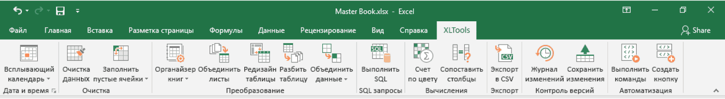
«SQL запросы» – это один из 20+ инструментов в составе надстройки XLTools для Excel. Работает в Excel 2019, 2016, 2013, 2010, десктоп Office 365.
Как превратить данные Excel в реляционную базу данных и подготовить их к работе с SQL запросами
По умолчанию Excel воспринимает данные как простые диапазоны. Но SQL применим только к реляционным базам данных. Поэтому, прежде чем создать запрос, преобразуйте диапазоны Excel в таблицу (именованный диапазон с применением стиля таблицы):
Выберите таблицу Откройте вкладку «Конструктор» Напечатайте имя таблицы.
Повторите эти шаги для каждого диапазона, который планируете использовать в запросах.
Напр., «КодТовара», «ЦенаРозн», «ОбъемПродаж», т.д.
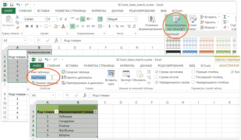
Как создать и выполнить запрос SQL SELECT к таблицам Excel
Надстройка «SQL запросы» позволяет выполнять запросы к Excel таблицам на разных листах и в разных книгах. Для этого убедитесь, что эти книги открыты, а нужные данные отформатированы как именованные таблицы.
В левой части окна находится дерево данных со всеми доступными таблицами Excel.
Нажатием на узлы открываются/сворачиваются поля таблицы (столбцы).
Выберите целые таблицы или конкретные поля.
Операторы Left Join, Order By, Group By, Distinct и другие SQLite команды в Excel
XLTools использует стандарт SQLite. Пользователи, владеющие языком SQLite, могут создавать самые разнообразные запросы:
Как объединить две и более Excel таблиц с помощью надстройки «SQL запросы»
Вы можете объединить несколько таблиц Excel в одну, если у них есть общее ключевое поле. Предположим, вам нужно объединить несколько таблиц по общему столбцу «КодТовара»:
Нажмите Выполнить SQL на вкладке XLTools Выберите поля, которые нужно включить в объединённую таблицу.
По мере выбора полей, автоматически генерируется запрос SELECT и LEFT JOIN.
Создание, загрузка и изменение запроса в Excel (Power Query)
Совет Чтобы упросить, сформированы ли данные на этом плане с помощью Power Query, выберите ячейку с данными, а если появится вкладка Лента контекстного запроса, данные загружаются из Power Query.
Знать, в какой среде вы сейчас? Power Query хорошо интегрирован с пользовательским интерфейсом Excel, особенно при импорте данных, работе с подключениями и редактировании таблиц, таблиц с Excel и именовых диапазонов. Чтобы избежать путаницы, важно в любой момент времени знать, в какой среде вы находитесь, в какой Excel или Power Query.
Знакомые Excel, лента и сетка
Лента редактора Power Query и предварительный просмотр данных
Например, работа с данными на Excel значительно отличается от Power Query. Кроме того, подключенные данные, которые вы видите на Excel, могут не работать с Power Query для их обработки. Это происходит только при загрузке данных на таблицу или в модель данных из Power Query.
Переименование я вкладок на таблицах Ямы лучше переименовывать по своему смыслу, особенно если их много. Особенно важно пояснить разницу между данными и данными, загруженными из редактора Power Query. Даже если у вас всего два листа: с таблицей Excel «Лист1»и запросом, созданным путем импорта таблицы Excel Таблица1,ее легко запутать. Всегда имеет смысл изменить названия ярлыков по умолчанию на более понятное. Например, переименуйте Лист1 в Таблицу данных и Таблицу1 в Таблицу запросов. Теперь понятно, какая вкладка с данными, а какая вкладка с запросом.
Вы можете создать запрос из импортируемых данных или пустой запрос.
Создание запроса из импортируемых данных
Это самый распространенный способ создания запроса.
Выберем ячейку в данных и выберите запрос> изменить.
Создание пустого запроса
Вы можете начать с нуля. Это можно сделать двумя способами.
Выберите Данные> Получить данные >из других источников > пустой запрос.
Выберите Данные> получить данные >запуск редактора Power Query.
На этом этапе вы можете вручную добавлять шаги и формулы, если хорошо знаете язык формул Power Query M.
Кроме того, можно выбрать команду На главная в группе Новый запрос. Выполните одно из указанных ниже действий.
Выберите Новый источник, чтобы добавить источник данных. Эта команда выглядит так же, как> «Получить данные» на Excel ленте.
Выберите Последние источники, чтобы выбрать источник данных, с помощью который вы работали. Эта команда выглядит так же, как> последние источники на Excel ленте.
Чтобы ввести данные вручную, выберите Ввести данные. Вы можете выбрать эту команду, чтобы попробовать редактор Power Query независимо от внешнего источника данных.
Предположим, что запрос действителен и не имеет ошибок, его можно загрузить обратно на таблицу или в модель данных.
Загрузка запроса из редактора Power Query
В редакторе Power Query сделайте следующее:
Чтобы загрузить на таблицу, выберите Главная> Закрыть & Загрузить > Закрыть & Загрузить.
Чтобы загрузить данные в модель данных, выберите Главная> Закрыть & Загрузить > Закрыть & Загрузка.
В диалоговом окне Импорт данных выберите добавить эти данные в модельданных.
Совет Иногда команда «Загрузить в» неатривна или отключена. Это может произойти при первом создании запроса в книге. В этом случае нажмите кнопку Закрыть & Загрузить, на новом > запросы данных & Connections > Запросы, щелкните запрос правой кнопкой мыши и выберите загрузить в . Кроме того, на ленте редактора Power Query выберите запрос> Загрузить в.
Загрузка запроса из области «Запросы и подключения»
В Excel может потребоваться загрузить запрос на другой таблицу или в модель данных.
В Excel выберите Запросы> запросы & Connections, а затем выберите вкладку Запросы.
В списке запросов найдите запрос, щелкните его правой кнопкой мыши и выберите загрузить в. Появится диалоговое окно Импорт данных.
Выберите, как вы хотите импортировать данные, а затем выберите ОК. Чтобы получить дополнительные сведения об использовании этого диалогового окна, выберите знак вопроса (?).
Существует несколько способов изменить запрос, загруженный на таблицу.
Изменение запроса на Excel данных
Чтобы изменить запрос, найдите ранее загруженную из редактора Power Query, выйдите ячейку в данных и выберите запрос > Изменить.
Изменение запроса в области «Запросы & подключения»
Возможно, вы & области Запросы и подключения удобнее использовать, если в одной книге много запросов и вы хотите быстро найти его.
В Excel выберите Запросы> запросы & Connections, а затем выберите вкладку Запросы.
В списке запросов найдите запрос, щелкните его правой кнопкой мыши и выберите изменить.
Изменение запроса в диалоговом окне «Свойства запроса»
В Excel выберите Data> Data & Connections > Запросы, щелкните запрос правой кнопкой мыши и выберите Свойства ,выберите вкладку Определение в диалоговом окне Свойства и нажмите кнопку Изменить запрос.
Совет Если вы работаете с запросом на > данных, в диалоговом окнеСвойства выберите вкладку Определение, а затем — Изменить запрос.
Модель данных обычно содержит несколько таблиц, расположенных в связи. Запрос загружается в модель данных с помощью команды Загрузить, чтобы отобразить диалоговое окно Импорт данных, а затем в поле Добавить эти данные в режим данныхl. Дополнительные сведения о моделях данных см. в дополнительных сведениях о том, какие источники данных используются в модели данных книги,Создание модели данных в Excelи Создание таблиц с помощью нескольких таблиц.
Чтобы открыть модель данных, выберите Power Pivot > Управление.
В нижней части окна Power Pivot выберите вкладку нужной таблицы.
Подтвердим, что отображается правильная таблица. Модель данных может иметь много таблиц.
Обратите внимание на имя таблицы.
Чтобы закрыть окно Power Pivot, выберите файл> Закрыть. Чтобы освободить память, может потребоваться несколько секунд.
Выберите > подключения & свойства >Запросы, щелкните запрос правой кнопкой мыши и выберите изменить.
Завершив внесение изменений в редакторе Power Query, выберите файл > Закрыть & загрузить.
Запрос на этом и в таблице в модели данных обновляются.
Если вы заметили, что загрузка запроса в модель данных занимает намного больше времени, чем загрузка на лист, проверьте действия Power Query, чтобы узнать, фильтруется ли текстовый столбец или структурированный столбец списка с помощью оператора Contains. Это действие приводит Excel повторно прогонять весь набор данных для каждой строки. Более того, Excel не могут эффективно использовать многопрочитанные выполнения. В качестве обходного решения попробуйте использовать другой оператор, например Равно или Начинает с.
Корпорация Майкрософт знает об этой проблеме и находится в стадии исследования.
Вы можете загрузить Power Query:
На один из них. В редакторе Power Query выберите Home> Close & Load > Close & Load.
В модель данных. В редакторе Power Query выберите Home> Close & Load > Close & Load To.
По умолчанию Power Query загружает запросы на новый таблицу при загрузке одного запроса и одновременно загружает несколько запросов в модель данных. Вы можете изменить поведение по умолчанию для всех книг или только для текущей книги. При настройке этих параметров Power Query не меняет результаты запроса на месте или в данных модели данных и примечаниях.
Кроме того, динамически переопределять стандартные параметры запроса можно в диалоговом окне Импорт, которое отображается после выбора параметра & Загрузитьв.
Глобальные параметры, которые применяются во всех книгах
В редакторе Power Query выберите Файл > параметры и параметры >параметры запроса.
В диалоговом окне Параметры запроса в левой части в разделе GLOBAL выберите Загрузка данных.
В разделе Загрузка Параметры запроса по умолчанию сделайте следующее:
Выберите Использовать стандартные параметры загрузки.
Выберите Указать настраиваемые параметры загрузкипо умолчанию, а затем выберите или отобирать параметр Загрузить на таблицу или Загрузить в модель данных.
Совет В нижней части диалогового окна можно выбрать восстановить параметры по умолчанию, чтобы вернуться к настройкам по умолчанию.
Параметры книги, которые применяются только к текущей книге
В диалоговом окне Параметры запроса в левой части в разделе ТЕКУЩАЯ КНИГА выберите Загрузка данных.
Выполните одно или несколько из указанных ниже действий.
В области Обнаружение типоввыберите или сберем для обнаружения типов столбцов и их заглавных колонок для неструктурированных источников.
По умолчанию они обнаруживаются. Если вы предпочитаете формировать данные самостоятельно, отоставьте этот параметр.
В области Связивыберите или отоберем создать связи между таблицами при первом добавлении в модель данных.
По умолчанию перед загрузкой в модель данных можно найти существующие связи между таблицами, например внешние ключи в реляционной базе данных, и импортировать их вместе с данными. Если вы предпочитаете делать это самостоятельно, сделайте это самостоятельно.
В области Связивыберите или отоберете update relationships when refreshing queries loaded to the Data Model (Связи) при обновлении запросов, загруженных в модель данных.
По умолчанию отношения не обновляются. При обновлении запросов, уже загруженных в модель данных, Power Query находит существующие связи между таблицами, например внешние ключи, в реляционной базе данных и обновляет их. Это может привести к удалению связей, созданных вручную после импорта данных, или к новым связям. Тем не менее, если вы хотите сделать это, выберите этот параметр.
В области Фоновыеданные выберите или отпустите разрешение предварительного просмотра данных для скачивания в фоновом режиме.
По умолчанию предварительный просмотр данных загружается в фоновом режиме. Если вы хотите сразу же видеть все данные, отобираем этот параметр.
Запрос на выборку данных (формулы) в EXCEL
Суть запроса на выборку – выбрать из исходной таблицы строки, удовлетворяющие определенным критериям (подобно применению стандартного Фильтра ). Произведем отбор значений из исходной таблицы с помощью формул массива . В отличие от применения Фильтра ( CTRL+SHIFT+L или Данные/ Сортировка и фильтр/ Фильтр ) отобранные строки будут помещены в отдельную таблицу.
В этой статье рассмотрим наиболее часто встречающиеся запросы, например: отбор строк таблицы, у которых значение из числового столбца попадает в заданный диапазон (интервал); отбор строк, у которых дата принаждежит определенному периоду; задачи с 2-мя текстовыми критериями и другие. Начнем с простых запросов.
1. Один числовой критерий (Выбрать те Товары, у которых цена выше минимальной)
Пусть имеется Исходная таблица с перечнем Товаров и Ценами (см. файл примера, лист Один критерий — число ).
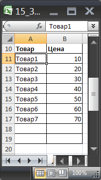
Необходимо отобразить в отдельной таблице только те записи (строки) из Исходной таблицы, у которых цена выше 25.
Решить эту и последующие задачи можно легко с помощью стандартного фильтра . Для этого выделите заголовки Исходной таблицы и нажмите CTRL+SHIFT+L . Через выпадающий список у заголовка Цены выберите Числовые фильтры. , затем задайте необходимые условия фильтрации и нажмите ОК.
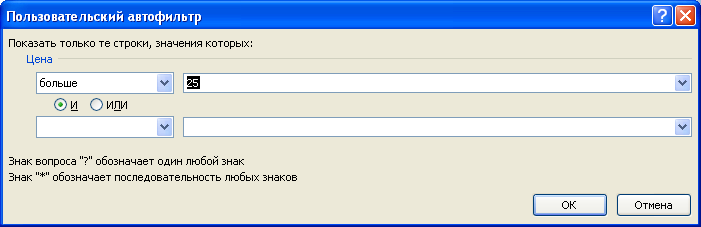
Будут отображены записи удовлетворяющие условиям отбора.
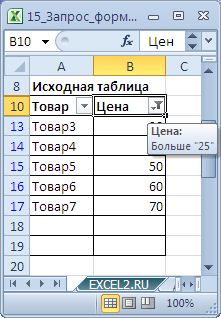
Другим подходом является использование формул массива . В отличие от фильтра отобранные строки будут помещены в отдельную таблицу — своеобразный Отчет , который, например, можно отформатировать в стиль отличный от Исходной таблицы или производить другие ее модификации.
Критерий (минимальную цену) разместим в ячейке Е6 , таблицу для отфильтрованных данных — в диапазоне D10:E19 .
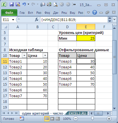
Теперь выделим диапазон D11:D19 (столбец Товар) и в Строке формул введем формулу массива :
Вместо ENTER нажмите сочетание клавиш CTRL+SHIFT+ENTER .
Те же манипуляции произведем с диапазоном E11:E19 куда и введем аналогичную формулу массива :
В результате получим новую таблицу, которая будет содержать только товары, у которых цены попадают в интервал, указанный в ячейках Е5 и Е6 .
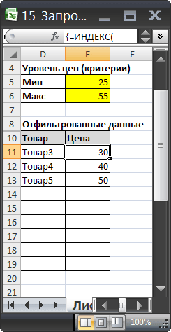
Чтобы показать динамизм полученного Отчета (Запроса на выборку) введем в Е6 значение 65. В новую таблицу будет добавлена еще одна запись из Исходной таблицы, удовлетворяющая новому критерию.
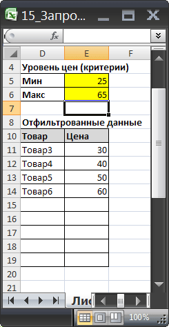
Если в Исходную таблицу добавить новый товар с Ценой в диапазоне от 25 до 65, то в новую таблицу будет добавлена новая запись.
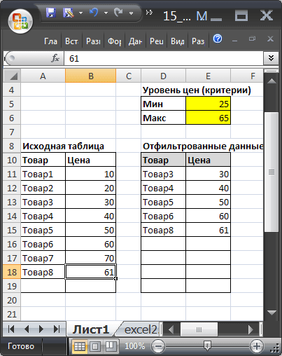
В файле примера также содержатся формулы массива с обработкой ошибок, когда в столбце Цена содержится значение ошибки, например #ДЕЛ/0! (см. лист Обработка ошибок ).
Следующие задачи решаются аналогичным образом, поэтому не будем их рассматривать так детально.
3. Один критерий Дата (Выбрать те Товары, у которых Дата поставки совпадает заданной)
Пусть имеется Исходная таблица с перечнем Товаров и Датами поставки (см. файл примера, лист Один критерий — Дата ).
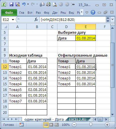
Для отбора строк используются формулы массива, аналогичные Задаче1 (вместо критерия =$B$12:$B$20)*(СТРОКА($B$12:$B$20)-СТРОКА($B$11));$J$12-СТРОКА(A12)+СТРОКА($B$11)+1))
Примечание : После ввода формулы вместо клавиши ENTER (ВВОД) нужно нажать сочетание клавиш CTRL+SHIFT+ENTER. Это сочетание клавиш используется для ввода формул массива.
Скопируйте формулу массива вниз на нужное количество ячеек. Формула вернет только те значения Товаров, которые были поставлены в диапазоне указанных дат. В остальных ячейках будут содержаться ошибки #ЧИСЛО! Ошибки в файле примера (Лист 4.Диапазон Дат) скрыты с помощью Условного форматирования .
Аналогичную формулу нужно ввести и для дат в столбец E.
В ячейке J12 вычислено количество строк исходной таблицы, удовлетворяющих критериям:
Решение2 : Для отбора строк можно использовать формулы массива, аналогичные Задаче2 (т.е. формулы массива, возвращающие несколько значений ):
Для ввода первой формулы выделите диапазон ячеек G12:G20 . После ввода формулы вместо клавиши ENTER (ВВОД) нужно нажать сочетание клавиш CTRL+SHIFT+ENTER.
Решение3 : Если столбец Дат СОРТИРОВАН, то можно не использовать формулы массива.
Сначала необходимо вычислить первую и последнюю позиции строк, которые удовлетворяют критериям. Затем вывести строки с помощью функции СМЕЩ() .
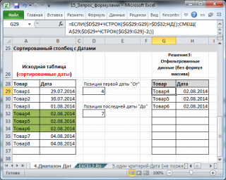
Этот пример еще раз наглядно демонстрирует насколько предварительная сортировка данных облегчает написание формул.
5. Один критерий Дата (Выбрать те Товары, у которых Дата поставки не раньше/ не позже заданной)
Пусть имеется Исходная таблица с перечнем Товаров и Датами поставки (см. файл примера, лист Один критерий — Дата (не позже) ).
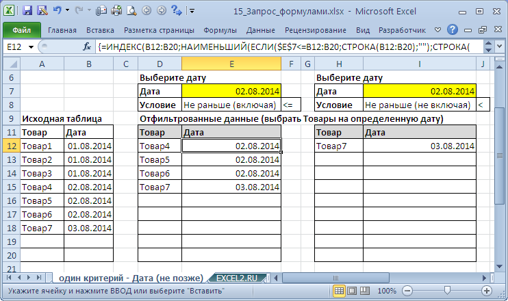
Для отбора строк, дата которых не раньше (включая саму дату), используется формула массива:
= ИНДЕКС(A12:A20;НАИМЕНЬШИЙ(ЕСЛИ($E$7 C15;И($B$7>=B15;$B$7 =$B$13:$B$21)*($B$13:$B$21>0);СТРОКА($B$13:$B$21);»»);СТРОКА($B$13:$B$21)-СТРОКА($B$12)) -СТРОКА($B$12))
Условие $E$7=$A$13:$A$21 гарантирует, что будут отобраны товары только определенного типа. Условие $E$8>=$B$13:$B$21 гарантирует, что будут отобраны даты не позже заданной (включая). Условие $B$13:$B$21>0 необходимо, если в диапазоне дат имеются пустые ячейки. Знак * (умножение) используется для задания Условия И (все 3 критерия должны выполняться для строки одновременно).
Примечание . Случай, когда список несортирован, рассмотрен в статье Поиск ДАТЫ (ЧИСЛА) ближайшей к заданной, с условием в MS EXCEL. Несортированный список .
7. Один Текстовый критерий (Выбрать Товары определенного вида)
Пусть имеется Исходная таблица с перечнем Товаров и Ценами (см. файл примера, лист Один критерий — Текст ).
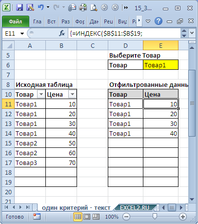
Задача решается аналогично Задачам 1 и 3. Более подробное решение см. в статье Поиск ТЕКСТовых значений в MS EXCEL с выводом их в отдельный список. Часть1. Обычный поиск .
8. Два Текстовых критерия (Выбрать Товары определенного вида, поставленные в заданный месяц)
Пусть имеется Исходная таблица с перечнем Товаров и Ценами (см. файл примера, лист 2 критерия — текст (И) ).
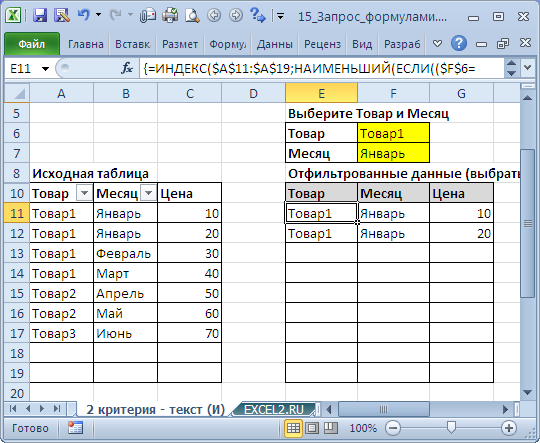
Для отбора строк используется формула массива:
Выражение ($F$6=$A$11:$A$19)*($F$7=$B$11:$B$19) задает оба условия (Товар и Месяц).
Выражение СТРОКА(ДВССЫЛ(«A1:A»&ЧСТРОК($A$11:$A$19))) формирует массив последовательных чисел , т.е. номера строк в таблице.
9. Два Текстовых критерия (Выбрать Товары определенных видов)
Пусть имеется Исходная таблица с перечнем Товаров и Ценами (см. файл примера, лист 2 критерия — текст (ИЛИ) ).
В отличие от Задачи 7 отберем строки с товарами 2-х видов ( Условие ИЛИ ).
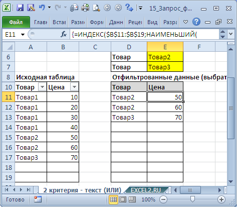
Для отбора строк используется формула массива:
= ИНДЕКС(A$11:A$19; НАИБОЛЬШИЙ((($E$6=$A$11:$A$19)+($E$7=$A$11:$A$19))*(СТРОКА($A$11:$A$19)-СТРОКА($A$10)); СЧЁТЕСЛИ($A$11:$A$19;$E$6)+СЧЁТЕСЛИ($A$11:$A$19;$E$7)-ЧСТРОК($A$11:A11)+1))
Условие ($E$6=$A$11:$A$19)+($E$7=$A$11:$A$19) гарантирует, что будут отобраны товары только заданных видов из желтых ячеек (Товар2 и Товар3). Знак + (сложение) используется для задания Условие ИЛИ (должен быть выполнен хотя бы 1 критерий).
Вышеуказанное выражение вернет массив . Умножив его на выражение СТРОКА($A$11:$A$19)-СТРОКА($A$10) , т.е. на массив последовательных чисел , получим массив позиций (номеров строк таблицы), удовлетворяющих критериям. В нашем случае это будет массив .
С помощью функции НАИБОЛЬШИЙ() выведем 3 значения из позиции 5 (строка 15 листа), 6 (16) и 7 (17), т.е. значения Товар2, Товар2 и Товар3. Для этого используем выражение СЧЁТЕСЛИ($A$11:$A$19;$E$6)+СЧЁТЕСЛИ($A$11:$A$19;$E$7)-ЧСТРОК($A$11:A11)+1 , которое последовательно (начиная со строки 11) будет возвращать числа 3; 2; 1; 0; -1; -2; . Формула НАИБОЛЬШИЙ(. ;3) вернет число 5, НАИБОЛЬШИЙ(. ;2) вернет число 6, НАИБОЛЬШИЙ(. ;1) вернет число 7, а НАИБОЛЬШИЙ(. ;0) и далее вернет ошибку, которую мы скроем условным форматированием .
И наконец, с помощью функции ИНДЕКС() последовательно выведем наши значения из соответствующих позиций: = ИНДЕКС(A$11:A$19;5) вернет Товар2, = ИНДЕКС(A$11:A$19;6) вернет Товар2, = ИНДЕКС(A$11:A$19;7) вернет Товар3.
10. Отбор значений с учетом повторов
В разделе Отбор на основании повторяемости собраны статьи о запросах с группировкой данных. Из повторяющихся данных сначала отбираются уникальные значения, а соответствующие им значения в других столбцах — группируются (складываются, усредняются и пр.).
Наиболее популярные статьи из этого раздела:
В качестве примера приведем решения следующей задачи: Выбрать Товары, цена которых лежит в определенном диапазоне и повторяется заданное количество раз или более.
В качестве исходной возьмем таблицу партий товаров.
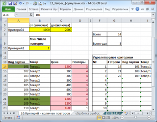
Предположим, что нас интересует сколько и каких партий товаров поставлялось по цене от 1000р. до 2000р. (критерий 1). Причем, партий с одинаковой ценой должно быть минимум 3 (критерий 2).
Решением является формула массива:
Эта формула возвращает номера строк, которые удовлетворяют обоим критериям.
Формула =СУММПРОИЗВ(($C$14:$C$27>=$B$7)*($C$14:$C$27 =$B$10)) подсчитывает количество строк, которые удовлетворяют критериям.
В файле примера на листе «10.Критерий — колич-во повторов» настроено Условное форматирование , которое позволяет визуально определить строки удовлетворяющие критериям, а также скрыть ячейки, в которых формула массива возвращает ошибку #ЧИСЛО!
11. Используем значение критерия (Любой) или (Все)
В фильтре Сводных таблиц MS EXCEL используется значение (Все), чтобы вывести все значения столбца. Другими словами, в выпадающем списке значений критерия содержится особое значение, которое отменяет сам критерий (см. статью Отчеты в MS EXCEL , Отчет №3).
В файле примера на листе «11. Критерий Любой или (Все)» реализован данный вариант критерия.
Формула в этом случае должна содержать функцию ЕСЛИ() . Если выбрано значение (Все), то используется формула для вывода значений без учета данного критерия. Если выбрано любое другое значение, то критерий работает обычным образом.
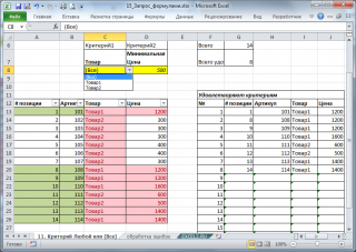
Остальная часть формулы аналогична рассмотренным выше.
12. Актуальная цена
Пусть для товара ежедневно заполняется таблица цен (цена может меняться, но не каждый день). Нужно найти актуальнуй цену, т.е. цену на последнюю дату. Если товар всего один, то можно отсортировать по дате и в последней строке будет нужная актуальная цена. Если товаров много, то нужно сначала выбрать Автофильтром нужный товар, затем опять отсортировать по цене.
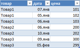
Чтобы иметь перечень товаров с актуальными ценами придется использовать формулы:
2) определяем последнюю (максимальную) дату для каждого товара с помощью формулы массива =МАКС((Таблица1[товар]=E8)*Таблица1[дата])
3) наконец, выводим актуальную цену =СУММЕСЛИМН(Таблица1[цена];Таблица1[товар];E8;Таблица1[дата];F8)
Для товара не должно быть повторов дат, иначе цены будут суммироваться (если повторяется последняя дата).
This post looks at how to use the Power Query editor to edit existing queries in Excel. We’ve seen some of this in a previous post of this Power Query series, but now we’ll go a lot deeper.
Download the example file
I recommend you download the example file for this post. Then you’ll be able to work along with examples and see the solution in action, plus the file will be useful for future reference.
![]()
Download the file: 0091 Example 7 – Edit Queries.xlsx
All the examples in this post use 0091 Example 7 – Edit Queries.xlsx. So, open up the file, and let’s get going.
As with many features of Power Query, there are multiple ways to access the same action. Opening the Power Query editor to edit an existing query is no different; there are loads of ways to do it. I will briefly cover the most common below, though we only need to know one or two.
Queries & Connections
In my opinion, the easiest place to open the Power Query editor is from the Queries and Connections pane. Click Data > Queries & Connections from the ribbon.
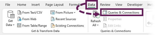
The Queries & Connections pane opens. Even within here are three ways to open the Power Query editor:
- Double-click on the name of a query.
- Right-click on the query and select edit.
- Hover over a query name (don’t click, just hover), Excel displays the query summary. Click the Edit option at the bottom.
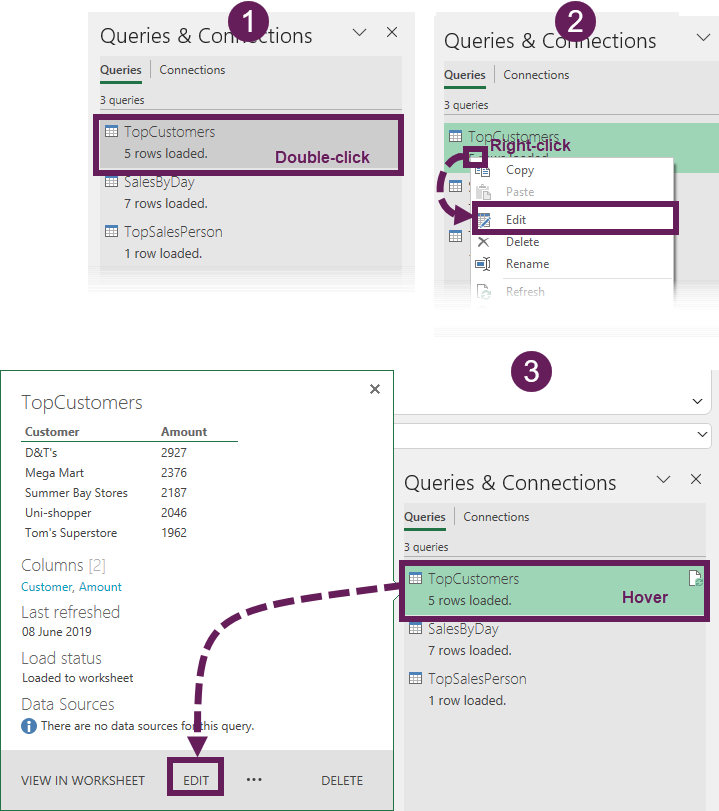
All 3 of these options will get you into the Power Query editor.
Launch Power Query editor
We can get directly into the Power Query editor from the ribbon; we don’t need to select any specific query. Click Data > Get Data > Launch Power Query Editor….
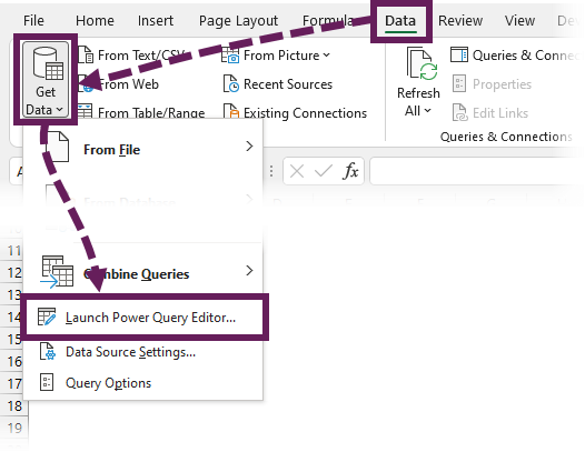
Query ribbon
Clicking on a Table containing a query (green striped format by default) will reveal the Query ribbon. Then, Click Query > Edit.
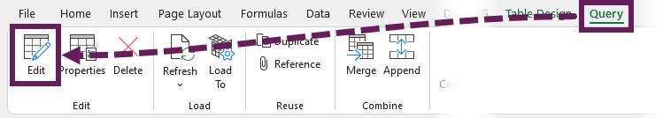
Also, right-clicking on a Table and selecting Table > Edit Query can get to the query editor.
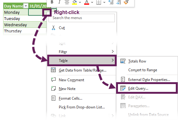
Inside the Power Query editor
Once the Power Query editor opens, we can edit any query in the workbook. If the queries pane on the left is closed, click on the > arrow to expand the list. Once the queries pane is open, click on any individual query to activate it for viewing or editing.
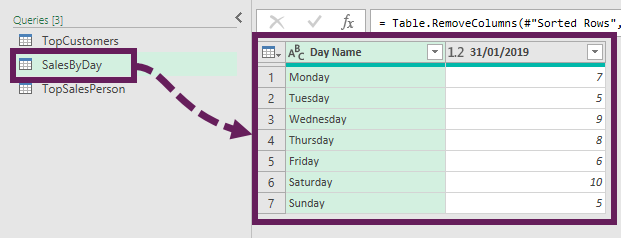
Edit transformations
Now that we’ve selected a query, we are ready to start editing. For the remainder of this post, we are working with the example file. We will to modify the existing from that file transformations.
Use one of the methods above for opening Power Query, then we can get started editing transformations.
Basic settings
The gear icon exists next to many of the steps within the applied steps list. Clicking the icon reveals the options window for that specific step.
Using the Example file, select the Top Customers query, then click on the gear icon next to the Keep First Rows step. The Keep Top Rows window opens. The query is currently set to show 5 customers, change this to 3, and click OK.
![]()
Woop, Woop! We have just edited the query.
Adding steps
The applied steps box is also used to insert, move and delete steps. Let’s take a look at that in this section.
Select the TopCustomers query and click on the step called Calculated End of Month. The data preview shows all the transformation steps up to the end of the current selection.
Now let’s insert a new step. Click on the filter drop-down of the Date column and select only 31 January 2019 (depending on your local date format it may appear slightly different for you). Then, click OK.
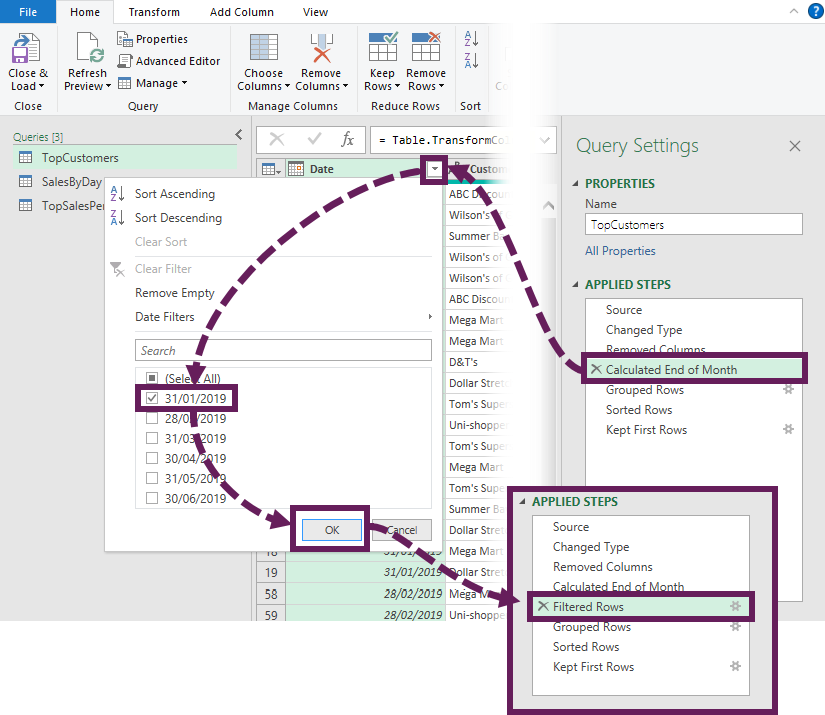
A new step appears below the previously selected step.
Clicking through the remaining steps to view the transformations, there should be no issues with this specific example. However, this will not always be the case. When changing steps in the middle of a query, it can cause errors later on, as the changes we make may not flow through into the subsequent steps.
Click on the Removed Columns step. Change the header of the Date column to Month End.
A warning message is displayed. Not all warning messages are bad; you get to choose if it is relevant to your scenario or not. We are trying to force an error in this example, so please click Insert.
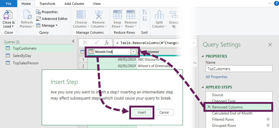
The new step is added.
Next, click on the Calculated End of Month step. Oh dear… there is an error. This is because the Calculated End of Month step is trying to find a column called Date, which is no longer exists (we renamed it to Month End Date). If you still have the Formula Bar open, you can see the reference to the Date column, which is no longer available (see the screenshot below).
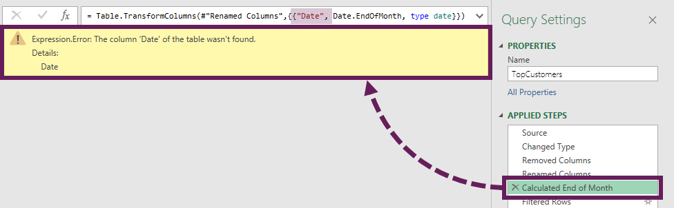
Now we have some choices. Do we need to insert that step at this point? Should we delete and re-perform the affected steps? Should we edit the M code of the remaining steps to replicate the change? Only you can make this decision.
Once you’ve been in this situation a few times, you’ll soon work out the best options. I recommend only deleting the remaining steps and re-performing the transformations as a last resort. With some practice and perseverance, you’ll learn how to fix the most common errors by using the formula bar or inserting additional steps.
Deleting steps
The example above illustrates the potential issues from editing existing steps; let’s delete the Renamed Columns step that we added. Click on the X next to the step to remove it.
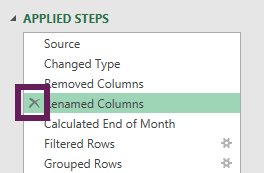
Deleting is easy, but be aware that this can cause errors too.
Moving steps
To move a step up or down, there are again more user-interface options:
- Right-click on the step and click Move Up or Move Down from the menu (see screenshot below)
- Click on a single step, hold the mouse button down and drag the step to a new location. This is my preferred option.
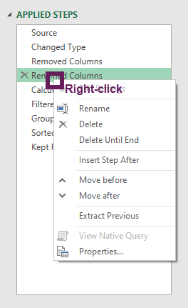
As you can imagine, moving steps has the same issues as inserting steps; it can result in errors.
Where did my step go?
Power Query is smart; it groups similar actions together where it can.
Select the SalesByDay query and ensure you have selected the last step, which is Removed Columns1. Now, let us change the headers of each column:
- Change Day Name to Day – a new step is added.
- Change 31/01/2019 (or your local date equivalent) to Number of Sales – a new step is not added.
Look at the applied steps again… there is only one step added. Where did the second step go?
Take a closer look at the Formula Bar; you will see that both the steps have been combined into one.
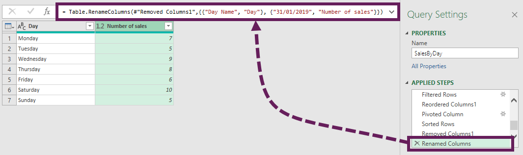
This occurs when like-for-like steps are performed one after another. It certainly helps to keep the applied steps significantly smaller than they might be otherwise.
M code: Formula bar & Advanced Editor
OK, things are about to get serious – we are going to edit the M code! We can edit the code directly in two ways:
- Formula Bar
- Advanced Editor.
I prefer the Formula Bar method. So, let’s start there.
Formula bar
If the formula bar is not visible, we can turn it on by clicking View > Formula Bar from the ribbon.
Select the SalesByDay query and click on the Sorted Rows step.
The formula bar will show the following:
![]()
Even though might not be able to write M code from scratch, but that doesn’t mean we can’t edit the code with a bit of common sense. In the formula bar, change the text “Day of Week” to “Day Name”. If you look at the data preview window, the Day Name column is now sorted in ascending order.
Next, change the text which says Order.Ascending to Order.Descending. Check the preview window again, and notice the order has changed.
The final formula should look like this:
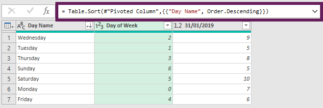
See, it’s not so difficult to edit the M code after all 😀
Advanced Editor
The changes we saw above can also be applied in the Advanced Editor. Click on Home > Advanced Editor.
The Advanced Editor shows every step in the query. First, we need to identify the relevant code. To do this look down the left side of the code. In the applied steps the step was called Sort Rows in the Power Query editor it is the #”Sort Rows” steps we require.
We can then make the same changes as noted in the formula bar section above (see the highlighted section below).
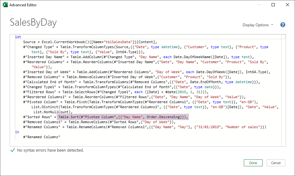
Close and Load into Excel
Finally, let’s close this out by clicking Close and Load. The changes we’ve made are refreshed into the Tables on the worksheet.
An important point to note is that Close & Load does not just apply to the active query, but to all queries in the workbook. So, if we’ve edited multiple queries due the session, they will all be updated simultaneously.
Close without saving changes
After editing a query, we may decide we don’t want to load the changes into Excel. To discard the changes, click File > Discard and Close.
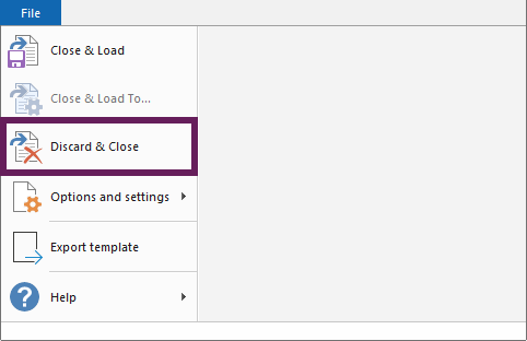
Alternatively, we can click the [X] close button (top right of the window). A confirmation box ensures we don’t lose our changes by mistake. Clicking Discard returns us back to Excel without making any changes.
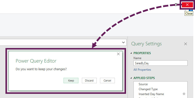
Wrap-up
This post shows us how to open and edit within the Power Query editor. While we have only made basic transformations, the methods shown apply to more advanced transformations too.
Read more posts in this series
- Introduction to Power Query
- Get data into Power Query – 5 common data sources
- DataRefresh Power Query in Excel: 4 ways & advanced options
- Use the Power Query editor to update queries
- Get to know Power Query Close & Load options
- Power Query Parameters: 3 methods
- Common Power Query transformations (50+ powerful transformations explained)
- Power Query Append: Quickly combine many queries into 1
- Get data from folder in Power Query: combine files quickly
- List files in a folder & subfolders with Power Query
- How to get data from the Current Workbook with Power Query
- How to unpivot in Excel using Power Query (3 ways)
- Power Query: Lookup value in another table with merge
- How to change source data location in Power Query (7 ways)
- Power Query formulas (how to use them and pitfalls to avoid)
- Power Query If statement: nested ifs & multiple conditions
- How to use Power Query Group By to summarize data
- How to use Power Query Custom Functions
- Power Query – Common Errors & How to Fix Them
- Power Query – Tips and Tricks

About the author
Hey, I’m Mark, and I run Excel Off The Grid.
My parents tell me that at the age of 7 I declared I was going to become a qualified accountant. I was either psychic or had no imagination, as that is exactly what happened. However, it wasn’t until I was 35 that my journey really began.
In 2015, I started a new job, for which I was regularly working after 10pm. As a result, I rarely saw my children during the week. So, I started searching for the secrets to automating Excel. I discovered that by building a small number of simple tools, I could combine them together in different ways to automate nearly all my regular tasks. This meant I could work less hours (and I got pay raises!). Today, I teach these techniques to other professionals in our training program so they too can spend less time at work (and more time with their children and doing the things they love).
Do you need help adapting this post to your needs?
I’m guessing the examples in this post don’t exactly match your situation. We all use Excel differently, so it’s impossible to write a post that will meet everybody’s needs. By taking the time to understand the techniques and principles in this post (and elsewhere on this site), you should be able to adapt it to your needs.
But, if you’re still struggling you should:
- Read other blogs, or watch YouTube videos on the same topic. You will benefit much more by discovering your own solutions.
- Ask the ‘Excel Ninja’ in your office. It’s amazing what things other people know.
- Ask a question in a forum like Mr Excel, or the Microsoft Answers Community. Remember, the people on these forums are generally giving their time for free. So take care to craft your question, make sure it’s clear and concise. List all the things you’ve tried, and provide screenshots, code segments and example workbooks.
- Use Excel Rescue, who are my consultancy partner. They help by providing solutions to smaller Excel problems.
What next?
Don’t go yet, there is plenty more to learn on Excel Off The Grid. Check out the latest posts: