Python pandas read from excel - Word и Excel - помощь в работе с программами

Excel sheets are very instinctive and user-friendly, which makes them ideal for manipulating large datasets even for less technical folks. If you are looking for places to learn to manipulate and automate stuff in excel files using Python, look no more. You are at the right place.

Python Pandas With Excel Sheet

In this article, you will learn how to use Pandas to work with Excel spreadsheets. At the end of the article, you will have the knowledge of:

Necessary modules are needed for this and how to set them up in your system.
Reading data from excel files into pandas using Python.
Exploring the data from excel files in Pandas.
Using functions to manipulate and reshape the data in Pandas.

Installation

To install Pandas in Anaconda, we can use the following command in Anaconda Terminal:

conda install pandas

To install Pandas in regular Python (Non-Anaconda), we can use the following command in the command prompt:

pip install pandas

Getting Started

First of all, we need to import the Pandas module which can be done by running the command: Pandas

Python3

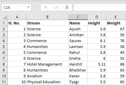
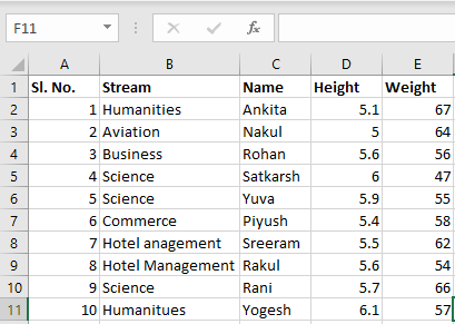
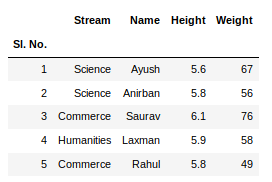
Input File: Let’s suppose the excel file looks like this

Sheet 1:

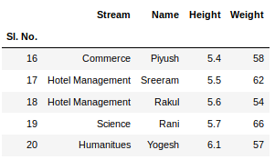
Sheet 2:

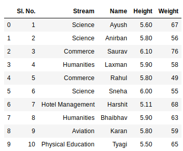
Now we can import the excel file using the read_excel function in Pandas. The second statement reads the data from excel and stores it into a pandas Data Frame which is represented by the variable newData. If there are multiple sheets in the excel workbook, the command will import data of the first sheet. To make a data frame with all the sheets in the workbook, the easiest method is to create different data frames separately and then concatenate them. The read_excel method takes argument sheet_name and index_col where we can specify the sheet of which the data frame should be made of and index_col specifies the title column, as is shown below:

Python3

file =('path_of_excel_file')

newData = pds.read_excel(file)

newData

Output:

Example:

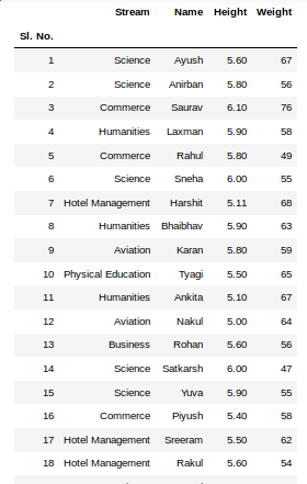
The third statement concatenates both sheets. Now to check the whole data frame, we can simply run the following command:

Python3

sheet1 = pds.read_excel(file,

sheet_name = 0,

index_col = 0)

sheet2 = pds.read_excel(file,

sheet_name = 1,

index_col = 0)

newData = pds.concat([sheet1, sheet2])

newData

Output:

To view 5 columns from the top and from the bottom of the data frame, we can run the command. This head() and tail() method also take arguments as numbers for the number of columns to show.

Python3

newData.head()

newData.tail()

Output:

The shape() method can be used to view the number of rows and columns in the data frame as follows:

Python3

Output:

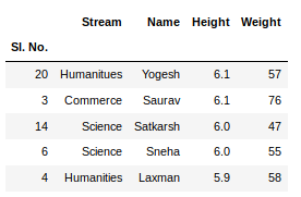
If any column contains numerical data, we can sort that column using the sort_values() method in pandas as follows:

Python3

sorted_column = newData.sort_values(['Height'], ascending = False)

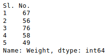
Now, let’s suppose we want the top 5 values of the sorted column, we can use the head() method here:

Python3

sorted_column['Height'].head(5)

Output:

We can do that with any numerical column of the data frame as shown below:

Python3

Output:

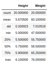
Now, suppose our data is mostly numerical. We can get the statistical information like mean, max, min, etc. about the data frame using the describe() method as shown below:

Python3

Output:

This can also be done separately for all the numerical columns using the following command:

Python3

Output:

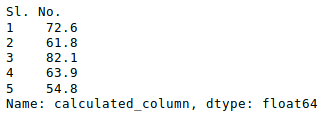
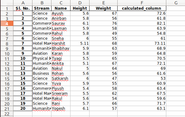
Other statistical information can also be calculated using the respective methods. Like in excel, formulas can also be applied and calculated columns can be created as follows:

Python3

newData['calculated_column'] =

newData[“Height”] + newData[“Weight”]

newData['calculated_column'].head()

Output:

After operating on the data in the data frame, we can export the data back to an excel file using the method to_excel. For this we need to specify an output excel file where the transformed data is to be written, as shown below:

Python3

newData.to_excel('Output File.xlsx')

Output:

Источник

Why learn to work with Excel with Python? Excel is one of the most popular and widely-used data tools; it’s hard to find an organization that doesn’t work with it in some way. From analysts, to sales VPs, to CEOs, various professionals use Excel for both quick stats and serious data crunching.

With Excel being so pervasive, data professionals must be familiar with it. Working with data in Python or R offers serious advantages over Excel’s UI, so finding a way to work with Excel using code is critical. Thankfully, there’s a great tool already out there for using Excel with Python called pandas.

Pandas has excellent methods for reading all kinds of data from Excel files. You can also export your results from pandas back to Excel, if that’s preferred by your intended audience. Pandas is great for other routine data analysis tasks, such as:

quick Exploratory Data Analysis (EDA)
drawing attractive plots
feeding data into machine learning tools like scikit-learn
building machine learning models on your data
taking cleaned and processed data to any number of data tools

Pandas is better at automating data processing tasks than Excel, including processing Excel files.

In this tutorial, we are going to show you how to work with Excel files in pandas. We will cover the following concepts.

setting up your computer with the necessary software
reading in data from Excel files into pandas
data exploration in pandas
visualizing data in pandas using the matplotlib visualization library
manipulating and reshaping data in pandas
moving data from pandas into Excel

Note that this tutorial does not provide a deep dive into pandas. To explore pandas more, check out our course.

System Prerequisites

We will use Python 3 and Jupyter Notebook to demonstrate the code in this tutorial.In addition to Python and Jupyter Notebook, you will need the following Python modules:

matplotlib — data visualization
NumPy — numerical data functionality
OpenPyXL — read/write Excel 2010 xlsx/xlsm files
pandas — data import, clean-up, exploration, and analysis
xlrd — read Excel data
xlwt — write to Excel
XlsxWriter — write to Excel (xlsx) files

There are multiple ways to get set up with all the modules. We cover three of the most common scenarios below.

If you have Python installed via Anaconda package manager, you can install the required modules using the command conda install. For example, to install pandas, you would execute the command — conda install pandas.
If you already have a regular, non-Anaconda Python installed on the computer, you can install the required modules using pip. Open your command line program and execute command pip install <module name> to install a module. You should replace <module name> with the actual name of the module you are trying to install. For example, to install pandas, you would execute command — pip install pandas.
If you don’t have Python already installed, you should get it through the Anaconda package manager. Anaconda provides installers for Windows, Mac, and Linux Computers. If you choose the full installer, you will get all the modules you need, along with Python and pandas within a single package. This is the easiest and fastest way to get started.

The Data Set

In this tutorial, we will use a multi-sheet Excel file we created from Kaggle’s IMDB Scores data. You can download the file here.

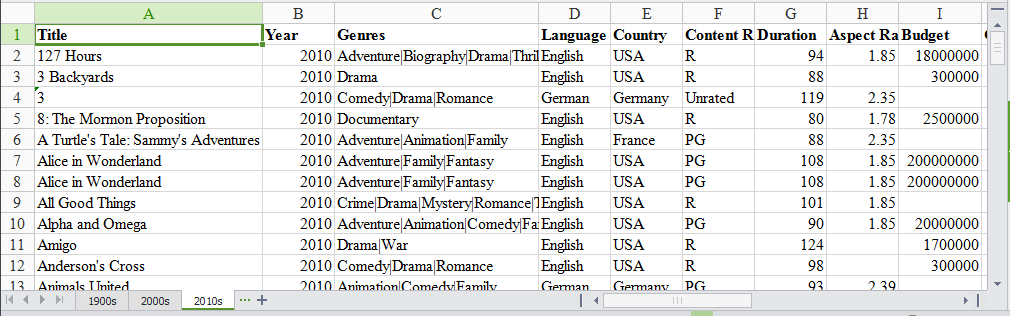
Our Excel file has three sheets: ‘1900s,’ ‘2000s,’ and ‘2010s.’ Each sheet has data for movies from those years.

We will use this data set to find the ratings distribution for the movies, visualize movies with highest ratings and net earnings and calculate statistical information about the movies. We will be analyzing and exploring this data using Python and pandas, thus demonstrating pandas capabilities for working with Excel data in Python.

Read data from the Excel file

We need to first import the data from the Excel file into pandas. To do that, we start by importing the pandas module.

import pandas as pd

We then use the pandas’ read_excel method to read in data from the Excel file. The easiest way to call this method is to pass the file name. If no sheet name is specified then it will read the first sheet in the index (as shown below).

excel_file = 'movies.xls'
movies = pd.read_excel(excel_file)

Here, the read_excel method read the data from the Excel file into a pandas DataFrame object. Pandas defaults to storing data in DataFrames. We then stored this DataFrame into a variable called movies.

Pandas has a built-in DataFrame.head() method that we can use to easily display the first few rows of our DataFrame. If no argument is passed, it will display first five rows. If a number is passed, it will display the equal number of rows from the top.

movies.head()

	Title	Year	Genres	Language	Country	Content Rating	Duration	Aspect Ratio	Budget	Gross Earnings	…	Facebook Likes — Actor 1	Facebook Likes — Actor 2	Facebook Likes — Actor 3	Facebook Likes — cast Total	Facebook likes — Movie	Facenumber in posters	User Votes	Reviews by Users	Reviews by Crtiics	IMDB Score
0	Intolerance: Love’s Struggle Throughout the Ages	1916	Drama\|History\|War	NaN	USA	Not Rated	123	1.33	385907.0	NaN	…	436	22	9.0	481	691	1	10718	88	69.0	8.0
1	Over the Hill to the Poorhouse	1920	Crime\|Drama	NaN	USA	NaN	110	1.33	100000.0	3000000.0	…	2	2	0.0	4	0	1	5	1	1.0	4.8
2	The Big Parade	1925	Drama\|Romance\|War	NaN	USA	Not Rated	151	1.33	245000.0	NaN	…	81	12	6.0	108	226	0	4849	45	48.0	8.3
3	Metropolis	1927	Drama\|Sci-Fi	German	Germany	Not Rated	145	1.33	6000000.0	26435.0	…	136	23	18.0	203	12000	1	111841	413	260.0	8.3
4	Pandora’s Box	1929	Crime\|Drama\|Romance	German	Germany	Not Rated	110	1.33	NaN	9950.0	…	426	20	3.0	455	926	1	7431	84	71.0	8.0

5 rows × 25 columns

Excel files quite often have multiple sheets and the ability to read a specific sheet or all of them is very important. To make this easy, the pandas read_excel method takes an argument called sheetname that tells pandas which sheet to read in the data from. For this, you can either use the sheet name or the sheet number. Sheet numbers start with zero. If the sheetname argument is not given, it defaults to zero and pandas will import the first sheet.

By default, pandas will automatically assign a numeric index or row label starting with zero. You may want to leave the default index as such if your data doesn’t have a column with unique values that can serve as a better index. In case there is a column that you feel would serve as a better index, you can override the default behavior by setting index_col property to a column. It takes a numeric value for setting a single column as index or a list of numeric values for creating a multi-index.

In the below code, we are choosing the first column, ‘Title’, as index (index=0) by passing zero to the index_col argument.

movies_sheet1 = pd.read_excel(excel_file, sheetname=0, index_col=0)
movies_sheet1.head()

	Year	Genres	Language	Country	Content Rating	Duration	Aspect Ratio	Budget	Gross Earnings	Director	…	Facebook Likes — Actor 1	Facebook Likes — Actor 2	Facebook Likes — Actor 3	Facebook Likes — cast Total	Facebook likes — Movie	Facenumber in posters	User Votes	Reviews by Users	Reviews by Crtiics	IMDB Score
Title
Intolerance: Love’s Struggle Throughout the Ages	1916	Drama\|History\|War	NaN	USA	Not Rated	123	1.33	385907.0	NaN	D.W. Griffith	…	436	22	9.0	481	691	1	10718	88	69.0	8.0
Over the Hill to the Poorhouse	1920	Crime\|Drama	NaN	USA	NaN	110	1.33	100000.0	3000000.0	Harry F. Millarde	…	2	2	0.0	4	0	1	5	1	1.0	4.8
The Big Parade	1925	Drama\|Romance\|War	NaN	USA	Not Rated	151	1.33	245000.0	NaN	King Vidor	…	81	12	6.0	108	226	0	4849	45	48.0	8.3
Metropolis	1927	Drama\|Sci-Fi	German	Germany	Not Rated	145	1.33	6000000.0	26435.0	Fritz Lang	…	136	23	18.0	203	12000	1	111841	413	260.0	8.3
Pandora’s Box	1929	Crime\|Drama\|Romance	German	Germany	Not Rated	110	1.33	NaN	9950.0	Georg Wilhelm Pabst	…	426	20	3.0	455	926	1	7431	84	71.0	8.0

5 rows × 24 columns

As you noticed above, our Excel data file has three sheets. We already read the first sheet in a DataFrame above. Now, using the same syntax, we will read in rest of the two sheets too.

movies_sheet2 = pd.read_excel(excel_file, sheetname=1, index_col=0)
movies_sheet2.head()

	Year	Genres	Language	Country	Content Rating	Duration	Aspect Ratio	Budget	Gross Earnings	Director	…	Facebook Likes — Actor 1	Facebook Likes — Actor 2	Facebook Likes — Actor 3	Facebook Likes — cast Total	Facebook likes — Movie	Facenumber in posters	User Votes	Reviews by Users	Reviews by Crtiics	IMDB Score
Title
102 Dalmatians	2000	Adventure\|Comedy\|Family	English	USA	G	100.0	1.85	85000000.0	66941559.0	Kevin Lima	…	2000.0	795.0	439.0	4182	372	1	26413	77.0	84.0	4.8
28 Days	2000	Comedy\|Drama	English	USA	PG-13	103.0	1.37	43000000.0	37035515.0	Betty Thomas	…	12000.0	10000.0	664.0	23864	0	1	34597	194.0	116.0	6.0
3 Strikes	2000	Comedy	English	USA	R	82.0	1.85	6000000.0	9821335.0	DJ Pooh	…	939.0	706.0	585.0	3354	118	1	1415	10.0	22.0	4.0
Aberdeen	2000	Drama	English	UK	NaN	106.0	1.85	6500000.0	64148.0	Hans Petter Moland	…	844.0	2.0	0.0	846	260	0	2601	35.0	28.0	7.3
All the Pretty Horses	2000	Drama\|Romance\|Western	English	USA	PG-13	220.0	2.35	57000000.0	15527125.0	Billy Bob Thornton	…	13000.0	861.0	820.0	15006	652	2	11388	183.0	85.0	5.8

5 rows × 24 columns

movies_sheet3 = pd.read_excel(excel_file, sheetname=2, index_col=0)
movies_sheet3.head()

	Year	Genres	Language	Country	Content Rating	Duration	Aspect Ratio	Budget	Gross Earnings	Director	…	Facebook Likes — Actor 1	Facebook Likes — Actor 2	Facebook Likes — Actor 3	Facebook Likes — cast Total	Facebook likes — Movie	Facenumber in posters	User Votes	Reviews by Users	Reviews by Crtiics	IMDB Score
Title
127 Hours	2010.0	Adventure\|Biography\|Drama\|Thriller	English	USA	R	94.0	1.85	18000000.0	18329466.0	Danny Boyle	…	11000.0	642.0	223.0	11984	63000	0.0	279179	440.0	450.0	7.6
3 Backyards	2010.0	Drama	English	USA	R	88.0	NaN	300000.0	NaN	Eric Mendelsohn	…	795.0	659.0	301.0	1884	92	0.0	554	23.0	20.0	5.2
3	2010.0	Comedy\|Drama\|Romance	German	Germany	Unrated	119.0	2.35	NaN	59774.0	Tom Tykwer	…	24.0	20.0	9.0	69	2000	0.0	4212	18.0	76.0	6.8
8: The Mormon Proposition	2010.0	Documentary	English	USA	R	80.0	1.78	2500000.0	99851.0	Reed Cowan	…	191.0	12.0	5.0	210	0	0.0	1138	30.0	28.0	7.1
A Turtle’s Tale: Sammy’s Adventures	2010.0	Adventure\|Animation\|Family	English	France	PG	88.0	2.35	NaN	NaN	Ben Stassen	…	783.0	749.0	602.0	3874	0	2.0	5385	22.0	56.0	6.1

5 rows × 24 columns

Since all the three sheets have similar data but for different recordsmovies, we will create a single DataFrame from all the three DataFrames we created above. We will use the pandas concat method for this and pass in the names of the three DataFrames we just created and assign the results to a new DataFrame object, movies. By keeping the DataFrame name same as before, we are over-writing the previously created DataFrame.

movies = pd.concat([movies_sheet1, movies_sheet2, movies_sheet3])

We can check if this concatenation by checking the number of rows in the combined DataFrame by calling the method shape on it that will give us the number of rows and columns.

movies.shape

(5042, 24)

Using the ExcelFile class to read multiple sheets

We can also use the ExcelFile class to work with multiple sheets from the same Excel file. We first wrap the Excel file using ExcelFile and then pass it to read_excel method.

xlsx = pd.ExcelFile(excel_file)
movies_sheets = []
for sheet in xlsx.sheet_names:
   movies_sheets.append(xlsx.parse(sheet))
movies = pd.concat(movies_sheets)

If you are reading an Excel file with a lot of sheets and are creating a lot of DataFrames, ExcelFile is more convenient and efficient in comparison to read_excel. With ExcelFile, you only need to pass the Excel file once, and then you can use it to get the DataFrames. When using read_excel, you pass the Excel file every time and hence the file is loaded again for every sheet. This can be a huge performance drag if the Excel file has many sheets with a large number of rows.

Exploring the data

Now that we have read in the movies data set from our Excel file, we can start exploring it using pandas. A pandas DataFrame stores the data in a tabular format, just like the way Excel displays the data in a sheet. Pandas has a lot of built-in methods to explore the DataFrame we created from the Excel file we just read in.

We already introduced the method head in the previous section that displays few rows from the top from the DataFrame. Let’s look at few more methods that come in handy while exploring the data set.

We can use the shape method to find out the number of rows and columns for the DataFrame.

movies.shape

(5042, 25)

This tells us our Excel file has 5042 records and 25 columns or observations. This can be useful in reporting the number of records and columns and comparing that with the source data set.

We can use the tail method to view the bottom rows. If no parameter is passed, only the bottom five rows are returned.

movies.tail()

	Title	Year	Genres	Language	Country	Content Rating	Duration	Aspect Ratio	Budget	Gross Earnings	…	Facebook Likes — Actor 1	Facebook Likes — Actor 2	Facebook Likes — Actor 3	Facebook Likes — cast Total	Facebook likes — Movie	Facenumber in posters	User Votes	Reviews by Users	Reviews by Crtiics	IMDB Score
1599	War & Peace	NaN	Drama\|History\|Romance\|War	English	UK	TV-14	NaN	16.00	NaN	NaN	…	1000.0	888.0	502.0	4528	11000	1.0	9277	44.0	10.0	8.2
1600	Wings	NaN	Comedy\|Drama	English	USA	NaN	30.0	1.33	NaN	NaN	…	685.0	511.0	424.0	1884	1000	5.0	7646	56.0	19.0	7.3
1601	Wolf Creek	NaN	Drama\|Horror\|Thriller	English	Australia	NaN	NaN	2.00	NaN	NaN	…	511.0	457.0	206.0	1617	954	0.0	726	6.0	2.0	7.1
1602	Wuthering Heights	NaN	Drama\|Romance	English	UK	NaN	142.0	NaN	NaN	NaN	…	27000.0	698.0	427.0	29196	0	2.0	6053	33.0	9.0	7.7
1603	Yu-Gi-Oh! Duel Monsters	NaN	Action\|Adventure\|Animation\|Family\|Fantasy	Japanese	Japan	NaN	24.0	NaN	NaN	NaN	…	0.0	NaN	NaN	0	124	0.0	12417	51.0	6.0	7.0

5 rows × 25 columns

In Excel, you’re able to sort a sheet based on the values in one or more columns. In pandas, you can do the same thing with the sort_values method. For example, let’s sort our movies DataFrame based on the Gross Earnings column.

sorted_by_gross = movies.sort_values(['Gross Earnings'], ascending=False)

Since we have the data sorted by values in a column, we can do few interesting things with it. For example, we can display the top 10 movies by Gross Earnings.

sorted_by_gross["Gross Earnings"].head(10)

1867 760505847.0
1027 658672302.0
1263 652177271.0
610 623279547.0
611 623279547.0
1774 533316061.0
1281 474544677.0
226 460935665.0
1183 458991599.0
618 448130642.0
Name: Gross Earnings, dtype: float64

We can also create a plot for the top 10 movies by Gross Earnings. Pandas makes it easy to visualize your data with plots and charts through matplotlib, a popular data visualization library. With a couple lines of code, you can start plotting. Moreover, matplotlib plots work well inside Jupyter Notebooks since you can displace the plots right under the code.

First, we import the matplotlib module and set matplotlib to display the plots right in the Jupyter Notebook.

import matplotlib.pyplot as plt%matplotlib inline

We will draw a bar plot where each bar will represent one of the top 10 movies. We can do this by calling the plot method and setting the argument kind to barh. This tells matplotlib to draw a horizontal bar plot.

sorted_by_gross['Gross Earnings'].head(10).plot(kind="barh")
plt.show()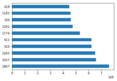

Let’s create a histogram of IMDB Scores to check the distribution of IMDB Scores across all movies. Histograms are a good way to visualize the distribution of a data set. We use the plot method on the IMDB Scores series from our movies DataFrame and pass it the argument.

movies['IMDB Score'].plot(kind="hist")
plt.show()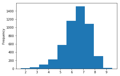

This data visualization suggests that most of the IMDB Scores fall between six and eight.

Getting statistical information about the data

Pandas has some very handy methods to look at the statistical data about our data set. For example, we can use the describe method to get a statistical summary of the data set.

movies.describe()

	Year	Duration	Aspect Ratio	Budget	Gross Earnings	Facebook Likes — Director	Facebook Likes — Actor 1	Facebook Likes — Actor 2	Facebook Likes — Actor 3	Facebook Likes — cast Total	Facebook likes — Movie	Facenumber in posters	User Votes	Reviews by Users	Reviews by Crtiics	IMDB Score
count	4935.000000	5028.000000	4714.000000	4.551000e+03	4.159000e+03	4938.000000	5035.000000	5029.000000	5020.000000	5042.000000	5042.000000	5029.000000	5.042000e+03	5022.000000	4993.000000	5042.000000
mean	2002.470517	107.201074	2.220403	3.975262e+07	4.846841e+07	686.621709	6561.323932	1652.080533	645.009761	9700.959143	7527.457160	1.371446	8.368475e+04	272.770808	140.194272	6.442007
std	12.474599	25.197441	1.385113	2.061149e+08	6.845299e+07	2813.602405	15021.977635	4042.774685	1665.041728	18165.101925	19322.070537	2.013683	1.384940e+05	377.982886	121.601675	1.125189
min	1916.000000	7.000000	1.180000	2.180000e+02	1.620000e+02	0.000000	0.000000	0.000000	0.000000	0.000000	0.000000	0.000000	5.000000e+00	1.000000	1.000000	1.600000
25%	1999.000000	93.000000	1.850000	6.000000e+06	5.340988e+06	7.000000	614.500000	281.000000	133.000000	1411.250000	0.000000	0.000000	8.599250e+03	65.000000	50.000000	5.800000
50%	2005.000000	103.000000	2.350000	2.000000e+07	2.551750e+07	49.000000	988.000000	595.000000	371.500000	3091.000000	166.000000	1.000000	3.437100e+04	156.000000	110.000000	6.600000
75%	2011.000000	118.000000	2.350000	4.500000e+07	6.230944e+07	194.750000	11000.000000	918.000000	636.000000	13758.750000	3000.000000	2.000000	9.634700e+04	326.000000	195.000000	7.200000
max	2016.000000	511.000000	16.000000	1.221550e+10	7.605058e+08	23000.000000	640000.000000	137000.000000	23000.000000	656730.000000	349000.000000	43.000000	1.689764e+06	5060.000000	813.000000	9.500000

The describe method displays below information for each of the columns.

the count or number of values
mean
standard deviation
minimum, maximum
25%, 50%, and 75% quantile

Please note that this information will be calculated only for the numeric values.

We can also use the corresponding method to access this information one at a time. For example, to get the mean of a particular column, you can use the mean method on that column.

movies["Gross Earnings"].mean()

48468407.526809327

Just like mean, there are methods available for each of the statistical information we want to access. You can read about these methods in our free pandas cheat sheet.

Reading files with no header and skipping records

Earlier in this tutorial, we saw some ways to read a particular kind of Excel file that had headers and no rows that needed skipping. Sometimes, the Excel sheet doesn’t have any header row. For such instances, you can tell pandas not to consider the first row as header or columns names. And If the Excel sheet’s first few rows contain data that should not be read in, you can ask the read_excel method to skip a certain number of rows, starting from the top.

For example, look at the top few rows of this Excel file.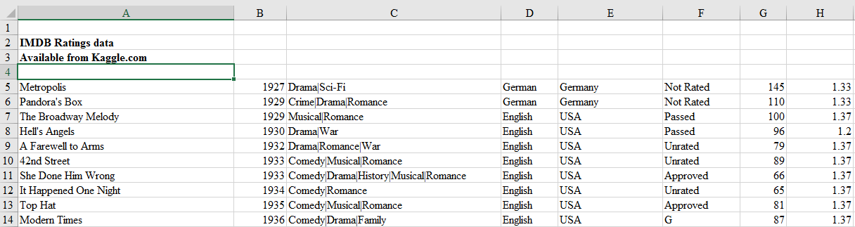

This file obviously has no header and first four rows are not actual records and hence should not be read in. We can tell read_excel there is no header by setting argument header to None and we can skip first four rows by setting argument skiprows to four.

movies_skip_rows = pd.read_excel("movies-no-header-skip-rows.xls", header=None, skiprows=4)
movies_skip_rows.head(5)

	0	1	2	3	4	5	6	7	8	9	…	15	16	17	18	19	20	21	22	23	24
0	Metropolis	1927	Drama\|Sci-Fi	German	Germany	Not Rated	145	1.33	6000000.0	26435.0	…	136	23	18.0	203	12000	1	111841	413	260.0	8.3
1	Pandora’s Box	1929	Crime\|Drama\|Romance	German	Germany	Not Rated	110	1.33	NaN	9950.0	…	426	20	3.0	455	926	1	7431	84	71.0	8.0
2	The Broadway Melody	1929	Musical\|Romance	English	USA	Passed	100	1.37	379000.0	2808000.0	…	77	28	4.0	109	167	8	4546	71	36.0	6.3
3	Hell’s Angels	1930	Drama\|War	English	USA	Passed	96	1.20	3950000.0	NaN	…	431	12	4.0	457	279	1	3753	53	35.0	7.8
4	A Farewell to Arms	1932	Drama\|Romance\|War	English	USA	Unrated	79	1.37	800000.0	NaN	…	998	164	99.0	1284	213	1	3519	46	42.0	6.6

5 rows × 25 columns

We skipped four rows from the sheet and used none of the rows as the header. Also, notice that one can combine different options in a single read statement. To skip rows at the bottom of the sheet, you can use option skip_footer, which works just like skiprows, the only difference being the rows are counted from the bottom upwards.

The column names in the previous DataFrame are numeric and were allotted as default by the pandas. We can rename the column names to descriptive ones by calling the method columns on the DataFrame and passing the column names as a list.

movies_skip_rows.columns = ['Title', 'Year', 'Genres', 'Language', 'Country', 'Content Rating', 'Duration', 'Aspect Ratio', 'Budget', 'Gross Earnings', 'Director', 'Actor 1', 'Actor 2', 'Actor 3', 'Facebook Likes - Director', 'Facebook Likes - Actor 1', 'Facebook Likes - Actor 2', 'Facebook Likes - Actor 3', 'Facebook Likes - cast Total', 'Facebook likes - Movie', 'Facenumber in posters', 'User Votes', 'Reviews by Users', 'Reviews by Crtiics', 'IMDB Score']
movies_skip_rows.head()

	Title	Year	Genres	Language	Country	Content Rating	Duration	Aspect Ratio	Budget	Gross Earnings	…	Facebook Likes — Actor 1	Facebook Likes — Actor 2	Facebook Likes — Actor 3	Facebook Likes — cast Total	Facebook likes — Movie	Facenumber in posters	User Votes	Reviews by Users	Reviews by Crtiics	IMDB Score
0	Metropolis	1927	Drama\|Sci-Fi	German	Germany	Not Rated	145	1.33	6000000.0	26435.0	…	136	23	18.0	203	12000	1	111841	413	260.0	8.3
1	Pandora’s Box	1929	Crime\|Drama\|Romance	German	Germany	Not Rated	110	1.33	NaN	9950.0	…	426	20	3.0	455	926	1	7431	84	71.0	8.0
2	The Broadway Melody	1929	Musical\|Romance	English	USA	Passed	100	1.37	379000.0	2808000.0	…	77	28	4.0	109	167	8	4546	71	36.0	6.3
3	Hell’s Angels	1930	Drama\|War	English	USA	Passed	96	1.20	3950000.0	NaN	…	431	12	4.0	457	279	1	3753	53	35.0	7.8
4	A Farewell to Arms	1932	Drama\|Romance\|War	English	USA	Unrated	79	1.37	800000.0	NaN	…	998	164	99.0	1284	213	1	3519	46	42.0	6.6

5 rows × 25 columns

Now that we have seen how to read a subset of rows from the Excel file, we can learn how to read a subset of columns.

Reading a subset of columns

Although read_excel defaults to reading and importing all columns, you can choose to import only certain columns. By passing parse_cols=6, we are telling the read_excel method to read only the first columns till index six or first seven columns (the first column being indexed zero).

movies_subset_columns = pd.read_excel(excel_file, parse_cols=6)
movies_subset_columns.head()

	Title	Year	Genres	Language	Country	Content Rating	Duration
0	Intolerance: Love’s Struggle Throughout the Ages	1916	Drama\|History\|War	NaN	USA	Not Rated	123
1	Over the Hill to the Poorhouse	1920	Crime\|Drama	NaN	USA	NaN	110
2	The Big Parade	1925	Drama\|Romance\|War	NaN	USA	Not Rated	151
3	Metropolis	1927	Drama\|Sci-Fi	German	Germany	Not Rated	145
4	Pandora’s Box	1929	Crime\|Drama\|Romance	German	Germany	Not Rated	110

Alternatively, you can pass in a list of numbers, which will let you import columns at particular indexes.

Applying formulas on the columns

One of the much-used features of Excel is to apply formulas to create new columns from existing column values. In our Excel file, we have Gross Earnings and Budget columns. We can get Net earnings by subtracting Budget from Gross earnings. We could then apply this formula in the Excel file to all the rows. We can do this in pandas also as shown below.

movies["Net Earnings"] = movies["Gross Earnings"] - movies["Budget"]

Above, we used pandas to create a new column called Net Earnings, and populated it with the difference of Gross Earnings and Budget. It’s worth noting the difference here in how formulas are treated in Excel versus pandas. In Excel, a formula lives in the cell and updates when the data changes — with Python, the calculations happen and the values are stored — if Gross Earnings for one movie was manually changed, Net Earnings won’t be updated.

Let’s use the sort_values method to sort the data by the new column we created and visualize the top 10 movies by Net Earnings.

sorted_movies = movies[['Net Earnings']].sort_values(['Net Earnings'], ascending=[False])sorted_movies.head(10)['Net Earnings'].plot.barh()
plt.show()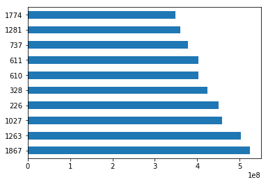

Pivot Table in pandas

Advanced Excel users also often use pivot tables. A pivot table summarizes the data of another table by grouping the data on an index and applying operations such as sorting, summing, or averaging. You can use this feature in pandas too.

We need to first identify the column or columns that will serve as the index, and the column(s) on which the summarizing formula will be applied. Let’s start small, by choosing Year as the index column and Gross Earnings as the summarization column and creating a separate DataFrame from this data.

movies_subset = movies[['Year', 'Gross Earnings']]
movies_subset.head()

	Year	Gross Earnings
0	1916.0	NaN
1	1920.0	3000000.0
2	1925.0	NaN
3	1927.0	26435.0
4	1929.0	9950.0

We now call pivot_table on this subset of data. The method pivot_table takes a parameter index. As mentioned, we want to use Year as the index.

earnings_by_year = movies_subset.pivot_table(index=['Year'])
earnings_by_year.head()

	Gross Earnings
Year
1916.0	NaN
1920.0	3000000.0
1925.0	NaN
1927.0	26435.0
1929.0	1408975.0

This gave us a pivot table with grouping on Year and summarization on the sum of Gross Earnings. Notice, we didn’t need to specify Gross Earnings column explicitly as pandas automatically identified it the values on which summarization should be applied.

We can use this pivot table to create some data visualizations. We can call the plot method on the DataFrame to create a line plot and call the show method to display the plot in the notebook.

earnings_by_year.plot()
plt.show()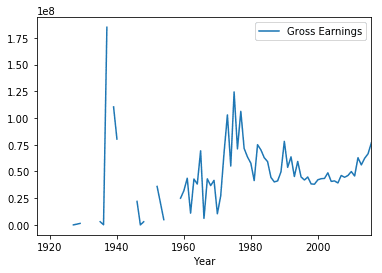

We saw how to pivot with a single column as the index. Things will get more interesting if we can use multiple columns. Let’s create another DataFrame subset but this time we will choose the columns, Country, Language and Gross Earnings.

movies_subset = movies[['Country', 'Language', 'Gross Earnings']]
movies_subset.head()

	Country	Language	Gross Earnings
0	USA	NaN	NaN
1	USA	NaN	3000000.0
2	USA	NaN	NaN
3	Germany	German	26435.0
4	Germany	German	9950.0

We will use columns Country and Language as the index for the pivot table. We will use Gross Earnings as summarization table, however, we do not need to specify this explicitly as we saw earlier.

earnings_by_co_lang = movies_subset.pivot_table(index=['Country', 'Language'])
earnings_by_co_lang.head()

		Gross Earnings
Country	Language
Afghanistan	Dari	1.127331e+06
Argentina	Spanish	7.230936e+06
Aruba	English	1.007614e+07
Australia	Aboriginal	6.165429e+06
Dzongkha	5.052950e+05

Let’s visualize this pivot table with a bar plot. Since there are still few hundred records in this pivot table, we will plot just a few of them.

earnings_by_co_lang.head(20).plot(kind='bar', figsize=(20,8))
plt.show()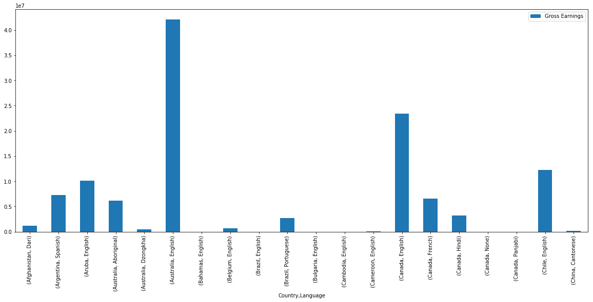

Exporting the results to Excel

If you’re going to be working with colleagues who use Excel, saving Excel files out of pandas is important. You can export or write a pandas DataFrame to an Excel file using pandas to_excel method. Pandas uses the xlwt Python module internally for writing to Excel files. The to_excel method is called on the DataFrame we want to export.We also need to pass a filename to which this DataFrame will be written.

movies.to_excel('output.xlsx')

By default, the index is also saved to the output file. However, sometimes the index doesn’t provide any useful information. For example, the movies DataFrame has a numeric auto-increment index, that was not part of the original Excel data.

movies.head()

	Title	Year	Genres	Language	Country	Content Rating	Duration	Aspect Ratio	Budget	Gross Earnings	…	Facebook Likes — Actor 2	Facebook Likes — Actor 3	Facebook Likes — cast Total	Facebook likes — Movie	Facenumber in posters	User Votes	Reviews by Users	Reviews by Crtiics	IMDB Score	Net Earnings
0	Intolerance: Love’s Struggle Throughout the Ages	1916.0	Drama\|History\|War	NaN	USA	Not Rated	123.0	1.33	385907.0	NaN	…	22.0	9.0	481	691	1.0	10718	88.0	69.0	8.0	NaN
1	Over the Hill to the Poorhouse	1920.0	Crime\|Drama	NaN	USA	NaN	110.0	1.33	100000.0	3000000.0	…	2.0	0.0	4	0	1.0	5	1.0	1.0	4.8	2900000.0
2	The Big Parade	1925.0	Drama\|Romance\|War	NaN	USA	Not Rated	151.0	1.33	245000.0	NaN	…	12.0	6.0	108	226	0.0	4849	45.0	48.0	8.3	NaN
3	Metropolis	1927.0	Drama\|Sci-Fi	German	Germany	Not Rated	145.0	1.33	6000000.0	26435.0	…	23.0	18.0	203	12000	1.0	111841	413.0	260.0	8.3	-5973565.0
4	Pandora’s Box	1929.0	Crime\|Drama\|Romance	German	Germany	Not Rated	110.0	1.33	NaN	9950.0	…	20.0	3.0	455	926	1.0	7431	84.0	71.0	8.0	NaN

5 rows × 26 columns

You can choose to skip the index by passing along index-False.

movies.to_excel('output.xlsx', index=False)

We need to be able to make our output files look nice before we can send it out to our co-workers. We can use pandas ExcelWriter class along with the XlsxWriter Python module to apply the formatting.

We can do use these advanced output options by creating a ExcelWriter object and use this object to write to the EXcel file.

writer = pd.ExcelWriter('output.xlsx', engine='xlsxwriter')
movies.to_excel(writer, index=False, sheet_name='report')
workbook = writer.bookworksheet = writer.sheets['report']

We can apply customizations by calling add_format on the workbook we are writing to. Here we are setting header format as bold.

header_fmt = workbook.add_format({'bold': True})
worksheet.set_row(0, None, header_fmt)

Finally, we save the output file by calling the method save on the writer object.

writer.save()

As an example, we saved the data with column headers set as bold. And the saved file looks like the image below.

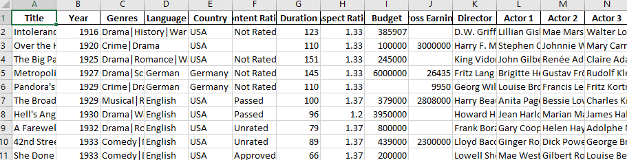
Like this, one can use XlsxWriter to apply various formatting to the output Excel file.

Conclusion

Pandas is not a replacement for Excel. Both tools have their place in the data analysis workflow and can be very great companion tools. As we demonstrated, pandas can do a lot of complex data analysis and manipulations, which depending on your need and expertise, can go beyond what you can achieve if you are just using Excel. One of the major benefits of using Python and pandas over Excel is that it helps you automate Excel file processing by writing scripts and integrating with your automated data workflow. Pandas also has excellent methods for reading all kinds of data from Excel files. You can export your results from pandas back to Excel too if that’s preferred by your intended audience.

On the other hand, Excel is a such a widely used data tool, it’s not a wise to ignore it. Acquiring expertise in both pandas and Excel and making them work together gives you skills that can help you stand out in your organization.

If you’d like to learn more about this topic, check out Dataquest’s interactive Pandas and NumPy Fundamentals course, and our Data Analyst in Python, and Data Scientist in Python paths that will help you become job-ready in around 6 months.

Источник

Watch Now This tutorial has a related video course created by the Real Python team. Watch it together with the written tutorial to deepen your understanding: Reading and Writing Files With Pandas

pandas is a powerful and flexible Python package that allows you to work with labeled and time series data. It also provides statistics methods, enables plotting, and more. One crucial feature of pandas is its ability to write and read Excel, CSV, and many other types of files. Functions like the pandas read_csv() method enable you to work with files effectively. You can use them to save the data and labels from pandas objects to a file and load them later as pandas Series or DataFrame instances.

In this tutorial, you’ll learn:

What the pandas IO tools API is
How to read and write data to and from files
How to work with various file formats
How to work with big data efficiently

Let’s start reading and writing files!

Installing pandas

The code in this tutorial is executed with CPython 3.7.4 and pandas 0.25.1. It would be beneficial to make sure you have the latest versions of Python and pandas on your machine. You might want to create a new virtual environment and install the dependencies for this tutorial.

First, you’ll need the pandas library. You may already have it installed. If you don’t, then you can install it with pip:

Once the installation process completes, you should have pandas installed and ready.

Anaconda is an excellent Python distribution that comes with Python, many useful packages like pandas, and a package and environment manager called Conda. To learn more about Anaconda, check out Setting Up Python for Machine Learning on Windows.

If you don’t have pandas in your virtual environment, then you can install it with Conda:

Conda is powerful as it manages the dependencies and their versions. To learn more about working with Conda, you can check out the official documentation.

Preparing Data

In this tutorial, you’ll use the data related to 20 countries. Here’s an overview of the data and sources you’ll be working with:

Country is denoted by the country name. Each country is in the top 10 list for either population, area, or gross domestic product (GDP). The row labels for the dataset are the three-letter country codes defined in ISO 3166-1. The column label for the dataset is COUNTRY.
Population is expressed in millions. The data comes from a list of countries and dependencies by population on Wikipedia. The column label for the dataset is POP.
Area is expressed in thousands of kilometers squared. The data comes from a list of countries and dependencies by area on Wikipedia. The column label for the dataset is AREA.
Gross domestic product is expressed in millions of U.S. dollars, according to the United Nations data for 2017. You can find this data in the list of countries by nominal GDP on Wikipedia. The column label for the dataset is GDP.
Continent is either Africa, Asia, Oceania, Europe, North America, or South America. You can find this information on Wikipedia as well. The column label for the dataset is CONT.
Independence day is a date that commemorates a nation’s independence. The data comes from the list of national independence days on Wikipedia. The dates are shown in ISO 8601 format. The first four digits represent the year, the next two numbers are the month, and the last two are for the day of the month. The column label for the dataset is IND_DAY.

This is how the data looks as a table:

	COUNTRY	POP	AREA	GDP	CONT	IND_DAY
CHN	China	1398.72	9596.96	12234.78	Asia
IND	India	1351.16	3287.26	2575.67	Asia	1947-08-15
USA	US	329.74	9833.52	19485.39	N.America	1776-07-04
IDN	Indonesia	268.07	1910.93	1015.54	Asia	1945-08-17
BRA	Brazil	210.32	8515.77	2055.51	S.America	1822-09-07
PAK	Pakistan	205.71	881.91	302.14	Asia	1947-08-14
NGA	Nigeria	200.96	923.77	375.77	Africa	1960-10-01
BGD	Bangladesh	167.09	147.57	245.63	Asia	1971-03-26
RUS	Russia	146.79	17098.25	1530.75		1992-06-12
MEX	Mexico	126.58	1964.38	1158.23	N.America	1810-09-16
JPN	Japan	126.22	377.97	4872.42	Asia
DEU	Germany	83.02	357.11	3693.20	Europe
FRA	France	67.02	640.68	2582.49	Europe	1789-07-14
GBR	UK	66.44	242.50	2631.23	Europe
ITA	Italy	60.36	301.34	1943.84	Europe
ARG	Argentina	44.94	2780.40	637.49	S.America	1816-07-09
DZA	Algeria	43.38	2381.74	167.56	Africa	1962-07-05
CAN	Canada	37.59	9984.67	1647.12	N.America	1867-07-01
AUS	Australia	25.47	7692.02	1408.68	Oceania
KAZ	Kazakhstan	18.53	2724.90	159.41	Asia	1991-12-16

You may notice that some of the data is missing. For example, the continent for Russia is not specified because it spreads across both Europe and Asia. There are also several missing independence days because the data source omits them.

You can organize this data in Python using a nested dictionary:

data = {
    'CHN': {'COUNTRY': 'China', 'POP': 1_398.72, 'AREA': 9_596.96,
            'GDP': 12_234.78, 'CONT': 'Asia'},
    'IND': {'COUNTRY': 'India', 'POP': 1_351.16, 'AREA': 3_287.26,
            'GDP': 2_575.67, 'CONT': 'Asia', 'IND_DAY': '1947-08-15'},
    'USA': {'COUNTRY': 'US', 'POP': 329.74, 'AREA': 9_833.52,
            'GDP': 19_485.39, 'CONT': 'N.America',
            'IND_DAY': '1776-07-04'},
    'IDN': {'COUNTRY': 'Indonesia', 'POP': 268.07, 'AREA': 1_910.93,
            'GDP': 1_015.54, 'CONT': 'Asia', 'IND_DAY': '1945-08-17'},
    'BRA': {'COUNTRY': 'Brazil', 'POP': 210.32, 'AREA': 8_515.77,
            'GDP': 2_055.51, 'CONT': 'S.America', 'IND_DAY': '1822-09-07'},
    'PAK': {'COUNTRY': 'Pakistan', 'POP': 205.71, 'AREA': 881.91,
            'GDP': 302.14, 'CONT': 'Asia', 'IND_DAY': '1947-08-14'},
    'NGA': {'COUNTRY': 'Nigeria', 'POP': 200.96, 'AREA': 923.77,
            'GDP': 375.77, 'CONT': 'Africa', 'IND_DAY': '1960-10-01'},
    'BGD': {'COUNTRY': 'Bangladesh', 'POP': 167.09, 'AREA': 147.57,
            'GDP': 245.63, 'CONT': 'Asia', 'IND_DAY': '1971-03-26'},
    'RUS': {'COUNTRY': 'Russia', 'POP': 146.79, 'AREA': 17_098.25,
            'GDP': 1_530.75, 'IND_DAY': '1992-06-12'},
    'MEX': {'COUNTRY': 'Mexico', 'POP': 126.58, 'AREA': 1_964.38,
            'GDP': 1_158.23, 'CONT': 'N.America', 'IND_DAY': '1810-09-16'},
    'JPN': {'COUNTRY': 'Japan', 'POP': 126.22, 'AREA': 377.97,
            'GDP': 4_872.42, 'CONT': 'Asia'},
    'DEU': {'COUNTRY': 'Germany', 'POP': 83.02, 'AREA': 357.11,
            'GDP': 3_693.20, 'CONT': 'Europe'},
    'FRA': {'COUNTRY': 'France', 'POP': 67.02, 'AREA': 640.68,
            'GDP': 2_582.49, 'CONT': 'Europe', 'IND_DAY': '1789-07-14'},
    'GBR': {'COUNTRY': 'UK', 'POP': 66.44, 'AREA': 242.50,
            'GDP': 2_631.23, 'CONT': 'Europe'},
    'ITA': {'COUNTRY': 'Italy', 'POP': 60.36, 'AREA': 301.34,
            'GDP': 1_943.84, 'CONT': 'Europe'},
    'ARG': {'COUNTRY': 'Argentina', 'POP': 44.94, 'AREA': 2_780.40,
            'GDP': 637.49, 'CONT': 'S.America', 'IND_DAY': '1816-07-09'},
    'DZA': {'COUNTRY': 'Algeria', 'POP': 43.38, 'AREA': 2_381.74,
            'GDP': 167.56, 'CONT': 'Africa', 'IND_DAY': '1962-07-05'},
    'CAN': {'COUNTRY': 'Canada', 'POP': 37.59, 'AREA': 9_984.67,
            'GDP': 1_647.12, 'CONT': 'N.America', 'IND_DAY': '1867-07-01'},
    'AUS': {'COUNTRY': 'Australia', 'POP': 25.47, 'AREA': 7_692.02,
            'GDP': 1_408.68, 'CONT': 'Oceania'},
    'KAZ': {'COUNTRY': 'Kazakhstan', 'POP': 18.53, 'AREA': 2_724.90,
            'GDP': 159.41, 'CONT': 'Asia', 'IND_DAY': '1991-12-16'}
}

columns = ('COUNTRY', 'POP', 'AREA', 'GDP', 'CONT', 'IND_DAY')

Each row of the table is written as an inner dictionary whose keys are the column names and values are the corresponding data. These dictionaries are then collected as the values in the outer data dictionary. The corresponding keys for data are the three-letter country codes.

You can use this data to create an instance of a pandas DataFrame. First, you need to import pandas:

>>>

>>> import pandas as pd

Now that you have pandas imported, you can use the DataFrame constructor and data to create a DataFrame object.

data is organized in such a way that the country codes correspond to columns. You can reverse the rows and columns of a DataFrame with the property .T:

>>>

>>> df = pd.DataFrame(data=data).T
>>> df
        COUNTRY      POP     AREA      GDP       CONT     IND_DAY
CHN       China  1398.72  9596.96  12234.8       Asia         NaN
IND       India  1351.16  3287.26  2575.67       Asia  1947-08-15
USA          US   329.74  9833.52  19485.4  N.America  1776-07-04
IDN   Indonesia   268.07  1910.93  1015.54       Asia  1945-08-17
BRA      Brazil   210.32  8515.77  2055.51  S.America  1822-09-07
PAK    Pakistan   205.71   881.91   302.14       Asia  1947-08-14
NGA     Nigeria   200.96   923.77   375.77     Africa  1960-10-01
BGD  Bangladesh   167.09   147.57   245.63       Asia  1971-03-26
RUS      Russia   146.79  17098.2  1530.75        NaN  1992-06-12
MEX      Mexico   126.58  1964.38  1158.23  N.America  1810-09-16
JPN       Japan   126.22   377.97  4872.42       Asia         NaN
DEU     Germany    83.02   357.11   3693.2     Europe         NaN
FRA      France    67.02   640.68  2582.49     Europe  1789-07-14
GBR          UK    66.44    242.5  2631.23     Europe         NaN
ITA       Italy    60.36   301.34  1943.84     Europe         NaN
ARG   Argentina    44.94   2780.4   637.49  S.America  1816-07-09
DZA     Algeria    43.38  2381.74   167.56     Africa  1962-07-05
CAN      Canada    37.59  9984.67  1647.12  N.America  1867-07-01
AUS   Australia    25.47  7692.02  1408.68    Oceania         NaN
KAZ  Kazakhstan    18.53   2724.9   159.41       Asia  1991-12-16

Now you have your DataFrame object populated with the data about each country.

Versions of Python older than 3.6 did not guarantee the order of keys in dictionaries. To ensure the order of columns is maintained for older versions of Python and pandas, you can specify index=columns:

>>>

>>> df = pd.DataFrame(data=data, index=columns).T

Now that you’ve prepared your data, you’re ready to start working with files!

Using the pandas `read_csv()` and `.to_csv()` Functions

A comma-separated values (CSV) file is a plaintext file with a .csv extension that holds tabular data. This is one of the most popular file formats for storing large amounts of data. Each row of the CSV file represents a single table row. The values in the same row are by default separated with commas, but you could change the separator to a semicolon, tab, space, or some other character.

Write a CSV File

You can save your pandas DataFrame as a CSV file with .to_csv():

>>>

>>> df.to_csv('data.csv')

That’s it! You’ve created the file data.csv in your current working directory. You can expand the code block below to see how your CSV file should look:

,COUNTRY,POP,AREA,GDP,CONT,IND_DAY
CHN,China,1398.72,9596.96,12234.78,Asia,
IND,India,1351.16,3287.26,2575.67,Asia,1947-08-15
USA,US,329.74,9833.52,19485.39,N.America,1776-07-04
IDN,Indonesia,268.07,1910.93,1015.54,Asia,1945-08-17
BRA,Brazil,210.32,8515.77,2055.51,S.America,1822-09-07
PAK,Pakistan,205.71,881.91,302.14,Asia,1947-08-14
NGA,Nigeria,200.96,923.77,375.77,Africa,1960-10-01
BGD,Bangladesh,167.09,147.57,245.63,Asia,1971-03-26
RUS,Russia,146.79,17098.25,1530.75,,1992-06-12
MEX,Mexico,126.58,1964.38,1158.23,N.America,1810-09-16
JPN,Japan,126.22,377.97,4872.42,Asia,
DEU,Germany,83.02,357.11,3693.2,Europe,
FRA,France,67.02,640.68,2582.49,Europe,1789-07-14
GBR,UK,66.44,242.5,2631.23,Europe,
ITA,Italy,60.36,301.34,1943.84,Europe,
ARG,Argentina,44.94,2780.4,637.49,S.America,1816-07-09
DZA,Algeria,43.38,2381.74,167.56,Africa,1962-07-05
CAN,Canada,37.59,9984.67,1647.12,N.America,1867-07-01
AUS,Australia,25.47,7692.02,1408.68,Oceania,
KAZ,Kazakhstan,18.53,2724.9,159.41,Asia,1991-12-16

This text file contains the data separated with commas. The first column contains the row labels. In some cases, you’ll find them irrelevant. If you don’t want to keep them, then you can pass the argument index=False to .to_csv().

Read a CSV File

Once your data is saved in a CSV file, you’ll likely want to load and use it from time to time. You can do that with the pandas read_csv() function:

>>>

>>> df = pd.read_csv('data.csv', index_col=0)
>>> df
        COUNTRY      POP      AREA       GDP       CONT     IND_DAY
CHN       China  1398.72   9596.96  12234.78       Asia         NaN
IND       India  1351.16   3287.26   2575.67       Asia  1947-08-15
USA          US   329.74   9833.52  19485.39  N.America  1776-07-04
IDN   Indonesia   268.07   1910.93   1015.54       Asia  1945-08-17
BRA      Brazil   210.32   8515.77   2055.51  S.America  1822-09-07
PAK    Pakistan   205.71    881.91    302.14       Asia  1947-08-14
NGA     Nigeria   200.96    923.77    375.77     Africa  1960-10-01
BGD  Bangladesh   167.09    147.57    245.63       Asia  1971-03-26
RUS      Russia   146.79  17098.25   1530.75        NaN  1992-06-12
MEX      Mexico   126.58   1964.38   1158.23  N.America  1810-09-16
JPN       Japan   126.22    377.97   4872.42       Asia         NaN
DEU     Germany    83.02    357.11   3693.20     Europe         NaN
FRA      France    67.02    640.68   2582.49     Europe  1789-07-14
GBR          UK    66.44    242.50   2631.23     Europe         NaN
ITA       Italy    60.36    301.34   1943.84     Europe         NaN
ARG   Argentina    44.94   2780.40    637.49  S.America  1816-07-09
DZA     Algeria    43.38   2381.74    167.56     Africa  1962-07-05
CAN      Canada    37.59   9984.67   1647.12  N.America  1867-07-01
AUS   Australia    25.47   7692.02   1408.68    Oceania         NaN
KAZ  Kazakhstan    18.53   2724.90    159.41       Asia  1991-12-16

In this case, the pandas read_csv() function returns a new DataFrame with the data and labels from the file data.csv, which you specified with the first argument. This string can be any valid path, including URLs.

The parameter index_col specifies the column from the CSV file that contains the row labels. You assign a zero-based column index to this parameter. You should determine the value of index_col when the CSV file contains the row labels to avoid loading them as data.

You’ll learn more about using pandas with CSV files later on in this tutorial. You can also check out Reading and Writing CSV Files in Python to see how to handle CSV files with the built-in Python library csv as well.

Using pandas to Write and Read Excel Files

Microsoft Excel is probably the most widely-used spreadsheet software. While older versions used binary .xls files, Excel 2007 introduced the new XML-based .xlsx file. You can read and write Excel files in pandas, similar to CSV files. However, you’ll need to install the following Python packages first:

xlwt to write to .xls files
openpyxl or XlsxWriter to write to .xlsx files
xlrd to read Excel files

You can install them using pip with a single command:

$ pip install xlwt openpyxl xlsxwriter xlrd

You can also use Conda:

$ conda install xlwt openpyxl xlsxwriter xlrd

Please note that you don’t have to install all these packages. For example, you don’t need both openpyxl and XlsxWriter. If you’re going to work just with .xls files, then you don’t need any of them! However, if you intend to work only with .xlsx files, then you’re going to need at least one of them, but not xlwt. Take some time to decide which packages are right for your project.

Write an Excel File

Once you have those packages installed, you can save your DataFrame in an Excel file with .to_excel():

>>>

>>> df.to_excel('data.xlsx')

The argument 'data.xlsx' represents the target file and, optionally, its path. The above statement should create the file data.xlsx in your current working directory. That file should look like this:

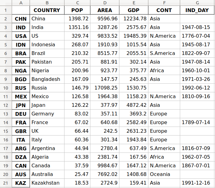
The first column of the file contains the labels of the rows, while the other columns store data.

Read an Excel File

You can load data from Excel files with read_excel():

>>>

>>> df = pd.read_excel('data.xlsx', index_col=0)
>>> df
        COUNTRY      POP      AREA       GDP       CONT     IND_DAY
CHN       China  1398.72   9596.96  12234.78       Asia         NaN
IND       India  1351.16   3287.26   2575.67       Asia  1947-08-15
USA          US   329.74   9833.52  19485.39  N.America  1776-07-04
IDN   Indonesia   268.07   1910.93   1015.54       Asia  1945-08-17
BRA      Brazil   210.32   8515.77   2055.51  S.America  1822-09-07
PAK    Pakistan   205.71    881.91    302.14       Asia  1947-08-14
NGA     Nigeria   200.96    923.77    375.77     Africa  1960-10-01
BGD  Bangladesh   167.09    147.57    245.63       Asia  1971-03-26
RUS      Russia   146.79  17098.25   1530.75        NaN  1992-06-12
MEX      Mexico   126.58   1964.38   1158.23  N.America  1810-09-16
JPN       Japan   126.22    377.97   4872.42       Asia         NaN
DEU     Germany    83.02    357.11   3693.20     Europe         NaN
FRA      France    67.02    640.68   2582.49     Europe  1789-07-14
GBR          UK    66.44    242.50   2631.23     Europe         NaN
ITA       Italy    60.36    301.34   1943.84     Europe         NaN
ARG   Argentina    44.94   2780.40    637.49  S.America  1816-07-09
DZA     Algeria    43.38   2381.74    167.56     Africa  1962-07-05
CAN      Canada    37.59   9984.67   1647.12  N.America  1867-07-01
AUS   Australia    25.47   7692.02   1408.68    Oceania         NaN
KAZ  Kazakhstan    18.53   2724.90    159.41       Asia  1991-12-16

read_excel() returns a new DataFrame that contains the values from data.xlsx. You can also use read_excel() with OpenDocument spreadsheets, or .ods files.

You’ll learn more about working with Excel files later on in this tutorial. You can also check out Using pandas to Read Large Excel Files in Python.

Understanding the pandas IO API

pandas IO Tools is the API that allows you to save the contents of Series and DataFrame objects to the clipboard, objects, or files of various types. It also enables loading data from the clipboard, objects, or files.

Write Files

Series and DataFrame objects have methods that enable writing data and labels to the clipboard or files. They’re named with the pattern .to_<file-type>(), where <file-type> is the type of the target file.

You’ve learned about .to_csv() and .to_excel(), but there are others, including:

.to_json()
.to_html()
.to_sql()
.to_pickle()

There are still more file types that you can write to, so this list is not exhaustive.

These methods have parameters specifying the target file path where you saved the data and labels. This is mandatory in some cases and optional in others. If this option is available and you choose to omit it, then the methods return the objects (like strings or iterables) with the contents of DataFrame instances.

The optional parameter compression decides how to compress the file with the data and labels. You’ll learn more about it later on. There are a few other parameters, but they’re mostly specific to one or several methods. You won’t go into them in detail here.

Read Files

pandas functions for reading the contents of files are named using the pattern .read_<file-type>(), where <file-type> indicates the type of the file to read. You’ve already seen the pandas read_csv() and read_excel() functions. Here are a few others:

read_json()
read_html()
read_sql()
read_pickle()

These functions have a parameter that specifies the target file path. It can be any valid string that represents the path, either on a local machine or in a URL. Other objects are also acceptable depending on the file type.

The optional parameter compression determines the type of decompression to use for the compressed files. You’ll learn about it later on in this tutorial. There are other parameters, but they’re specific to one or several functions. You won’t go into them in detail here.

Working With Different File Types

The pandas library offers a wide range of possibilities for saving your data to files and loading data from files. In this section, you’ll learn more about working with CSV and Excel files. You’ll also see how to use other types of files, like JSON, web pages, databases, and Python pickle files.

CSV Files

You’ve already learned how to read and write CSV files. Now let’s dig a little deeper into the details. When you use .to_csv() to save your DataFrame, you can provide an argument for the parameter path_or_buf to specify the path, name, and extension of the target file.

path_or_buf is the first argument .to_csv() will get. It can be any string that represents a valid file path that includes the file name and its extension. You’ve seen this in a previous example. However, if you omit path_or_buf, then .to_csv() won’t create any files. Instead, it’ll return the corresponding string:

>>>

>>> df = pd.DataFrame(data=data).T
>>> s = df.to_csv()
>>> print(s)
,COUNTRY,POP,AREA,GDP,CONT,IND_DAY
CHN,China,1398.72,9596.96,12234.78,Asia,
IND,India,1351.16,3287.26,2575.67,Asia,1947-08-15
USA,US,329.74,9833.52,19485.39,N.America,1776-07-04
IDN,Indonesia,268.07,1910.93,1015.54,Asia,1945-08-17
BRA,Brazil,210.32,8515.77,2055.51,S.America,1822-09-07
PAK,Pakistan,205.71,881.91,302.14,Asia,1947-08-14
NGA,Nigeria,200.96,923.77,375.77,Africa,1960-10-01
BGD,Bangladesh,167.09,147.57,245.63,Asia,1971-03-26
RUS,Russia,146.79,17098.25,1530.75,,1992-06-12
MEX,Mexico,126.58,1964.38,1158.23,N.America,1810-09-16
JPN,Japan,126.22,377.97,4872.42,Asia,
DEU,Germany,83.02,357.11,3693.2,Europe,
FRA,France,67.02,640.68,2582.49,Europe,1789-07-14
GBR,UK,66.44,242.5,2631.23,Europe,
ITA,Italy,60.36,301.34,1943.84,Europe,
ARG,Argentina,44.94,2780.4,637.49,S.America,1816-07-09
DZA,Algeria,43.38,2381.74,167.56,Africa,1962-07-05
CAN,Canada,37.59,9984.67,1647.12,N.America,1867-07-01
AUS,Australia,25.47,7692.02,1408.68,Oceania,
KAZ,Kazakhstan,18.53,2724.9,159.41,Asia,1991-12-16

Now you have the string s instead of a CSV file. You also have some missing values in your DataFrame object. For example, the continent for Russia and the independence days for several countries (China, Japan, and so on) are not available. In data science and machine learning, you must handle missing values carefully. pandas excels here! By default, pandas uses the NaN value to replace the missing values.

The continent that corresponds to Russia in df is nan:

>>>

>>> df.loc['RUS', 'CONT']
nan

This example uses .loc[] to get data with the specified row and column names.

When you save your DataFrame to a CSV file, empty strings ('') will represent the missing data. You can see this both in your file data.csv and in the string s. If you want to change this behavior, then use the optional parameter na_rep:

>>>

>>> df.to_csv('new-data.csv', na_rep='(missing)')

This code produces the file new-data.csv where the missing values are no longer empty strings. You can expand the code block below to see how this file should look:

,COUNTRY,POP,AREA,GDP,CONT,IND_DAY
CHN,China,1398.72,9596.96,12234.78,Asia,(missing)
IND,India,1351.16,3287.26,2575.67,Asia,1947-08-15
USA,US,329.74,9833.52,19485.39,N.America,1776-07-04
IDN,Indonesia,268.07,1910.93,1015.54,Asia,1945-08-17
BRA,Brazil,210.32,8515.77,2055.51,S.America,1822-09-07
PAK,Pakistan,205.71,881.91,302.14,Asia,1947-08-14
NGA,Nigeria,200.96,923.77,375.77,Africa,1960-10-01
BGD,Bangladesh,167.09,147.57,245.63,Asia,1971-03-26
RUS,Russia,146.79,17098.25,1530.75,(missing),1992-06-12
MEX,Mexico,126.58,1964.38,1158.23,N.America,1810-09-16
JPN,Japan,126.22,377.97,4872.42,Asia,(missing)
DEU,Germany,83.02,357.11,3693.2,Europe,(missing)
FRA,France,67.02,640.68,2582.49,Europe,1789-07-14
GBR,UK,66.44,242.5,2631.23,Europe,(missing)
ITA,Italy,60.36,301.34,1943.84,Europe,(missing)
ARG,Argentina,44.94,2780.4,637.49,S.America,1816-07-09
DZA,Algeria,43.38,2381.74,167.56,Africa,1962-07-05
CAN,Canada,37.59,9984.67,1647.12,N.America,1867-07-01
AUS,Australia,25.47,7692.02,1408.68,Oceania,(missing)
KAZ,Kazakhstan,18.53,2724.9,159.41,Asia,1991-12-16

Now, the string '(missing)' in the file corresponds to the nan values from df.

When pandas reads files, it considers the empty string ('') and a few others as missing values by default:

'nan'
'-nan'
'NA'
'N/A'
'NaN'
'null'

If you don’t want this behavior, then you can pass keep_default_na=False to the pandas read_csv() function. To specify other labels for missing values, use the parameter na_values:

>>>

>>> pd.read_csv('new-data.csv', index_col=0, na_values='(missing)')
        COUNTRY      POP      AREA       GDP       CONT     IND_DAY
CHN       China  1398.72   9596.96  12234.78       Asia         NaN
IND       India  1351.16   3287.26   2575.67       Asia  1947-08-15
USA          US   329.74   9833.52  19485.39  N.America  1776-07-04
IDN   Indonesia   268.07   1910.93   1015.54       Asia  1945-08-17
BRA      Brazil   210.32   8515.77   2055.51  S.America  1822-09-07
PAK    Pakistan   205.71    881.91    302.14       Asia  1947-08-14
NGA     Nigeria   200.96    923.77    375.77     Africa  1960-10-01
BGD  Bangladesh   167.09    147.57    245.63       Asia  1971-03-26
RUS      Russia   146.79  17098.25   1530.75        NaN  1992-06-12
MEX      Mexico   126.58   1964.38   1158.23  N.America  1810-09-16
JPN       Japan   126.22    377.97   4872.42       Asia         NaN
DEU     Germany    83.02    357.11   3693.20     Europe         NaN
FRA      France    67.02    640.68   2582.49     Europe  1789-07-14
GBR          UK    66.44    242.50   2631.23     Europe         NaN
ITA       Italy    60.36    301.34   1943.84     Europe         NaN
ARG   Argentina    44.94   2780.40    637.49  S.America  1816-07-09
DZA     Algeria    43.38   2381.74    167.56     Africa  1962-07-05
CAN      Canada    37.59   9984.67   1647.12  N.America  1867-07-01
AUS   Australia    25.47   7692.02   1408.68    Oceania         NaN
KAZ  Kazakhstan    18.53   2724.90    159.41       Asia  1991-12-16

Here, you’ve marked the string '(missing)' as a new missing data label, and pandas replaced it with nan when it read the file.

When you load data from a file, pandas assigns the data types to the values of each column by default. You can check these types with .dtypes:

>>>

>>> df = pd.read_csv('data.csv', index_col=0)
>>> df.dtypes
COUNTRY     object
POP        float64
AREA       float64
GDP        float64
CONT        object
IND_DAY     object
dtype: object

The columns with strings and dates ('COUNTRY', 'CONT', and 'IND_DAY') have the data type object. Meanwhile, the numeric columns contain 64-bit floating-point numbers (float64).

You can use the parameter dtype to specify the desired data types and parse_dates to force use of datetimes:

>>>

>>> dtypes = {'POP': 'float32', 'AREA': 'float32', 'GDP': 'float32'}
>>> df = pd.read_csv('data.csv', index_col=0, dtype=dtypes,
...                  parse_dates=['IND_DAY'])
>>> df.dtypes
COUNTRY            object
POP               float32
AREA              float32
GDP               float32
CONT               object
IND_DAY    datetime64[ns]
dtype: object
>>> df['IND_DAY']
CHN          NaT
IND   1947-08-15
USA   1776-07-04
IDN   1945-08-17
BRA   1822-09-07
PAK   1947-08-14
NGA   1960-10-01
BGD   1971-03-26
RUS   1992-06-12
MEX   1810-09-16
JPN          NaT
DEU          NaT
FRA   1789-07-14
GBR          NaT
ITA          NaT
ARG   1816-07-09
DZA   1962-07-05
CAN   1867-07-01
AUS          NaT
KAZ   1991-12-16
Name: IND_DAY, dtype: datetime64[ns]

Now, you have 32-bit floating-point numbers (float32) as specified with dtype. These differ slightly from the original 64-bit numbers because of smaller precision. The values in the last column are considered as dates and have the data type datetime64. That’s why the NaN values in this column are replaced with NaT.

Now that you have real dates, you can save them in the format you like:

>>>

>>> df = pd.read_csv('data.csv', index_col=0, parse_dates=['IND_DAY'])
>>> df.to_csv('formatted-data.csv', date_format='%B %d, %Y')

Here, you’ve specified the parameter date_format to be '%B %d, %Y'. You can expand the code block below to see the resulting file:

,COUNTRY,POP,AREA,GDP,CONT,IND_DAY
CHN,China,1398.72,9596.96,12234.78,Asia,
IND,India,1351.16,3287.26,2575.67,Asia,"August 15, 1947"
USA,US,329.74,9833.52,19485.39,N.America,"July 04, 1776"
IDN,Indonesia,268.07,1910.93,1015.54,Asia,"August 17, 1945"
BRA,Brazil,210.32,8515.77,2055.51,S.America,"September 07, 1822"
PAK,Pakistan,205.71,881.91,302.14,Asia,"August 14, 1947"
NGA,Nigeria,200.96,923.77,375.77,Africa,"October 01, 1960"
BGD,Bangladesh,167.09,147.57,245.63,Asia,"March 26, 1971"
RUS,Russia,146.79,17098.25,1530.75,,"June 12, 1992"
MEX,Mexico,126.58,1964.38,1158.23,N.America,"September 16, 1810"
JPN,Japan,126.22,377.97,4872.42,Asia,
DEU,Germany,83.02,357.11,3693.2,Europe,
FRA,France,67.02,640.68,2582.49,Europe,"July 14, 1789"
GBR,UK,66.44,242.5,2631.23,Europe,
ITA,Italy,60.36,301.34,1943.84,Europe,
ARG,Argentina,44.94,2780.4,637.49,S.America,"July 09, 1816"
DZA,Algeria,43.38,2381.74,167.56,Africa,"July 05, 1962"
CAN,Canada,37.59,9984.67,1647.12,N.America,"July 01, 1867"
AUS,Australia,25.47,7692.02,1408.68,Oceania,
KAZ,Kazakhstan,18.53,2724.9,159.41,Asia,"December 16, 1991"

The format of the dates is different now. The format '%B %d, %Y' means the date will first display the full name of the month, then the day followed by a comma, and finally the full year.

There are several other optional parameters that you can use with .to_csv():

sep denotes a values separator.
decimal indicates a decimal separator.
encoding sets the file encoding.
header specifies whether you want to write column labels in the file.

Here’s how you would pass arguments for sep and header:

>>>

>>> s = df.to_csv(sep=';', header=False)
>>> print(s)
CHN;China;1398.72;9596.96;12234.78;Asia;
IND;India;1351.16;3287.26;2575.67;Asia;1947-08-15
USA;US;329.74;9833.52;19485.39;N.America;1776-07-04
IDN;Indonesia;268.07;1910.93;1015.54;Asia;1945-08-17
BRA;Brazil;210.32;8515.77;2055.51;S.America;1822-09-07
PAK;Pakistan;205.71;881.91;302.14;Asia;1947-08-14
NGA;Nigeria;200.96;923.77;375.77;Africa;1960-10-01
BGD;Bangladesh;167.09;147.57;245.63;Asia;1971-03-26
RUS;Russia;146.79;17098.25;1530.75;;1992-06-12
MEX;Mexico;126.58;1964.38;1158.23;N.America;1810-09-16
JPN;Japan;126.22;377.97;4872.42;Asia;
DEU;Germany;83.02;357.11;3693.2;Europe;
FRA;France;67.02;640.68;2582.49;Europe;1789-07-14
GBR;UK;66.44;242.5;2631.23;Europe;
ITA;Italy;60.36;301.34;1943.84;Europe;
ARG;Argentina;44.94;2780.4;637.49;S.America;1816-07-09
DZA;Algeria;43.38;2381.74;167.56;Africa;1962-07-05
CAN;Canada;37.59;9984.67;1647.12;N.America;1867-07-01
AUS;Australia;25.47;7692.02;1408.68;Oceania;
KAZ;Kazakhstan;18.53;2724.9;159.41;Asia;1991-12-16

The data is separated with a semicolon (';') because you’ve specified sep=';'. Also, since you passed header=False, you see your data without the header row of column names.

The pandas read_csv() function has many additional options for managing missing data, working with dates and times, quoting, encoding, handling errors, and more. For instance, if you have a file with one data column and want to get a Series object instead of a DataFrame, then you can pass squeeze=True to read_csv(). You’ll learn later on about data compression and decompression, as well as how to skip rows and columns.

JSON Files

JSON stands for JavaScript object notation. JSON files are plaintext files used for data interchange, and humans can read them easily. They follow the ISO/IEC 21778:2017 and ECMA-404 standards and use the .json extension. Python and pandas work well with JSON files, as Python’s json library offers built-in support for them.

You can save the data from your DataFrame to a JSON file with .to_json(). Start by creating a DataFrame object again. Use the dictionary data that holds the data about countries and then apply .to_json():

>>>

>>> df = pd.DataFrame(data=data).T
>>> df.to_json('data-columns.json')

This code produces the file data-columns.json. You can expand the code block below to see how this file should look:

{"COUNTRY":{"CHN":"China","IND":"India","USA":"US","IDN":"Indonesia","BRA":"Brazil","PAK":"Pakistan","NGA":"Nigeria","BGD":"Bangladesh","RUS":"Russia","MEX":"Mexico","JPN":"Japan","DEU":"Germany","FRA":"France","GBR":"UK","ITA":"Italy","ARG":"Argentina","DZA":"Algeria","CAN":"Canada","AUS":"Australia","KAZ":"Kazakhstan"},"POP":{"CHN":1398.72,"IND":1351.16,"USA":329.74,"IDN":268.07,"BRA":210.32,"PAK":205.71,"NGA":200.96,"BGD":167.09,"RUS":146.79,"MEX":126.58,"JPN":126.22,"DEU":83.02,"FRA":67.02,"GBR":66.44,"ITA":60.36,"ARG":44.94,"DZA":43.38,"CAN":37.59,"AUS":25.47,"KAZ":18.53},"AREA":{"CHN":9596.96,"IND":3287.26,"USA":9833.52,"IDN":1910.93,"BRA":8515.77,"PAK":881.91,"NGA":923.77,"BGD":147.57,"RUS":17098.25,"MEX":1964.38,"JPN":377.97,"DEU":357.11,"FRA":640.68,"GBR":242.5,"ITA":301.34,"ARG":2780.4,"DZA":2381.74,"CAN":9984.67,"AUS":7692.02,"KAZ":2724.9},"GDP":{"CHN":12234.78,"IND":2575.67,"USA":19485.39,"IDN":1015.54,"BRA":2055.51,"PAK":302.14,"NGA":375.77,"BGD":245.63,"RUS":1530.75,"MEX":1158.23,"JPN":4872.42,"DEU":3693.2,"FRA":2582.49,"GBR":2631.23,"ITA":1943.84,"ARG":637.49,"DZA":167.56,"CAN":1647.12,"AUS":1408.68,"KAZ":159.41},"CONT":{"CHN":"Asia","IND":"Asia","USA":"N.America","IDN":"Asia","BRA":"S.America","PAK":"Asia","NGA":"Africa","BGD":"Asia","RUS":null,"MEX":"N.America","JPN":"Asia","DEU":"Europe","FRA":"Europe","GBR":"Europe","ITA":"Europe","ARG":"S.America","DZA":"Africa","CAN":"N.America","AUS":"Oceania","KAZ":"Asia"},"IND_DAY":{"CHN":null,"IND":"1947-08-15","USA":"1776-07-04","IDN":"1945-08-17","BRA":"1822-09-07","PAK":"1947-08-14","NGA":"1960-10-01","BGD":"1971-03-26","RUS":"1992-06-12","MEX":"1810-09-16","JPN":null,"DEU":null,"FRA":"1789-07-14","GBR":null,"ITA":null,"ARG":"1816-07-09","DZA":"1962-07-05","CAN":"1867-07-01","AUS":null,"KAZ":"1991-12-16"}}

data-columns.json has one large dictionary with the column labels as keys and the corresponding inner dictionaries as values.

You can get a different file structure if you pass an argument for the optional parameter orient:

>>>

>>> df.to_json('data-index.json', orient='index')

The orient parameter defaults to 'columns'. Here, you’ve set it to index.

You should get a new file data-index.json. You can expand the code block below to see the changes:

{"CHN":{"COUNTRY":"China","POP":1398.72,"AREA":9596.96,"GDP":12234.78,"CONT":"Asia","IND_DAY":null},"IND":{"COUNTRY":"India","POP":1351.16,"AREA":3287.26,"GDP":2575.67,"CONT":"Asia","IND_DAY":"1947-08-15"},"USA":{"COUNTRY":"US","POP":329.74,"AREA":9833.52,"GDP":19485.39,"CONT":"N.America","IND_DAY":"1776-07-04"},"IDN":{"COUNTRY":"Indonesia","POP":268.07,"AREA":1910.93,"GDP":1015.54,"CONT":"Asia","IND_DAY":"1945-08-17"},"BRA":{"COUNTRY":"Brazil","POP":210.32,"AREA":8515.77,"GDP":2055.51,"CONT":"S.America","IND_DAY":"1822-09-07"},"PAK":{"COUNTRY":"Pakistan","POP":205.71,"AREA":881.91,"GDP":302.14,"CONT":"Asia","IND_DAY":"1947-08-14"},"NGA":{"COUNTRY":"Nigeria","POP":200.96,"AREA":923.77,"GDP":375.77,"CONT":"Africa","IND_DAY":"1960-10-01"},"BGD":{"COUNTRY":"Bangladesh","POP":167.09,"AREA":147.57,"GDP":245.63,"CONT":"Asia","IND_DAY":"1971-03-26"},"RUS":{"COUNTRY":"Russia","POP":146.79,"AREA":17098.25,"GDP":1530.75,"CONT":null,"IND_DAY":"1992-06-12"},"MEX":{"COUNTRY":"Mexico","POP":126.58,"AREA":1964.38,"GDP":1158.23,"CONT":"N.America","IND_DAY":"1810-09-16"},"JPN":{"COUNTRY":"Japan","POP":126.22,"AREA":377.97,"GDP":4872.42,"CONT":"Asia","IND_DAY":null},"DEU":{"COUNTRY":"Germany","POP":83.02,"AREA":357.11,"GDP":3693.2,"CONT":"Europe","IND_DAY":null},"FRA":{"COUNTRY":"France","POP":67.02,"AREA":640.68,"GDP":2582.49,"CONT":"Europe","IND_DAY":"1789-07-14"},"GBR":{"COUNTRY":"UK","POP":66.44,"AREA":242.5,"GDP":2631.23,"CONT":"Europe","IND_DAY":null},"ITA":{"COUNTRY":"Italy","POP":60.36,"AREA":301.34,"GDP":1943.84,"CONT":"Europe","IND_DAY":null},"ARG":{"COUNTRY":"Argentina","POP":44.94,"AREA":2780.4,"GDP":637.49,"CONT":"S.America","IND_DAY":"1816-07-09"},"DZA":{"COUNTRY":"Algeria","POP":43.38,"AREA":2381.74,"GDP":167.56,"CONT":"Africa","IND_DAY":"1962-07-05"},"CAN":{"COUNTRY":"Canada","POP":37.59,"AREA":9984.67,"GDP":1647.12,"CONT":"N.America","IND_DAY":"1867-07-01"},"AUS":{"COUNTRY":"Australia","POP":25.47,"AREA":7692.02,"GDP":1408.68,"CONT":"Oceania","IND_DAY":null},"KAZ":{"COUNTRY":"Kazakhstan","POP":18.53,"AREA":2724.9,"GDP":159.41,"CONT":"Asia","IND_DAY":"1991-12-16"}}

data-index.json also has one large dictionary, but this time the row labels are the keys, and the inner dictionaries are the values.

There are few more options for orient. One of them is 'records':

>>>

>>> df.to_json('data-records.json', orient='records')

This code should yield the file data-records.json. You can expand the code block below to see the content:

[{"COUNTRY":"China","POP":1398.72,"AREA":9596.96,"GDP":12234.78,"CONT":"Asia","IND_DAY":null},{"COUNTRY":"India","POP":1351.16,"AREA":3287.26,"GDP":2575.67,"CONT":"Asia","IND_DAY":"1947-08-15"},{"COUNTRY":"US","POP":329.74,"AREA":9833.52,"GDP":19485.39,"CONT":"N.America","IND_DAY":"1776-07-04"},{"COUNTRY":"Indonesia","POP":268.07,"AREA":1910.93,"GDP":1015.54,"CONT":"Asia","IND_DAY":"1945-08-17"},{"COUNTRY":"Brazil","POP":210.32,"AREA":8515.77,"GDP":2055.51,"CONT":"S.America","IND_DAY":"1822-09-07"},{"COUNTRY":"Pakistan","POP":205.71,"AREA":881.91,"GDP":302.14,"CONT":"Asia","IND_DAY":"1947-08-14"},{"COUNTRY":"Nigeria","POP":200.96,"AREA":923.77,"GDP":375.77,"CONT":"Africa","IND_DAY":"1960-10-01"},{"COUNTRY":"Bangladesh","POP":167.09,"AREA":147.57,"GDP":245.63,"CONT":"Asia","IND_DAY":"1971-03-26"},{"COUNTRY":"Russia","POP":146.79,"AREA":17098.25,"GDP":1530.75,"CONT":null,"IND_DAY":"1992-06-12"},{"COUNTRY":"Mexico","POP":126.58,"AREA":1964.38,"GDP":1158.23,"CONT":"N.America","IND_DAY":"1810-09-16"},{"COUNTRY":"Japan","POP":126.22,"AREA":377.97,"GDP":4872.42,"CONT":"Asia","IND_DAY":null},{"COUNTRY":"Germany","POP":83.02,"AREA":357.11,"GDP":3693.2,"CONT":"Europe","IND_DAY":null},{"COUNTRY":"France","POP":67.02,"AREA":640.68,"GDP":2582.49,"CONT":"Europe","IND_DAY":"1789-07-14"},{"COUNTRY":"UK","POP":66.44,"AREA":242.5,"GDP":2631.23,"CONT":"Europe","IND_DAY":null},{"COUNTRY":"Italy","POP":60.36,"AREA":301.34,"GDP":1943.84,"CONT":"Europe","IND_DAY":null},{"COUNTRY":"Argentina","POP":44.94,"AREA":2780.4,"GDP":637.49,"CONT":"S.America","IND_DAY":"1816-07-09"},{"COUNTRY":"Algeria","POP":43.38,"AREA":2381.74,"GDP":167.56,"CONT":"Africa","IND_DAY":"1962-07-05"},{"COUNTRY":"Canada","POP":37.59,"AREA":9984.67,"GDP":1647.12,"CONT":"N.America","IND_DAY":"1867-07-01"},{"COUNTRY":"Australia","POP":25.47,"AREA":7692.02,"GDP":1408.68,"CONT":"Oceania","IND_DAY":null},{"COUNTRY":"Kazakhstan","POP":18.53,"AREA":2724.9,"GDP":159.41,"CONT":"Asia","IND_DAY":"1991-12-16"}]

data-records.json holds a list with one dictionary for each row. The row labels are not written.

You can get another interesting file structure with orient='split':

>>>

>>> df.to_json('data-split.json', orient='split')

The resulting file is data-split.json. You can expand the code block below to see how this file should look:

{"columns":["COUNTRY","POP","AREA","GDP","CONT","IND_DAY"],"index":["CHN","IND","USA","IDN","BRA","PAK","NGA","BGD","RUS","MEX","JPN","DEU","FRA","GBR","ITA","ARG","DZA","CAN","AUS","KAZ"],"data":[["China",1398.72,9596.96,12234.78,"Asia",null],["India",1351.16,3287.26,2575.67,"Asia","1947-08-15"],["US",329.74,9833.52,19485.39,"N.America","1776-07-04"],["Indonesia",268.07,1910.93,1015.54,"Asia","1945-08-17"],["Brazil",210.32,8515.77,2055.51,"S.America","1822-09-07"],["Pakistan",205.71,881.91,302.14,"Asia","1947-08-14"],["Nigeria",200.96,923.77,375.77,"Africa","1960-10-01"],["Bangladesh",167.09,147.57,245.63,"Asia","1971-03-26"],["Russia",146.79,17098.25,1530.75,null,"1992-06-12"],["Mexico",126.58,1964.38,1158.23,"N.America","1810-09-16"],["Japan",126.22,377.97,4872.42,"Asia",null],["Germany",83.02,357.11,3693.2,"Europe",null],["France",67.02,640.68,2582.49,"Europe","1789-07-14"],["UK",66.44,242.5,2631.23,"Europe",null],["Italy",60.36,301.34,1943.84,"Europe",null],["Argentina",44.94,2780.4,637.49,"S.America","1816-07-09"],["Algeria",43.38,2381.74,167.56,"Africa","1962-07-05"],["Canada",37.59,9984.67,1647.12,"N.America","1867-07-01"],["Australia",25.47,7692.02,1408.68,"Oceania",null],["Kazakhstan",18.53,2724.9,159.41,"Asia","1991-12-16"]]}

data-split.json contains one dictionary that holds the following lists:

The names of the columns
The labels of the rows
The inner lists (two-dimensional sequence) that hold data values

If you don’t provide the value for the optional parameter path_or_buf that defines the file path, then .to_json() will return a JSON string instead of writing the results to a file. This behavior is consistent with .to_csv().

There are other optional parameters you can use. For instance, you can set index=False to forgo saving row labels. You can manipulate precision with double_precision, and dates with date_format and date_unit. These last two parameters are particularly important when you have time series among your data:

>>>

>>> df = pd.DataFrame(data=data).T
>>> df['IND_DAY'] = pd.to_datetime(df['IND_DAY'])
>>> df.dtypes
COUNTRY            object
POP                object
AREA               object
GDP                object
CONT               object
IND_DAY    datetime64[ns]
dtype: object

>>> df.to_json('data-time.json')

In this example, you’ve created the DataFrame from the dictionary data and used to_datetime() to convert the values in the last column to datetime64. You can expand the code block below to see the resulting file:

{"COUNTRY":{"CHN":"China","IND":"India","USA":"US","IDN":"Indonesia","BRA":"Brazil","PAK":"Pakistan","NGA":"Nigeria","BGD":"Bangladesh","RUS":"Russia","MEX":"Mexico","JPN":"Japan","DEU":"Germany","FRA":"France","GBR":"UK","ITA":"Italy","ARG":"Argentina","DZA":"Algeria","CAN":"Canada","AUS":"Australia","KAZ":"Kazakhstan"},"POP":{"CHN":1398.72,"IND":1351.16,"USA":329.74,"IDN":268.07,"BRA":210.32,"PAK":205.71,"NGA":200.96,"BGD":167.09,"RUS":146.79,"MEX":126.58,"JPN":126.22,"DEU":83.02,"FRA":67.02,"GBR":66.44,"ITA":60.36,"ARG":44.94,"DZA":43.38,"CAN":37.59,"AUS":25.47,"KAZ":18.53},"AREA":{"CHN":9596.96,"IND":3287.26,"USA":9833.52,"IDN":1910.93,"BRA":8515.77,"PAK":881.91,"NGA":923.77,"BGD":147.57,"RUS":17098.25,"MEX":1964.38,"JPN":377.97,"DEU":357.11,"FRA":640.68,"GBR":242.5,"ITA":301.34,"ARG":2780.4,"DZA":2381.74,"CAN":9984.67,"AUS":7692.02,"KAZ":2724.9},"GDP":{"CHN":12234.78,"IND":2575.67,"USA":19485.39,"IDN":1015.54,"BRA":2055.51,"PAK":302.14,"NGA":375.77,"BGD":245.63,"RUS":1530.75,"MEX":1158.23,"JPN":4872.42,"DEU":3693.2,"FRA":2582.49,"GBR":2631.23,"ITA":1943.84,"ARG":637.49,"DZA":167.56,"CAN":1647.12,"AUS":1408.68,"KAZ":159.41},"CONT":{"CHN":"Asia","IND":"Asia","USA":"N.America","IDN":"Asia","BRA":"S.America","PAK":"Asia","NGA":"Africa","BGD":"Asia","RUS":null,"MEX":"N.America","JPN":"Asia","DEU":"Europe","FRA":"Europe","GBR":"Europe","ITA":"Europe","ARG":"S.America","DZA":"Africa","CAN":"N.America","AUS":"Oceania","KAZ":"Asia"},"IND_DAY":{"CHN":null,"IND":-706320000000,"USA":-6106060800000,"IDN":-769219200000,"BRA":-4648924800000,"PAK":-706406400000,"NGA":-291945600000,"BGD":38793600000,"RUS":708307200000,"MEX":-5026838400000,"JPN":null,"DEU":null,"FRA":-5694969600000,"GBR":null,"ITA":null,"ARG":-4843411200000,"DZA":-236476800000,"CAN":-3234729600000,"AUS":null,"KAZ":692841600000}}

In this file, you have large integers instead of dates for the independence days. That’s because the default value of the optional parameter date_format is 'epoch' whenever orient isn’t 'table'. This default behavior expresses dates as an epoch in milliseconds relative to midnight on January 1, 1970.

However, if you pass date_format='iso', then you’ll get the dates in the ISO 8601 format. In addition, date_unit decides the units of time:

>>>

>>> df = pd.DataFrame(data=data).T
>>> df['IND_DAY'] = pd.to_datetime(df['IND_DAY'])
>>> df.to_json('new-data-time.json', date_format='iso', date_unit='s')

This code produces the following JSON file:

{"COUNTRY":{"CHN":"China","IND":"India","USA":"US","IDN":"Indonesia","BRA":"Brazil","PAK":"Pakistan","NGA":"Nigeria","BGD":"Bangladesh","RUS":"Russia","MEX":"Mexico","JPN":"Japan","DEU":"Germany","FRA":"France","GBR":"UK","ITA":"Italy","ARG":"Argentina","DZA":"Algeria","CAN":"Canada","AUS":"Australia","KAZ":"Kazakhstan"},"POP":{"CHN":1398.72,"IND":1351.16,"USA":329.74,"IDN":268.07,"BRA":210.32,"PAK":205.71,"NGA":200.96,"BGD":167.09,"RUS":146.79,"MEX":126.58,"JPN":126.22,"DEU":83.02,"FRA":67.02,"GBR":66.44,"ITA":60.36,"ARG":44.94,"DZA":43.38,"CAN":37.59,"AUS":25.47,"KAZ":18.53},"AREA":{"CHN":9596.96,"IND":3287.26,"USA":9833.52,"IDN":1910.93,"BRA":8515.77,"PAK":881.91,"NGA":923.77,"BGD":147.57,"RUS":17098.25,"MEX":1964.38,"JPN":377.97,"DEU":357.11,"FRA":640.68,"GBR":242.5,"ITA":301.34,"ARG":2780.4,"DZA":2381.74,"CAN":9984.67,"AUS":7692.02,"KAZ":2724.9},"GDP":{"CHN":12234.78,"IND":2575.67,"USA":19485.39,"IDN":1015.54,"BRA":2055.51,"PAK":302.14,"NGA":375.77,"BGD":245.63,"RUS":1530.75,"MEX":1158.23,"JPN":4872.42,"DEU":3693.2,"FRA":2582.49,"GBR":2631.23,"ITA":1943.84,"ARG":637.49,"DZA":167.56,"CAN":1647.12,"AUS":1408.68,"KAZ":159.41},"CONT":{"CHN":"Asia","IND":"Asia","USA":"N.America","IDN":"Asia","BRA":"S.America","PAK":"Asia","NGA":"Africa","BGD":"Asia","RUS":null,"MEX":"N.America","JPN":"Asia","DEU":"Europe","FRA":"Europe","GBR":"Europe","ITA":"Europe","ARG":"S.America","DZA":"Africa","CAN":"N.America","AUS":"Oceania","KAZ":"Asia"},"IND_DAY":{"CHN":null,"IND":"1947-08-15T00:00:00Z","USA":"1776-07-04T00:00:00Z","IDN":"1945-08-17T00:00:00Z","BRA":"1822-09-07T00:00:00Z","PAK":"1947-08-14T00:00:00Z","NGA":"1960-10-01T00:00:00Z","BGD":"1971-03-26T00:00:00Z","RUS":"1992-06-12T00:00:00Z","MEX":"1810-09-16T00:00:00Z","JPN":null,"DEU":null,"FRA":"1789-07-14T00:00:00Z","GBR":null,"ITA":null,"ARG":"1816-07-09T00:00:00Z","DZA":"1962-07-05T00:00:00Z","CAN":"1867-07-01T00:00:00Z","AUS":null,"KAZ":"1991-12-16T00:00:00Z"}}

The dates in the resulting file are in the ISO 8601 format.

You can load the data from a JSON file with read_json():

>>>

>>> df = pd.read_json('data-index.json', orient='index',
...                   convert_dates=['IND_DAY'])

The parameter convert_dates has a similar purpose as parse_dates when you use it to read CSV files. The optional parameter orient is very important because it specifies how pandas understands the structure of the file.

There are other optional parameters you can use as well:

Set the encoding with encoding.
Manipulate dates with convert_dates and keep_default_dates.
Impact precision with dtype and precise_float.
Decode numeric data directly to NumPy arrays with numpy=True.

Note that you might lose the order of rows and columns when using the JSON format to store your data.

HTML Files

An HTML is a plaintext file that uses hypertext markup language to help browsers render web pages. The extensions for HTML files are .html and .htm. You’ll need to install an HTML parser library like lxml or html5lib to be able to work with HTML files:

$pip install lxml html5lib

You can also use Conda to install the same packages:

$ conda install lxml html5lib

Once you have these libraries, you can save the contents of your DataFrame as an HTML file with .to_html():

>>>

df = pd.DataFrame(data=data).T
df.to_html('data.html')

This code generates a file data.html. You can expand the code block below to see how this file should look:

<table border="1" class="dataframe">
  <thead>
    <tr style="text-align: right;">
      <th></th>
      <th>COUNTRY</th>
      <th>POP</th>
      <th>AREA</th>
      <th>GDP</th>
      <th>CONT</th>
      <th>IND_DAY</th>
    </tr>
  </thead>
  <tbody>
    <tr>
      <th>CHN</th>
      <td>China</td>
      <td>1398.72</td>
      <td>9596.96</td>
      <td>12234.8</td>
      <td>Asia</td>
      <td>NaN</td>
    </tr>
    <tr>
      <th>IND</th>
      <td>India</td>
      <td>1351.16</td>
      <td>3287.26</td>
      <td>2575.67</td>
      <td>Asia</td>
      <td>1947-08-15</td>
    </tr>
    <tr>
      <th>USA</th>
      <td>US</td>
      <td>329.74</td>
      <td>9833.52</td>
      <td>19485.4</td>
      <td>N.America</td>
      <td>1776-07-04</td>
    </tr>
    <tr>
      <th>IDN</th>
      <td>Indonesia</td>
      <td>268.07</td>
      <td>1910.93</td>
      <td>1015.54</td>
      <td>Asia</td>
      <td>1945-08-17</td>
    </tr>
    <tr>
      <th>BRA</th>
      <td>Brazil</td>
      <td>210.32</td>
      <td>8515.77</td>
      <td>2055.51</td>
      <td>S.America</td>
      <td>1822-09-07</td>
    </tr>
    <tr>
      <th>PAK</th>
      <td>Pakistan</td>
      <td>205.71</td>
      <td>881.91</td>
      <td>302.14</td>
      <td>Asia</td>
      <td>1947-08-14</td>
    </tr>
    <tr>
      <th>NGA</th>
      <td>Nigeria</td>
      <td>200.96</td>
      <td>923.77</td>
      <td>375.77</td>
      <td>Africa</td>
      <td>1960-10-01</td>
    </tr>
    <tr>
      <th>BGD</th>
      <td>Bangladesh</td>
      <td>167.09</td>
      <td>147.57</td>
      <td>245.63</td>
      <td>Asia</td>
      <td>1971-03-26</td>
    </tr>
    <tr>
      <th>RUS</th>
      <td>Russia</td>
      <td>146.79</td>
      <td>17098.2</td>
      <td>1530.75</td>
      <td>NaN</td>
      <td>1992-06-12</td>
    </tr>
    <tr>
      <th>MEX</th>
      <td>Mexico</td>
      <td>126.58</td>
      <td>1964.38</td>
      <td>1158.23</td>
      <td>N.America</td>
      <td>1810-09-16</td>
    </tr>
    <tr>
      <th>JPN</th>
      <td>Japan</td>
      <td>126.22</td>
      <td>377.97</td>
      <td>4872.42</td>
      <td>Asia</td>
      <td>NaN</td>
    </tr>
    <tr>
      <th>DEU</th>
      <td>Germany</td>
      <td>83.02</td>
      <td>357.11</td>
      <td>3693.2</td>
      <td>Europe</td>
      <td>NaN</td>
    </tr>
    <tr>
      <th>FRA</th>
      <td>France</td>
      <td>67.02</td>
      <td>640.68</td>
      <td>2582.49</td>
      <td>Europe</td>
      <td>1789-07-14</td>
    </tr>
    <tr>
      <th>GBR</th>
      <td>UK</td>
      <td>66.44</td>
      <td>242.5</td>
      <td>2631.23</td>
      <td>Europe</td>
      <td>NaN</td>
    </tr>
    <tr>
      <th>ITA</th>
      <td>Italy</td>
      <td>60.36</td>
      <td>301.34</td>
      <td>1943.84</td>
      <td>Europe</td>
      <td>NaN</td>
    </tr>
    <tr>
      <th>ARG</th>
      <td>Argentina</td>
      <td>44.94</td>
      <td>2780.4</td>
      <td>637.49</td>
      <td>S.America</td>
      <td>1816-07-09</td>
    </tr>
    <tr>
      <th>DZA</th>
      <td>Algeria</td>
      <td>43.38</td>
      <td>2381.74</td>
      <td>167.56</td>
      <td>Africa</td>
      <td>1962-07-05</td>
    </tr>
    <tr>
      <th>CAN</th>
      <td>Canada</td>
      <td>37.59</td>
      <td>9984.67</td>
      <td>1647.12</td>
      <td>N.America</td>
      <td>1867-07-01</td>
    </tr>
    <tr>
      <th>AUS</th>
      <td>Australia</td>
      <td>25.47</td>
      <td>7692.02</td>
      <td>1408.68</td>
      <td>Oceania</td>
      <td>NaN</td>
    </tr>
    <tr>
      <th>KAZ</th>
      <td>Kazakhstan</td>
      <td>18.53</td>
      <td>2724.9</td>
      <td>159.41</td>
      <td>Asia</td>
      <td>1991-12-16</td>
    </tr>
  </tbody>
</table>

This file shows the DataFrame contents nicely. However, notice that you haven’t obtained an entire web page. You’ve just output the data that corresponds to df in the HTML format.

.to_html() won’t create a file if you don’t provide the optional parameter buf, which denotes the buffer to write to. If you leave this parameter out, then your code will return a string as it did with .to_csv() and .to_json().

Here are some other optional parameters:

header determines whether to save the column names.
index determines whether to save the row labels.
classes assigns cascading style sheet (CSS) classes.
render_links specifies whether to convert URLs to HTML links.
table_id assigns the CSS id to the table tag.
escape decides whether to convert the characters <, >, and & to HTML-safe strings.

You use parameters like these to specify different aspects of the resulting files or strings.

You can create a DataFrame object from a suitable HTML file using read_html(), which will return a DataFrame instance or a list of them:

>>>

>>> df = pd.read_html('data.html', index_col=0, parse_dates=['IND_DAY'])

This is very similar to what you did when reading CSV files. You also have parameters that help you work with dates, missing values, precision, encoding, HTML parsers, and more.

Excel Files

You’ve already learned how to read and write Excel files with pandas. However, there are a few more options worth considering. For one, when you use .to_excel(), you can specify the name of the target worksheet with the optional parameter sheet_name:

>>>

>>> df = pd.DataFrame(data=data).T
>>> df.to_excel('data.xlsx', sheet_name='COUNTRIES')

Here, you create a file data.xlsx with a worksheet called COUNTRIES that stores the data. The string 'data.xlsx' is the argument for the parameter excel_writer that defines the name of the Excel file or its path.

The optional parameters startrow and startcol both default to 0 and indicate the upper left-most cell where the data should start being written:

>>>

>>> df.to_excel('data-shifted.xlsx', sheet_name='COUNTRIES',
...             startrow=2, startcol=4)

Here, you specify that the table should start in the third row and the fifth column. You also used zero-based indexing, so the third row is denoted by 2 and the fifth column by 4.

Now the resulting worksheet looks like this:

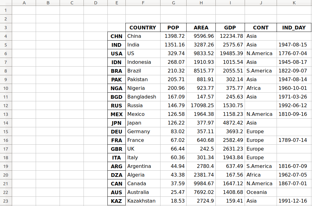
As you can see, the table starts in the third row 2 and the fifth column E.

.read_excel() also has the optional parameter sheet_name that specifies which worksheets to read when loading data. It can take on one of the following values:

The zero-based index of the worksheet
The name of the worksheet
The list of indices or names to read multiple sheets
The value None to read all sheets

Here’s how you would use this parameter in your code:

>>>

>>> df = pd.read_excel('data.xlsx', sheet_name=0, index_col=0,
...                    parse_dates=['IND_DAY'])
>>> df = pd.read_excel('data.xlsx', sheet_name='COUNTRIES', index_col=0,
...                    parse_dates=['IND_DAY'])

Both statements above create the same DataFrame because the sheet_name parameters have the same values. In both cases, sheet_name=0 and sheet_name='COUNTRIES' refer to the same worksheet. The argument parse_dates=['IND_DAY'] tells pandas to try to consider the values in this column as dates or times.

There are other optional parameters you can use with .read_excel() and .to_excel() to determine the Excel engine, the encoding, the way to handle missing values and infinities, the method for writing column names and row labels, and so on.

SQL Files

pandas IO tools can also read and write databases. In this next example, you’ll write your data to a database called data.db. To get started, you’ll need the SQLAlchemy package. To learn more about it, you can read the official ORM tutorial. You’ll also need the database driver. Python has a built-in driver for SQLite.

You can install SQLAlchemy with pip:

You can also install it with Conda:

$ conda install sqlalchemy

Once you have SQLAlchemy installed, import create_engine() and create a database engine:

>>>

>>> from sqlalchemy import create_engine
>>> engine = create_engine('sqlite:///data.db', echo=False)

Now that you have everything set up, the next step is to create a DataFrame object. It’s convenient to specify the data types and apply .to_sql().

>>>

>>> dtypes = {'POP': 'float64', 'AREA': 'float64', 'GDP': 'float64',
...           'IND_DAY': 'datetime64'}
>>> df = pd.DataFrame(data=data).T.astype(dtype=dtypes)
>>> df.dtypes
COUNTRY            object
POP               float64
AREA              float64
GDP               float64
CONT               object
IND_DAY    datetime64[ns]
dtype: object

.astype() is a very convenient method you can use to set multiple data types at once.

Once you’ve created your DataFrame, you can save it to the database with .to_sql():

>>>

>>> df.to_sql('data.db', con=engine, index_label='ID')

The parameter con is used to specify the database connection or engine that you want to use. The optional parameter index_label specifies how to call the database column with the row labels. You’ll often see it take on the value ID, Id, or id.

You should get the database data.db with a single table that looks like this:

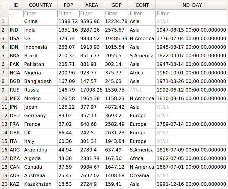
The first column contains the row labels. To omit writing them into the database, pass index=False to .to_sql(). The other columns correspond to the columns of the DataFrame.

There are a few more optional parameters. For example, you can use schema to specify the database schema and dtype to determine the types of the database columns. You can also use if_exists, which says what to do if a database with the same name and path already exists:

if_exists='fail' raises a ValueError and is the default.
if_exists='replace' drops the table and inserts new values.
if_exists='append' inserts new values into the table.

You can load the data from the database with read_sql():

>>>

>>> df = pd.read_sql('data.db', con=engine, index_col='ID')
>>> df
        COUNTRY      POP      AREA       GDP       CONT    IND_DAY
ID
CHN       China  1398.72   9596.96  12234.78       Asia        NaT
IND       India  1351.16   3287.26   2575.67       Asia 1947-08-15
USA          US   329.74   9833.52  19485.39  N.America 1776-07-04
IDN   Indonesia   268.07   1910.93   1015.54       Asia 1945-08-17
BRA      Brazil   210.32   8515.77   2055.51  S.America 1822-09-07
PAK    Pakistan   205.71    881.91    302.14       Asia 1947-08-14
NGA     Nigeria   200.96    923.77    375.77     Africa 1960-10-01
BGD  Bangladesh   167.09    147.57    245.63       Asia 1971-03-26
RUS      Russia   146.79  17098.25   1530.75       None 1992-06-12
MEX      Mexico   126.58   1964.38   1158.23  N.America 1810-09-16
JPN       Japan   126.22    377.97   4872.42       Asia        NaT
DEU     Germany    83.02    357.11   3693.20     Europe        NaT
FRA      France    67.02    640.68   2582.49     Europe 1789-07-14
GBR          UK    66.44    242.50   2631.23     Europe        NaT
ITA       Italy    60.36    301.34   1943.84     Europe        NaT
ARG   Argentina    44.94   2780.40    637.49  S.America 1816-07-09
DZA     Algeria    43.38   2381.74    167.56     Africa 1962-07-05
CAN      Canada    37.59   9984.67   1647.12  N.America 1867-07-01
AUS   Australia    25.47   7692.02   1408.68    Oceania        NaT
KAZ  Kazakhstan    18.53   2724.90    159.41       Asia 1991-12-16

The parameter index_col specifies the name of the column with the row labels. Note that this inserts an extra row after the header that starts with ID. You can fix this behavior with the following line of code:

>>>

>>> df.index.name = None
>>> df
        COUNTRY      POP      AREA       GDP       CONT    IND_DAY
CHN       China  1398.72   9596.96  12234.78       Asia        NaT
IND       India  1351.16   3287.26   2575.67       Asia 1947-08-15
USA          US   329.74   9833.52  19485.39  N.America 1776-07-04
IDN   Indonesia   268.07   1910.93   1015.54       Asia 1945-08-17
BRA      Brazil   210.32   8515.77   2055.51  S.America 1822-09-07
PAK    Pakistan   205.71    881.91    302.14       Asia 1947-08-14
NGA     Nigeria   200.96    923.77    375.77     Africa 1960-10-01
BGD  Bangladesh   167.09    147.57    245.63       Asia 1971-03-26
RUS      Russia   146.79  17098.25   1530.75       None 1992-06-12
MEX      Mexico   126.58   1964.38   1158.23  N.America 1810-09-16
JPN       Japan   126.22    377.97   4872.42       Asia        NaT
DEU     Germany    83.02    357.11   3693.20     Europe        NaT
FRA      France    67.02    640.68   2582.49     Europe 1789-07-14
GBR          UK    66.44    242.50   2631.23     Europe        NaT
ITA       Italy    60.36    301.34   1943.84     Europe        NaT
ARG   Argentina    44.94   2780.40    637.49  S.America 1816-07-09
DZA     Algeria    43.38   2381.74    167.56     Africa 1962-07-05
CAN      Canada    37.59   9984.67   1647.12  N.America 1867-07-01
AUS   Australia    25.47   7692.02   1408.68    Oceania        NaT
KAZ  Kazakhstan    18.53   2724.90    159.41       Asia 1991-12-16

Now you have the same DataFrame object as before.

Note that the continent for Russia is now None instead of nan. If you want to fill the missing values with nan, then you can use .fillna():

>>>

>>> df.fillna(value=float('nan'), inplace=True)

.fillna() replaces all missing values with whatever you pass to value. Here, you passed float('nan'), which says to fill all missing values with nan.

Also note that you didn’t have to pass parse_dates=['IND_DAY'] to read_sql(). That’s because your database was able to detect that the last column contains dates. However, you can pass parse_dates if you’d like. You’ll get the same results.

There are other functions that you can use to read databases, like read_sql_table() and read_sql_query(). Feel free to try them out!

Pickle Files

Pickling is the act of converting Python objects into byte streams. Unpickling is the inverse process. Python pickle files are the binary files that keep the data and hierarchy of Python objects. They usually have the extension .pickle or .pkl.

You can save your DataFrame in a pickle file with .to_pickle():

>>>

>>> dtypes = {'POP': 'float64', 'AREA': 'float64', 'GDP': 'float64',
...           'IND_DAY': 'datetime64'}
>>> df = pd.DataFrame(data=data).T.astype(dtype=dtypes)
>>> df.to_pickle('data.pickle')

Like you did with databases, it can be convenient first to specify the data types. Then, you create a file data.pickle to contain your data. You could also pass an integer value to the optional parameter protocol, which specifies the protocol of the pickler.

You can get the data from a pickle file with read_pickle():

>>>

>>> df = pd.read_pickle('data.pickle')
>>> df
        COUNTRY      POP      AREA       GDP       CONT    IND_DAY
CHN       China  1398.72   9596.96  12234.78       Asia        NaT
IND       India  1351.16   3287.26   2575.67       Asia 1947-08-15
USA          US   329.74   9833.52  19485.39  N.America 1776-07-04
IDN   Indonesia   268.07   1910.93   1015.54       Asia 1945-08-17
BRA      Brazil   210.32   8515.77   2055.51  S.America 1822-09-07
PAK    Pakistan   205.71    881.91    302.14       Asia 1947-08-14
NGA     Nigeria   200.96    923.77    375.77     Africa 1960-10-01
BGD  Bangladesh   167.09    147.57    245.63       Asia 1971-03-26
RUS      Russia   146.79  17098.25   1530.75        NaN 1992-06-12
MEX      Mexico   126.58   1964.38   1158.23  N.America 1810-09-16
JPN       Japan   126.22    377.97   4872.42       Asia        NaT
DEU     Germany    83.02    357.11   3693.20     Europe        NaT
FRA      France    67.02    640.68   2582.49     Europe 1789-07-14
GBR          UK    66.44    242.50   2631.23     Europe        NaT
ITA       Italy    60.36    301.34   1943.84     Europe        NaT
ARG   Argentina    44.94   2780.40    637.49  S.America 1816-07-09
DZA     Algeria    43.38   2381.74    167.56     Africa 1962-07-05
CAN      Canada    37.59   9984.67   1647.12  N.America 1867-07-01
AUS   Australia    25.47   7692.02   1408.68    Oceania        NaT
KAZ  Kazakhstan    18.53   2724.90    159.41       Asia 1991-12-16

read_pickle() returns the DataFrame with the stored data. You can also check the data types:

>>>

>>> df.dtypes
COUNTRY            object
POP               float64
AREA              float64
GDP               float64
CONT               object
IND_DAY    datetime64[ns]
dtype: object

These are the same ones that you specified before using .to_pickle().

As a word of caution, you should always beware of loading pickles from untrusted sources. This can be dangerous! When you unpickle an untrustworthy file, it could execute arbitrary code on your machine, gain remote access to your computer, or otherwise exploit your device in other ways.

Working With Big Data

If your files are too large for saving or processing, then there are several approaches you can take to reduce the required disk space:

Compress your files
Choose only the columns you want
Omit the rows you don’t need
Force the use of less precise data types
Split the data into chunks

You’ll take a look at each of these techniques in turn.

Compress and Decompress Files

You can create an archive file like you would a regular one, with the addition of a suffix that corresponds to the desired compression type:

'.gz'
'.bz2'
'.zip'
'.xz'

pandas can deduce the compression type by itself:

>>>

>>> df = pd.DataFrame(data=data).T
>>> df.to_csv('data.csv.zip')

Here, you create a compressed .csv file as an archive. The size of the regular .csv file is 1048 bytes, while the compressed file only has 766 bytes.

You can open this compressed file as usual with the pandas read_csv() function:

>>>

>>> df = pd.read_csv('data.csv.zip', index_col=0,
...                  parse_dates=['IND_DAY'])
>>> df
        COUNTRY      POP      AREA       GDP       CONT    IND_DAY
CHN       China  1398.72   9596.96  12234.78       Asia        NaT
IND       India  1351.16   3287.26   2575.67       Asia 1947-08-15
USA          US   329.74   9833.52  19485.39  N.America 1776-07-04
IDN   Indonesia   268.07   1910.93   1015.54       Asia 1945-08-17
BRA      Brazil   210.32   8515.77   2055.51  S.America 1822-09-07
PAK    Pakistan   205.71    881.91    302.14       Asia 1947-08-14
NGA     Nigeria   200.96    923.77    375.77     Africa 1960-10-01
BGD  Bangladesh   167.09    147.57    245.63       Asia 1971-03-26
RUS      Russia   146.79  17098.25   1530.75        NaN 1992-06-12
MEX      Mexico   126.58   1964.38   1158.23  N.America 1810-09-16
JPN       Japan   126.22    377.97   4872.42       Asia        NaT
DEU     Germany    83.02    357.11   3693.20     Europe        NaT
FRA      France    67.02    640.68   2582.49     Europe 1789-07-14
GBR          UK    66.44    242.50   2631.23     Europe        NaT
ITA       Italy    60.36    301.34   1943.84     Europe        NaT
ARG   Argentina    44.94   2780.40    637.49  S.America 1816-07-09
DZA     Algeria    43.38   2381.74    167.56     Africa 1962-07-05
CAN      Canada    37.59   9984.67   1647.12  N.America 1867-07-01
AUS   Australia    25.47   7692.02   1408.68    Oceania        NaT
KAZ  Kazakhstan    18.53   2724.90    159.41       Asia 1991-12-16

read_csv() decompresses the file before reading it into a DataFrame.

You can specify the type of compression with the optional parameter compression, which can take on any of the following values:

'infer'
'gzip'
'bz2'
'zip'
'xz'
None

The default value compression='infer' indicates that pandas should deduce the compression type from the file extension.

Here’s how you would compress a pickle file:

>>>

>>> df = pd.DataFrame(data=data).T
>>> df.to_pickle('data.pickle.compress', compression='gzip')

You should get the file data.pickle.compress that you can later decompress and read:

>>>

>>> df = pd.read_pickle('data.pickle.compress', compression='gzip')

df again corresponds to the DataFrame with the same data as before.

You can give the other compression methods a try, as well. If you’re using pickle files, then keep in mind that the .zip format supports reading only.

Choose Columns

The pandas read_csv() and read_excel() functions have the optional parameter usecols that you can use to specify the columns you want to load from the file. You can pass the list of column names as the corresponding argument:

>>>

>>> df = pd.read_csv('data.csv', usecols=['COUNTRY', 'AREA'])
>>> df
       COUNTRY      AREA
0        China   9596.96
1        India   3287.26
2           US   9833.52
3    Indonesia   1910.93
4       Brazil   8515.77
5     Pakistan    881.91
6      Nigeria    923.77
7   Bangladesh    147.57
8       Russia  17098.25
9       Mexico   1964.38
10       Japan    377.97
11     Germany    357.11
12      France    640.68
13          UK    242.50
14       Italy    301.34
15   Argentina   2780.40
16     Algeria   2381.74
17      Canada   9984.67
18   Australia   7692.02
19  Kazakhstan   2724.90

Now you have a DataFrame that contains less data than before. Here, there are only the names of the countries and their areas.

Instead of the column names, you can also pass their indices:

>>>

>>> df = pd.read_csv('data.csv',index_col=0, usecols=[0, 1, 3])
>>> df
        COUNTRY      AREA
CHN       China   9596.96
IND       India   3287.26
USA          US   9833.52
IDN   Indonesia   1910.93
BRA      Brazil   8515.77
PAK    Pakistan    881.91
NGA     Nigeria    923.77
BGD  Bangladesh    147.57
RUS      Russia  17098.25
MEX      Mexico   1964.38
JPN       Japan    377.97
DEU     Germany    357.11
FRA      France    640.68
GBR          UK    242.50
ITA       Italy    301.34
ARG   Argentina   2780.40
DZA     Algeria   2381.74
CAN      Canada   9984.67
AUS   Australia   7692.02
KAZ  Kazakhstan   2724.90

Expand the code block below to compare these results with the file 'data.csv':

,COUNTRY,POP,AREA,GDP,CONT,IND_DAY
CHN,China,1398.72,9596.96,12234.78,Asia,
IND,India,1351.16,3287.26,2575.67,Asia,1947-08-15
USA,US,329.74,9833.52,19485.39,N.America,1776-07-04
IDN,Indonesia,268.07,1910.93,1015.54,Asia,1945-08-17
BRA,Brazil,210.32,8515.77,2055.51,S.America,1822-09-07
PAK,Pakistan,205.71,881.91,302.14,Asia,1947-08-14
NGA,Nigeria,200.96,923.77,375.77,Africa,1960-10-01
BGD,Bangladesh,167.09,147.57,245.63,Asia,1971-03-26
RUS,Russia,146.79,17098.25,1530.75,,1992-06-12
MEX,Mexico,126.58,1964.38,1158.23,N.America,1810-09-16
JPN,Japan,126.22,377.97,4872.42,Asia,
DEU,Germany,83.02,357.11,3693.2,Europe,
FRA,France,67.02,640.68,2582.49,Europe,1789-07-14
GBR,UK,66.44,242.5,2631.23,Europe,
ITA,Italy,60.36,301.34,1943.84,Europe,
ARG,Argentina,44.94,2780.4,637.49,S.America,1816-07-09
DZA,Algeria,43.38,2381.74,167.56,Africa,1962-07-05
CAN,Canada,37.59,9984.67,1647.12,N.America,1867-07-01
AUS,Australia,25.47,7692.02,1408.68,Oceania,
KAZ,Kazakhstan,18.53,2724.9,159.41,Asia,1991-12-16

You can see the following columns:

The column at index 0 contains the row labels.
The column at index 1 contains the country names.
The column at index 3 contains the areas.

Simlarly, read_sql() has the optional parameter columns that takes a list of column names to read:

>>>

>>> df = pd.read_sql('data.db', con=engine, index_col='ID',
...                  columns=['COUNTRY', 'AREA'])
>>> df.index.name = None
>>> df
        COUNTRY      AREA
CHN       China   9596.96
IND       India   3287.26
USA          US   9833.52
IDN   Indonesia   1910.93
BRA      Brazil   8515.77
PAK    Pakistan    881.91
NGA     Nigeria    923.77
BGD  Bangladesh    147.57
RUS      Russia  17098.25
MEX      Mexico   1964.38
JPN       Japan    377.97
DEU     Germany    357.11
FRA      France    640.68
GBR          UK    242.50
ITA       Italy    301.34
ARG   Argentina   2780.40
DZA     Algeria   2381.74
CAN      Canada   9984.67
AUS   Australia   7692.02
KAZ  Kazakhstan   2724.90

Again, the DataFrame only contains the columns with the names of the countries and areas. If columns is None or omitted, then all of the columns will be read, as you saw before. The default behavior is columns=None.

Omit Rows

When you test an algorithm for data processing or machine learning, you often don’t need the entire dataset. It’s convenient to load only a subset of the data to speed up the process. The pandas read_csv() and read_excel() functions have some optional parameters that allow you to select which rows you want to load:

skiprows: either the number of rows to skip at the beginning of the file if it’s an integer, or the zero-based indices of the rows to skip if it’s a list-like object
skipfooter: the number of rows to skip at the end of the file
nrows: the number of rows to read

Here’s how you would skip rows with odd zero-based indices, keeping the even ones:

>>>

>>> df = pd.read_csv('data.csv', index_col=0, skiprows=range(1, 20, 2))
>>> df
        COUNTRY      POP     AREA      GDP       CONT     IND_DAY
IND       India  1351.16  3287.26  2575.67       Asia  1947-08-15
IDN   Indonesia   268.07  1910.93  1015.54       Asia  1945-08-17
PAK    Pakistan   205.71   881.91   302.14       Asia  1947-08-14
BGD  Bangladesh   167.09   147.57   245.63       Asia  1971-03-26
MEX      Mexico   126.58  1964.38  1158.23  N.America  1810-09-16
DEU     Germany    83.02   357.11  3693.20     Europe         NaN
GBR          UK    66.44   242.50  2631.23     Europe         NaN
ARG   Argentina    44.94  2780.40   637.49  S.America  1816-07-09
CAN      Canada    37.59  9984.67  1647.12  N.America  1867-07-01
KAZ  Kazakhstan    18.53  2724.90   159.41       Asia  1991-12-16

In this example, skiprows is range(1, 20, 2) and corresponds to the values 1, 3, …, 19. The instances of the Python built-in class range behave like sequences. The first row of the file data.csv is the header row. It has the index 0, so pandas loads it in. The second row with index 1 corresponds to the label CHN, and pandas skips it. The third row with the index 2 and label IND is loaded, and so on.

If you want to choose rows randomly, then skiprows can be a list or NumPy array with pseudo-random numbers, obtained either with pure Python or with NumPy.

Force Less Precise Data Types

If you’re okay with less precise data types, then you can potentially save a significant amount of memory! First, get the data types with .dtypes again:

>>>

>>> df = pd.read_csv('data.csv', index_col=0, parse_dates=['IND_DAY'])
>>> df.dtypes
COUNTRY            object
POP               float64
AREA              float64
GDP               float64
CONT               object
IND_DAY    datetime64[ns]
dtype: object

The columns with the floating-point numbers are 64-bit floats. Each number of this type float64 consumes 64 bits or 8 bytes. Each column has 20 numbers and requires 160 bytes. You can verify this with .memory_usage():

>>>

>>> df.memory_usage()
Index      160
COUNTRY    160
POP        160
AREA       160
GDP        160
CONT       160
IND_DAY    160
dtype: int64

.memory_usage() returns an instance of Series with the memory usage of each column in bytes. You can conveniently combine it with .loc[] and .sum() to get the memory for a group of columns:

>>>

>>> df.loc[:, ['POP', 'AREA', 'GDP']].memory_usage(index=False).sum()
480

This example shows how you can combine the numeric columns 'POP', 'AREA', and 'GDP' to get their total memory requirement. The argument index=False excludes data for row labels from the resulting Series object. For these three columns, you’ll need 480 bytes.

You can also extract the data values in the form of a NumPy array with .to_numpy() or .values. Then, use the .nbytes attribute to get the total bytes consumed by the items of the array:

>>>

>>> df.loc[:, ['POP', 'AREA', 'GDP']].to_numpy().nbytes
480

The result is the same 480 bytes. So, how do you save memory?

In this case, you can specify that your numeric columns 'POP', 'AREA', and 'GDP' should have the type float32. Use the optional parameter dtype to do this:

>>>

>>> dtypes = {'POP': 'float32', 'AREA': 'float32', 'GDP': 'float32'}
>>> df = pd.read_csv('data.csv', index_col=0, dtype=dtypes,
...                  parse_dates=['IND_DAY'])

The dictionary dtypes specifies the desired data types for each column. It’s passed to the pandas read_csv() function as the argument that corresponds to the parameter dtype.

Now you can verify that each numeric column needs 80 bytes, or 4 bytes per item:

>>>

>>> df.dtypes
COUNTRY            object
POP               float32
AREA              float32
GDP               float32
CONT               object
IND_DAY    datetime64[ns]
dtype: object
>>> df.memory_usage()
Index      160
COUNTRY    160
POP         80
AREA        80
GDP         80
CONT       160
IND_DAY    160
dtype: int64
>>> df.loc[:, ['POP', 'AREA', 'GDP']].memory_usage(index=False).sum()
240
>>> df.loc[:, ['POP', 'AREA', 'GDP']].to_numpy().nbytes
240

Each value is a floating-point number of 32 bits or 4 bytes. The three numeric columns contain 20 items each. In total, you’ll need 240 bytes of memory when you work with the type float32. This is half the size of the 480 bytes you’d need to work with float64.

In addition to saving memory, you can significantly reduce the time required to process data by using float32 instead of float64 in some cases.

Use Chunks to Iterate Through Files

Another way to deal with very large datasets is to split the data into smaller chunks and process one chunk at a time. If you use read_csv(), read_json() or read_sql(), then you can specify the optional parameter chunksize:

>>>

>>> data_chunk = pd.read_csv('data.csv', index_col=0, chunksize=8)
>>> type(data_chunk)
<class 'pandas.io.parsers.TextFileReader'>
>>> hasattr(data_chunk, '__iter__')
True
>>> hasattr(data_chunk, '__next__')
True

chunksize defaults to None and can take on an integer value that indicates the number of items in a single chunk. When chunksize is an integer, read_csv() returns an iterable that you can use in a for loop to get and process only a fragment of the dataset in each iteration:

>>>

>>> for df_chunk in pd.read_csv('data.csv', index_col=0, chunksize=8):
...     print(df_chunk, end='nn')
...     print('memory:', df_chunk.memory_usage().sum(), 'bytes',
...           end='nnn')
...
        COUNTRY      POP     AREA       GDP       CONT     IND_DAY
CHN       China  1398.72  9596.96  12234.78       Asia         NaN
IND       India  1351.16  3287.26   2575.67       Asia  1947-08-15
USA          US   329.74  9833.52  19485.39  N.America  1776-07-04
IDN   Indonesia   268.07  1910.93   1015.54       Asia  1945-08-17
BRA      Brazil   210.32  8515.77   2055.51  S.America  1822-09-07
PAK    Pakistan   205.71   881.91    302.14       Asia  1947-08-14
NGA     Nigeria   200.96   923.77    375.77     Africa  1960-10-01
BGD  Bangladesh   167.09   147.57    245.63       Asia  1971-03-26

memory: 448 bytes


       COUNTRY     POP      AREA      GDP       CONT     IND_DAY
RUS     Russia  146.79  17098.25  1530.75        NaN  1992-06-12
MEX     Mexico  126.58   1964.38  1158.23  N.America  1810-09-16
JPN      Japan  126.22    377.97  4872.42       Asia         NaN
DEU    Germany   83.02    357.11  3693.20     Europe         NaN
FRA     France   67.02    640.68  2582.49     Europe  1789-07-14
GBR         UK   66.44    242.50  2631.23     Europe         NaN
ITA      Italy   60.36    301.34  1943.84     Europe         NaN
ARG  Argentina   44.94   2780.40   637.49  S.America  1816-07-09

memory: 448 bytes


        COUNTRY    POP     AREA      GDP       CONT     IND_DAY
DZA     Algeria  43.38  2381.74   167.56     Africa  1962-07-05
CAN      Canada  37.59  9984.67  1647.12  N.America  1867-07-01
AUS   Australia  25.47  7692.02  1408.68    Oceania         NaN
KAZ  Kazakhstan  18.53  2724.90   159.41       Asia  1991-12-16

memory: 224 bytes

In this example, the chunksize is 8. The first iteration of the for loop returns a DataFrame with the first eight rows of the dataset only. The second iteration returns another DataFrame with the next eight rows. The third and last iteration returns the remaining four rows.

In each iteration, you get and process the DataFrame with the number of rows equal to chunksize. It’s possible to have fewer rows than the value of chunksize in the last iteration. You can use this functionality to control the amount of memory required to process data and keep that amount reasonably small.

Conclusion

You now know how to save the data and labels from pandas DataFrame objects to different kinds of files. You also know how to load your data from files and create DataFrame objects.

You’ve used the pandas read_csv() and .to_csv() methods to read and write CSV files. You also used similar methods to read and write Excel, JSON, HTML, SQL, and pickle files. These functions are very convenient and widely used. They allow you to save or load your data in a single function or method call.

You’ve also learned how to save time, memory, and disk space when working with large data files:

Compress or decompress files
Choose the rows and columns you want to load
Use less precise data types
Split data into chunks and process them one by one

You’ve mastered a significant step in the machine learning and data science process! If you have any questions or comments, then please put them in the comments section below.

Watch Now This tutorial has a related video course created by the Real Python team. Watch it together with the written tutorial to deepen your understanding: Reading and Writing Files With Pandas

Источник

В Python данные из файла Excel считываются в объект DataFrame. Для этого используется функция read_excel() модуля pandas.

Лист Excel — это двухмерная таблица. Объект DataFrame также представляет собой двухмерную табличную структуру данных.

Пример использования Pandas read_excel()
Список заголовков столбцов листа Excel
Вывод данных столбца
Пример использования Pandas to Excel: read_excel()
Чтение файла Excel без строки заголовка
Лист Excel в Dict, CSV и JSON
Ресурсы

Предположим, что у нас есть документ Excel, состоящий из двух листов: «Employees» и «Cars». Верхняя строка содержит заголовок таблицы.

Ниже приведен код, который считывает данные листа «Employees» и выводит их.

import pandas

excel_data_df = pandas.read_excel('records.xlsx', sheet_name='Employees')

# print whole sheet data
print(excel_data_df)

Вывод:

   EmpID    EmpName EmpRole
0      1     Pankaj     CEO
1      2  David Lee  Editor
2      3   Lisa Ray  Author

Первый параметр, который принимает функция read_excel ()— это имя файла Excel. Второй параметр (sheet_name) определяет лист для считывания данных.

При выводе содержимого объекта DataFrame мы получаем двухмерные таблицы, схожие по своей структуре со структурой документа Excel.

Чтобы получить список заголовков столбцов таблицы, используется свойство columns объекта Dataframe. Пример реализации:

print(excel_data_df.columns.ravel())

Вывод:

['Pankaj', 'David Lee', 'Lisa Ray']

Мы можем получить данные из столбца и преобразовать их в список значений. Пример:

print(excel_data_df['EmpName'].tolist())

Вывод:

['Pankaj', 'David Lee', 'Lisa Ray']

Можно указать имена столбцов для чтения из файла Excel. Это потребуется, если нужно вывести данные из определенных столбцов таблицы.

import pandas

excel_data_df = pandas.read_excel('records.xlsx', sheet_name='Cars', usecols=['Car Name', 'Car Price'])
print(excel_data_df)

Вывод:

         Car Name      Car Price
0      Honda City     20,000 USD
1  Bugatti Chiron  3 Million USD
2     Ferrari 458   2,30,000 USD

Если в листе Excel нет строки заголовка, нужно передать его значение как None.

excel_data_df = pandas.read_excel('records.xlsx', sheet_name='Numbers', header=None)

Если вы передадите значение заголовка как целое число (например, 3), тогда третья строка станет им. При этом считывание данных начнется со следующей строки. Данные, расположенные перед строкой заголовка, будут отброшены.

Объект DataFrame предоставляет различные методы для преобразования табличных данных в формат Dict , CSV или JSON.

excel_data_df = pandas.read_excel('records.xlsx', sheet_name='Cars', usecols=['Car Name', 'Car Price'])

print('Excel Sheet to Dict:', excel_data_df.to_dict(orient='record'))
print('Excel Sheet to JSON:', excel_data_df.to_json(orient='records'))
print('Excel Sheet to CSV:n', excel_data_df.to_csv(index=False))

Вывод:

Excel Sheet to Dict: [{'Car Name': 'Honda City', 'Car Price': '20,000 USD'}, {'Car Name': 'Bugatti Chiron', 'Car Price': '3 Million USD'}, {'Car Name': 'Ferrari 458', 'Car Price': '2,30,000 USD'}]
Excel Sheet to JSON: [{"Car Name":"Honda City","Car Price":"20,000 USD"},{"Car Name":"Bugatti Chiron","Car Price":"3 Million USD"},{"Car Name":"Ferrari 458","Car Price":"2,30,000 USD"}]
Excel Sheet to CSV:
 Car Name,Car Price
Honda City,"20,000 USD"
Bugatti Chiron,3 Million USD
Ferrari 458,"2,30,000 USD"

Документы API pandas read_excel()

Дайте знать, что вы думаете по этой теме материала в комментариях. Мы крайне благодарны вам за ваши комментарии, дизлайки, подписки, лайки, отклики!

Источник

Python Pandas With Excel Sheet

Installation

Getting Started

Python3

Python3

Python3

Python3

Python3

Python3

Python3

Python3

Python3

Python3

Python3

Python3

System Prerequisites

The Data Set

Read data from the Excel file

Using the ExcelFile class to read multiple sheets

Exploring the data

Getting statistical information about the data

Reading files with no header and skipping records

Reading a subset of columns

Applying formulas on the columns

Pivot Table in pandas

Exporting the results to Excel

Conclusion

Installing pandas

Preparing Data

Using the pandas read_csv() and .to_csv() Functions

Write a CSV File

Read a CSV File

Using pandas to Write and Read Excel Files

Write an Excel File

Read an Excel File

Understanding the pandas IO API

Write Files

Read Files

Working With Different File Types

CSV Files

JSON Files

HTML Files

Excel Files

SQL Files

Pickle Files

Working With Big Data

Compress and Decompress Files

Choose Columns

Omit Rows

Force Less Precise Data Types

Use Chunks to Iterate Through Files

Conclusion

Using the pandas `read_csv()` and `.to_csv()` Functions