
Improve Article
Save Article
Like Article
Improve Article
Save Article
Like Article
XlsxWriter is a Python module for writing files in the XLSX file format. It can be used to write text, numbers, and formulas to multiple worksheets. Also, it supports features such as formatting, images, charts, page setup, auto filters, conditional formatting and many others.
Use this command to install xlsxwriter module:
pip install xlsxwriter
Note: Throughout XlsxWriter, rows and columns are zero indexed. The first cell in a worksheet, A1 is (0, 0), B1 is (0, 1), A2 is (1, 0), B2 is (1, 1) ..similarly for all.
Let’s see how to create and write to an excel-sheet using Python.
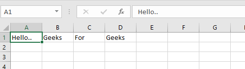
Code #1 : Using A1 notation(cell name) for writing data in the specific cells.
Python3
import xlsxwriter
workbook = xlsxwriter.Workbook('hello.xlsx')
worksheet = workbook.add_worksheet()
worksheet.write('A1', 'Hello..')
worksheet.write('B1', 'Geeks')
worksheet.write('C1', 'For')
worksheet.write('D1', 'Geeks')
workbook.close()
Output:
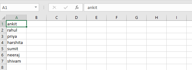
Code #2 : Using the row-column notation(indexing value) for writing data in the specific cells.
Python3
import xlsxwriter
workbook = xlsxwriter.Workbook('Example2.xlsx')
worksheet = workbook.add_worksheet()
row = 0
column = 0
content = ["ankit", "rahul", "priya", "harshita",
"sumit", "neeraj", "shivam"]
for item in content :
worksheet.write(row, column, item)
row += 1
workbook.close()
Output:
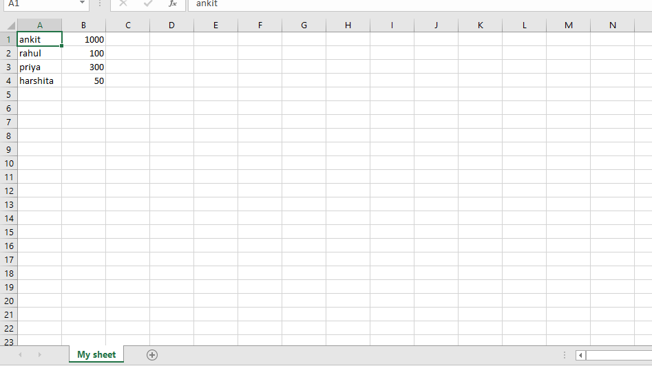
Code #3 : Creating a new sheet with the specific name
Python3
import xlsxwriter
workbook = xlsxwriter.Workbook('Example3.xlsx')
worksheet = workbook.add_worksheet("My sheet")
scores = (
['ankit', 1000],
['rahul', 100],
['priya', 300],
['harshita', 50],
)
row = 0
col = 0
for name, score in (scores):
worksheet.write(row, col, name)
worksheet.write(row, col + 1, score)
row += 1
workbook.close()
Output:
XlsxWriter has some advantages and disadvantages over the alternative Python modules for writing Excel files.
Advantages:
- It supports more Excel features than any of the alternative modules.
- It has a high degree of fidelity with files produced by Excel. In most cases the files produced are 100% equivalent to files produced by Excel.
- It has extensive documentation, example files and tests.
- It is fast and can be configured to use very little memory even for very large output files.
Disadvantages:
- It cannot read or modify existing Excel XLSX files.
Like Article
Save Article
Watch Now This tutorial has a related video course created by the Real Python team. Watch it together with the written tutorial to deepen your understanding: Editing Excel Spreadsheets in Python With openpyxl
Excel spreadsheets are one of those things you might have to deal with at some point. Either it’s because your boss loves them or because marketing needs them, you might have to learn how to work with spreadsheets, and that’s when knowing openpyxl comes in handy!
Spreadsheets are a very intuitive and user-friendly way to manipulate large datasets without any prior technical background. That’s why they’re still so commonly used today.
In this article, you’ll learn how to use openpyxl to:
- Manipulate Excel spreadsheets with confidence
- Extract information from spreadsheets
- Create simple or more complex spreadsheets, including adding styles, charts, and so on
This article is written for intermediate developers who have a pretty good knowledge of Python data structures, such as dicts and lists, but also feel comfortable around OOP and more intermediate level topics.
Before You Begin
If you ever get asked to extract some data from a database or log file into an Excel spreadsheet, or if you often have to convert an Excel spreadsheet into some more usable programmatic form, then this tutorial is perfect for you. Let’s jump into the openpyxl caravan!
Practical Use Cases
First things first, when would you need to use a package like openpyxl in a real-world scenario? You’ll see a few examples below, but really, there are hundreds of possible scenarios where this knowledge could come in handy.
Importing New Products Into a Database
You are responsible for tech in an online store company, and your boss doesn’t want to pay for a cool and expensive CMS system.
Every time they want to add new products to the online store, they come to you with an Excel spreadsheet with a few hundred rows and, for each of them, you have the product name, description, price, and so forth.
Now, to import the data, you’ll have to iterate over each spreadsheet row and add each product to the online store.
Exporting Database Data Into a Spreadsheet
Say you have a Database table where you record all your users’ information, including name, phone number, email address, and so forth.
Now, the Marketing team wants to contact all users to give them some discounted offer or promotion. However, they don’t have access to the Database, or they don’t know how to use SQL to extract that information easily.
What can you do to help? Well, you can make a quick script using openpyxl that iterates over every single User record and puts all the essential information into an Excel spreadsheet.
That’s gonna earn you an extra slice of cake at your company’s next birthday party!
Appending Information to an Existing Spreadsheet
You may also have to open a spreadsheet, read the information in it and, according to some business logic, append more data to it.
For example, using the online store scenario again, say you get an Excel spreadsheet with a list of users and you need to append to each row the total amount they’ve spent in your store.
This data is in the Database and, in order to do this, you have to read the spreadsheet, iterate through each row, fetch the total amount spent from the Database and then write back to the spreadsheet.
Not a problem for openpyxl!
Learning Some Basic Excel Terminology
Here’s a quick list of basic terms you’ll see when you’re working with Excel spreadsheets:
| Term | Explanation |
|---|---|
| Spreadsheet or Workbook | A Spreadsheet is the main file you are creating or working with. |
| Worksheet or Sheet | A Sheet is used to split different kinds of content within the same spreadsheet. A Spreadsheet can have one or more Sheets. |
| Column | A Column is a vertical line, and it’s represented by an uppercase letter: A. |
| Row | A Row is a horizontal line, and it’s represented by a number: 1. |
| Cell | A Cell is a combination of Column and Row, represented by both an uppercase letter and a number: A1. |
Getting Started With openpyxl
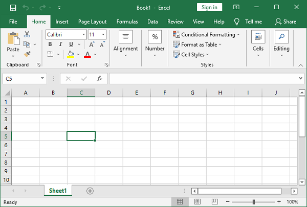
Now that you’re aware of the benefits of a tool like openpyxl, let’s get down to it and start by installing the package. For this tutorial, you should use Python 3.7 and openpyxl 2.6.2. To install the package, you can do the following:
After you install the package, you should be able to create a super simple spreadsheet with the following code:
from openpyxl import Workbook
workbook = Workbook()
sheet = workbook.active
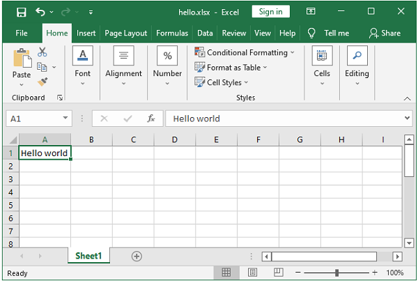
sheet["A1"] = "hello"
sheet["B1"] = "world!"
workbook.save(filename="hello_world.xlsx")
The code above should create a file called hello_world.xlsx in the folder you are using to run the code. If you open that file with Excel you should see something like this:
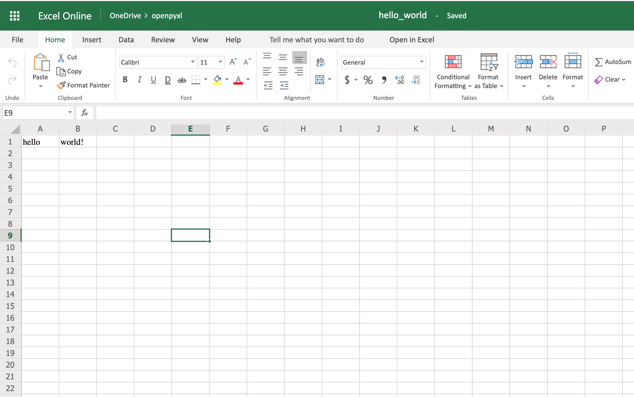
Woohoo, your first spreadsheet created!
Reading Excel Spreadsheets With openpyxl
Let’s start with the most essential thing one can do with a spreadsheet: read it.
You’ll go from a straightforward approach to reading a spreadsheet to more complex examples where you read the data and convert it into more useful Python structures.
Dataset for This Tutorial
Before you dive deep into some code examples, you should download this sample dataset and store it somewhere as sample.xlsx:
This is one of the datasets you’ll be using throughout this tutorial, and it’s a spreadsheet with a sample of real data from Amazon’s online product reviews. This dataset is only a tiny fraction of what Amazon provides, but for testing purposes, it’s more than enough.
A Simple Approach to Reading an Excel Spreadsheet
Finally, let’s start reading some spreadsheets! To begin with, open our sample spreadsheet:
>>>
>>> from openpyxl import load_workbook
>>> workbook = load_workbook(filename="sample.xlsx")
>>> workbook.sheetnames
['Sheet 1']

>>> sheet = workbook.active
>>> sheet
<Worksheet "Sheet 1">

>>> sheet.title
'Sheet 1'
In the code above, you first open the spreadsheet sample.xlsx using load_workbook(), and then you can use workbook.sheetnames to see all the sheets you have available to work with. After that, workbook.active selects the first available sheet and, in this case, you can see that it selects Sheet 1 automatically. Using these methods is the default way of opening a spreadsheet, and you’ll see it many times during this tutorial.
Now, after opening a spreadsheet, you can easily retrieve data from it like this:
>>>
>>> sheet["A1"]
<Cell 'Sheet 1'.A1>

>>> sheet["A1"].value
'marketplace'

>>> sheet["F10"].value
"G-Shock Men's Grey Sport Watch"
To return the actual value of a cell, you need to do .value. Otherwise, you’ll get the main Cell object. You can also use the method .cell() to retrieve a cell using index notation. Remember to add .value to get the actual value and not a Cell object:
>>>
>>> sheet.cell(row=10, column=6)
<Cell 'Sheet 1'.F10>

>>> sheet.cell(row=10, column=6).value
"G-Shock Men's Grey Sport Watch"
You can see that the results returned are the same, no matter which way you decide to go with. However, in this tutorial, you’ll be mostly using the first approach: ["A1"].
The above shows you the quickest way to open a spreadsheet. However, you can pass additional parameters to change the way a spreadsheet is loaded.
Additional Reading Options
There are a few arguments you can pass to load_workbook() that change the way a spreadsheet is loaded. The most important ones are the following two Booleans:
- read_only loads a spreadsheet in read-only mode allowing you to open very large Excel files.
- data_only ignores loading formulas and instead loads only the resulting values.
Importing Data From a Spreadsheet
Now that you’ve learned the basics about loading a spreadsheet, it’s about time you get to the fun part: the iteration and actual usage of the values within the spreadsheet.
This section is where you’ll learn all the different ways you can iterate through the data, but also how to convert that data into something usable and, more importantly, how to do it in a Pythonic way.
Iterating Through the Data
There are a few different ways you can iterate through the data depending on your needs.
You can slice the data with a combination of columns and rows:
>>>
>>> sheet["A1:C2"]
((<Cell 'Sheet 1'.A1>, <Cell 'Sheet 1'.B1>, <Cell 'Sheet 1'.C1>),
 (<Cell 'Sheet 1'.A2>, <Cell 'Sheet 1'.B2>, <Cell 'Sheet 1'.C2>))
You can get ranges of rows or columns:
>>>
>>> # Get all cells from column A
>>> sheet["A"]
(<Cell 'Sheet 1'.A1>,
 <Cell 'Sheet 1'.A2>,
 ...
 <Cell 'Sheet 1'.A99>,
 <Cell 'Sheet 1'.A100>)

>>> # Get all cells for a range of columns
>>> sheet["A:B"]
((<Cell 'Sheet 1'.A1>,
  <Cell 'Sheet 1'.A2>,
  ...
  <Cell 'Sheet 1'.A99>,
  <Cell 'Sheet 1'.A100>),
 (<Cell 'Sheet 1'.B1>,
  <Cell 'Sheet 1'.B2>,
  ...
  <Cell 'Sheet 1'.B99>,
  <Cell 'Sheet 1'.B100>))

>>> # Get all cells from row 5
>>> sheet[5]
(<Cell 'Sheet 1'.A5>,
 <Cell 'Sheet 1'.B5>,
 ...
 <Cell 'Sheet 1'.N5>,
 <Cell 'Sheet 1'.O5>)

>>> # Get all cells for a range of rows
>>> sheet[5:6]
((<Cell 'Sheet 1'.A5>,
  <Cell 'Sheet 1'.B5>,
  ...
  <Cell 'Sheet 1'.N5>,
  <Cell 'Sheet 1'.O5>),
 (<Cell 'Sheet 1'.A6>,
  <Cell 'Sheet 1'.B6>,
  ...
  <Cell 'Sheet 1'.N6>,
  <Cell 'Sheet 1'.O6>))
You’ll notice that all of the above examples return a tuple. If you want to refresh your memory on how to handle tuples in Python, check out the article on Lists and Tuples in Python.
There are also multiple ways of using normal Python generators to go through the data. The main methods you can use to achieve this are:
.iter_rows().iter_cols()
Both methods can receive the following arguments:
min_rowmax_rowmin_colmax_col
These arguments are used to set boundaries for the iteration:
>>>
>>> for row in sheet.iter_rows(min_row=1,
...                            max_row=2,
...                            min_col=1,
...                            max_col=3):
...     print(row)
(<Cell 'Sheet 1'.A1>, <Cell 'Sheet 1'.B1>, <Cell 'Sheet 1'.C1>)
(<Cell 'Sheet 1'.A2>, <Cell 'Sheet 1'.B2>, <Cell 'Sheet 1'.C2>)


>>> for column in sheet.iter_cols(min_row=1,
...                               max_row=2,
...                               min_col=1,
...                               max_col=3):
...     print(column)
(<Cell 'Sheet 1'.A1>, <Cell 'Sheet 1'.A2>)
(<Cell 'Sheet 1'.B1>, <Cell 'Sheet 1'.B2>)
(<Cell 'Sheet 1'.C1>, <Cell 'Sheet 1'.C2>)
You’ll notice that in the first example, when iterating through the rows using .iter_rows(), you get one tuple element per row selected. While when using .iter_cols() and iterating through columns, you’ll get one tuple per column instead.
One additional argument you can pass to both methods is the Boolean values_only. When it’s set to True, the values of the cell are returned, instead of the Cell object:
>>>
>>> for value in sheet.iter_rows(min_row=1,
...                              max_row=2,
...                              min_col=1,
...                              max_col=3,
...                              values_only=True):
...     print(value)
('marketplace', 'customer_id', 'review_id')
('US', 3653882, 'R3O9SGZBVQBV76')
If you want to iterate through the whole dataset, then you can also use the attributes .rows or .columns directly, which are shortcuts to using .iter_rows() and .iter_cols() without any arguments:
>>>
>>> for row in sheet.rows:
...     print(row)
(<Cell 'Sheet 1'.A1>, <Cell 'Sheet 1'.B1>, <Cell 'Sheet 1'.C1>
...
<Cell 'Sheet 1'.M100>, <Cell 'Sheet 1'.N100>, <Cell 'Sheet 1'.O100>)
These shortcuts are very useful when you’re iterating through the whole dataset.
Manipulate Data Using Python’s Default Data Structures
Now that you know the basics of iterating through the data in a workbook, let’s look at smart ways of converting that data into Python structures.
As you saw earlier, the result from all iterations comes in the form of tuples. However, since a tuple is nothing more than an immutable list, you can easily access its data and transform it into other structures.
For example, say you want to extract product information from the sample.xlsx spreadsheet and into a dictionary where each key is a product ID.
A straightforward way to do this is to iterate over all the rows, pick the columns you know are related to product information, and then store that in a dictionary. Let’s code this out!
First of all, have a look at the headers and see what information you care most about:
>>>
>>> for value in sheet.iter_rows(min_row=1,
...                              max_row=1,
...                              values_only=True):
...     print(value)
('marketplace', 'customer_id', 'review_id', 'product_id', ...)
This code returns a list of all the column names you have in the spreadsheet. To start, grab the columns with names:
product_idproduct_parentproduct_titleproduct_category
Lucky for you, the columns you need are all next to each other so you can use the min_column and max_column to easily get the data you want:
>>>
>>> for value in sheet.iter_rows(min_row=2,
...                              min_col=4,
...                              max_col=7,
...                              values_only=True):
...     print(value)
('B00FALQ1ZC', 937001370, 'Invicta Women's 15150 "Angel" 18k Yellow...)
('B00D3RGO20', 484010722, "Kenneth Cole New York Women's KC4944...)
...
Nice! Now that you know how to get all the important product information you need, let’s put that data into a dictionary:
import json
from openpyxl import load_workbook

workbook = load_workbook(filename="sample.xlsx")
sheet = workbook.active

products = {}

# Using the values_only because you want to return the cells' values
for row in sheet.iter_rows(min_row=2,
                           min_col=4,
                           max_col=7,
                           values_only=True):
    product_id = row[0]
    product = {
        "parent": row[1],
        "title": row[2],
        "category": row[3]
    }
    products[product_id] = product

# Using json here to be able to format the output for displaying later
print(json.dumps(products))
The code above returns a JSON similar to this:
{
  "B00FALQ1ZC": {
    "parent": 937001370,
    "title": "Invicta Women's 15150 ...",
    "category": "Watches"
  },
  "B00D3RGO20": {
    "parent": 484010722,
    "title": "Kenneth Cole New York ...",
    "category": "Watches"
  }
}
Here you can see that the output is trimmed to 2 products only, but if you run the script as it is, then you should get 98 products.
Convert Data Into Python Classes
To finalize the reading section of this tutorial, let’s dive into Python classes and see how you could improve on the example above and better structure the data.
For this, you’ll be using the new Python Data Classes that are available from Python 3.7. If you’re using an older version of Python, then you can use the default Classes instead.
So, first things first, let’s look at the data you have and decide what you want to store and how you want to store it.
As you saw right at the start, this data comes from Amazon, and it’s a list of product reviews. You can check the list of all the columns and their meaning on Amazon.
There are two significant elements you can extract from the data available:
- Products
- Reviews
A Product has:
- ID
- Title
- Parent
- Category
The Review has a few more fields:
- ID
- Customer ID
- Stars
- Headline
- Body
- Date
You can ignore a few of the review fields to make things a bit simpler.
So, a straightforward implementation of these two classes could be written in a separate file classes.py:
import datetime
from dataclasses import dataclass

@dataclass
class Product:
    id: str
    parent: str
    title: str
    category: str

@dataclass
class Review:
    id: str
    customer_id: str
    stars: int
    headline: str
    body: str
    date: datetime.datetime
After defining your data classes, you need to convert the data from the spreadsheet into these new structures.
Before doing the conversion, it’s worth looking at our header again and creating a mapping between columns and the fields you need:
>>>
>>> for value in sheet.iter_rows(min_row=1,
...                              max_row=1,
...                              values_only=True):
...     print(value)
('marketplace', 'customer_id', 'review_id', 'product_id', ...)

>>> # Or an alternative
>>> for cell in sheet[1]:
...     print(cell.value)
marketplace
customer_id
review_id
product_id
product_parent
...
Let’s create a file mapping.py where you have a list of all the field names and their column location (zero-indexed) on the spreadsheet:
# Product fields
PRODUCT_ID = 3
PRODUCT_PARENT = 4
PRODUCT_TITLE = 5
PRODUCT_CATEGORY = 6

# Review fields
REVIEW_ID = 2
REVIEW_CUSTOMER = 1
REVIEW_STARS = 7
REVIEW_HEADLINE = 12
REVIEW_BODY = 13
REVIEW_DATE = 14
You don’t necessarily have to do the mapping above. It’s more for readability when parsing the row data, so you don’t end up with a lot of magic numbers lying around.
Finally, let’s look at the code needed to parse the spreadsheet data into a list of product and review objects:
from datetime import datetime
from openpyxl import load_workbook
from classes import Product, Review
from mapping import PRODUCT_ID, PRODUCT_PARENT, PRODUCT_TITLE,
    PRODUCT_CATEGORY, REVIEW_DATE, REVIEW_ID, REVIEW_CUSTOMER,
    REVIEW_STARS, REVIEW_HEADLINE, REVIEW_BODY

# Using the read_only method since you're not gonna be editing the spreadsheet
workbook = load_workbook(filename="sample.xlsx", read_only=True)
sheet = workbook.active

products = []
reviews = []

# Using the values_only because you just want to return the cell value
for row in sheet.iter_rows(min_row=2, values_only=True):
    product = Product(id=row[PRODUCT_ID],
                      parent=row[PRODUCT_PARENT],
                      title=row[PRODUCT_TITLE],
                      category=row[PRODUCT_CATEGORY])
    products.append(product)

    # You need to parse the date from the spreadsheet into a datetime format
    spread_date = row[REVIEW_DATE]
    parsed_date = datetime.strptime(spread_date, "%Y-%m-%d")

    review = Review(id=row[REVIEW_ID],
                    customer_id=row[REVIEW_CUSTOMER],
                    stars=row[REVIEW_STARS],
                    headline=row[REVIEW_HEADLINE],
                    body=row[REVIEW_BODY],
                    date=parsed_date)
    reviews.append(review)

print(products[0])
print(reviews[0])
After you run the code above, you should get some output like this:
Product(id='B00FALQ1ZC', parent=937001370, ...)
Review(id='R3O9SGZBVQBV76', customer_id=3653882, ...)
That’s it! Now you should have the data in a very simple and digestible class format, and you can start thinking of storing this in a Database or any other type of data storage you like.
Using this kind of OOP strategy to parse spreadsheets makes handling the data much simpler later on.
Appending New Data
Before you start creating very complex spreadsheets, have a quick look at an example of how to append data to an existing spreadsheet.
Go back to the first example spreadsheet you created (hello_world.xlsx) and try opening it and appending some data to it, like this:
from openpyxl import load_workbook

# Start by opening the spreadsheet and selecting the main sheet
workbook = load_workbook(filename="hello_world.xlsx")
sheet = workbook.active

# Write what you want into a specific cell
sheet["C1"] = "writing ;)"

# Save the spreadsheet
workbook.save(filename="hello_world_append.xlsx")
Et voilà, if you open the new hello_world_append.xlsx spreadsheet, you’ll see the following change:
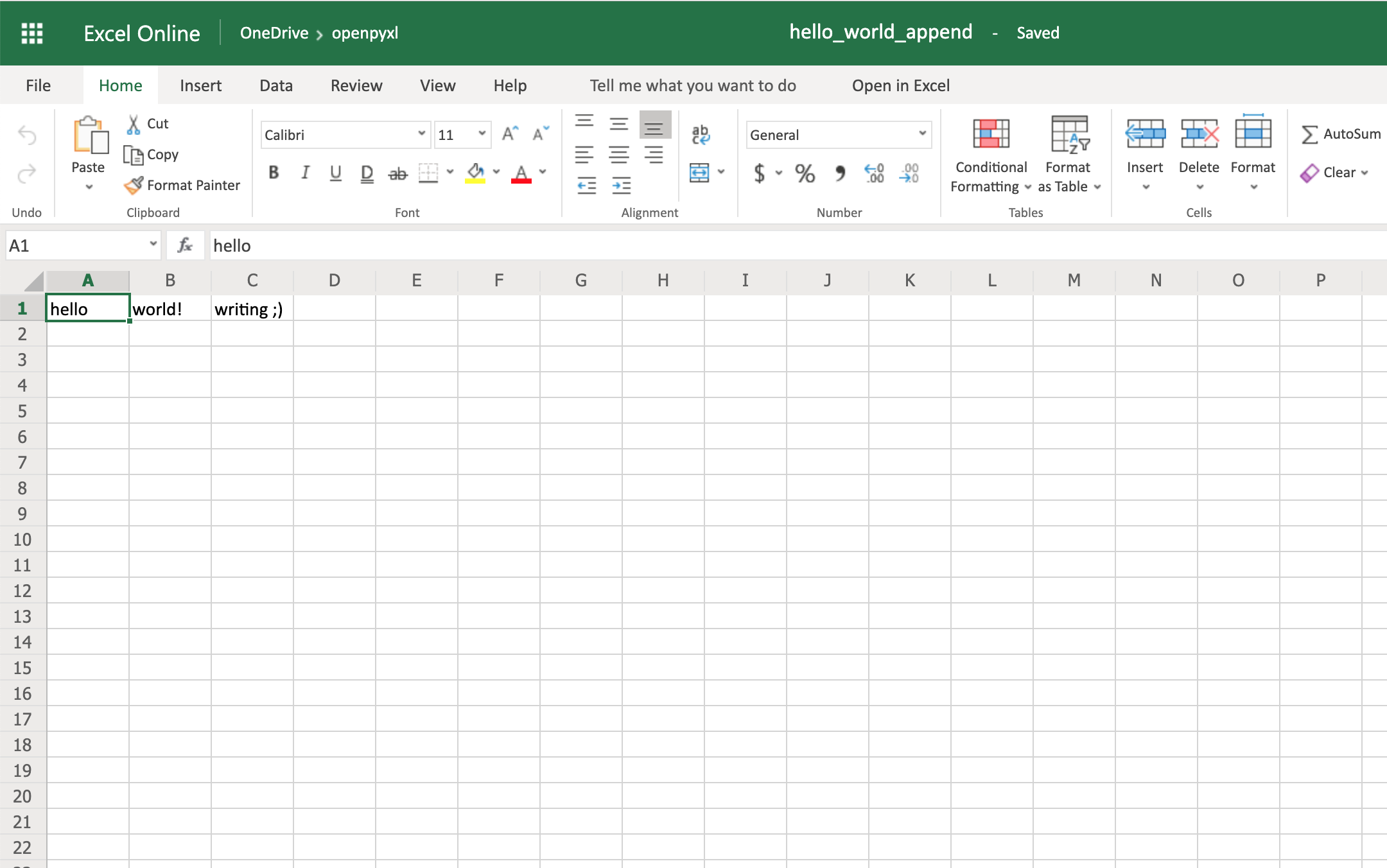
Notice the additional writing  on cell
 C1.
Writing Excel Spreadsheets With openpyxl
There are a lot of different things you can write to a spreadsheet, from simple text or number values to complex formulas, charts, or even images.
Let’s start creating some spreadsheets!
Creating a Simple Spreadsheet
Previously, you saw a very quick example of how to write “Hello world!” into a spreadsheet, so you can start with that:
 1from openpyxl import Workbook
 2
 3filename = "hello_world.xlsx"
 4
 5workbook = Workbook()
 6sheet = workbook.active
 7
 8sheet["A1"] = "hello"
 9sheet["B1"] = "world!"
10
11workbook.save(filename=filename)
The highlighted lines in the code above are the most important ones for writing. In the code, you can see that:
- Line 5 shows you how to create a new empty workbook.
- Lines 8 and 9 show you how to add data to specific cells.
- Line 11 shows you how to save the spreadsheet when you’re done.
Even though these lines above can be straightforward, it’s still good to know them well for when things get a bit more complicated.
One thing you can do to help with coming code examples is add the following method to your Python file or console:
>>>
>>> def print_rows():
...     for row in sheet.iter_rows(values_only=True):
...         print(row)
It makes it easier to print all of your spreadsheet values by just calling print_rows().
Basic Spreadsheet Operations
Before you get into the more advanced topics, it’s good for you to know how to manage the most simple elements of a spreadsheet.
Adding and Updating Cell Values
You already learned how to add values to a spreadsheet like this:
>>>
>>> sheet["A1"] = "value"
There’s another way you can do this, by first selecting a cell and then changing its value:
>>>
>>> cell = sheet["A1"]
>>> cell
<Cell 'Sheet'.A1>

>>> cell.value
'hello'

>>> cell.value = "hey"
>>> cell.value
'hey'
The new value is only stored into the spreadsheet once you call workbook.save().
The openpyxl creates a cell when adding a value, if that cell didn’t exist before:
>>>
>>> # Before, our spreadsheet has only 1 row
>>> print_rows()
('hello', 'world!')

>>> # Try adding a value to row 10
>>> sheet["B10"] = "test"
>>> print_rows()
('hello', 'world!')
(None, None)
(None, None)
(None, None)
(None, None)
(None, None)
(None, None)
(None, None)
(None, None)
(None, 'test')
As you can see, when trying to add a value to cell B10, you end up with a tuple with 10 rows, just so you can have that test value.
Managing Rows and Columns
One of the most common things you have to do when manipulating spreadsheets is adding or removing rows and columns. The openpyxl package allows you to do that in a very straightforward way by using the methods:
.insert_rows().delete_rows().insert_cols().delete_cols()
Every single one of those methods can receive two arguments:
idxamount
Using our basic hello_world.xlsx example again, let’s see how these methods work:
>>>
>>> print_rows()
('hello', 'world!')

>>> # Insert a column before the existing column 1 ("A")
>>> sheet.insert_cols(idx=1)
>>> print_rows()
(None, 'hello', 'world!')

>>> # Insert 5 columns between column 2 ("B") and 3 ("C")
>>> sheet.insert_cols(idx=3, amount=5)
>>> print_rows()
(None, 'hello', None, None, None, None, None, 'world!')

>>> # Delete the created columns
>>> sheet.delete_cols(idx=3, amount=5)
>>> sheet.delete_cols(idx=1)
>>> print_rows()
('hello', 'world!')

>>> # Insert a new row in the beginning
>>> sheet.insert_rows(idx=1)
>>> print_rows()
(None, None)
('hello', 'world!')

>>> # Insert 3 new rows in the beginning
>>> sheet.insert_rows(idx=1, amount=3)
>>> print_rows()
(None, None)
(None, None)
(None, None)
(None, None)
('hello', 'world!')

>>> # Delete the first 4 rows
>>> sheet.delete_rows(idx=1, amount=4)
>>> print_rows()
('hello', 'world!')
The only thing you need to remember is that when inserting new data (rows or columns), the insertion happens before the idx parameter.
So, if you do insert_rows(1), it inserts a new row before the existing first row.
It’s the same for columns: when you call insert_cols(2), it inserts a new column right before the already existing second column (B).
However, when deleting rows or columns, .delete_... deletes data starting from the index passed as an argument.
For example, when doing delete_rows(2) it deletes row 2, and when doing delete_cols(3) it deletes the third column (C).
Managing Sheets
Sheet management is also one of those things you might need to know, even though it might be something that you don’t use that often.
If you look back at the code examples from this tutorial, you’ll notice the following recurring piece of code:
This is the way to select the default sheet from a spreadsheet. However, if you’re opening a spreadsheet with multiple sheets, then you can always select a specific one like this:
>>>
>>> # Let's say you have two sheets: "Products" and "Company Sales"
>>> workbook.sheetnames
['Products', 'Company Sales']

>>> # You can select a sheet using its title
>>> products_sheet = workbook["Products"]
>>> sales_sheet = workbook["Company Sales"]
You can also change a sheet title very easily:
>>>
>>> workbook.sheetnames
['Products', 'Company Sales']

>>> products_sheet = workbook["Products"]
>>> products_sheet.title = "New Products"

>>> workbook.sheetnames
['New Products', 'Company Sales']
If you want to create or delete sheets, then you can also do that with .create_sheet() and .remove():
>>>
>>> workbook.sheetnames
['Products', 'Company Sales']

>>> operations_sheet = workbook.create_sheet("Operations")
>>> workbook.sheetnames
['Products', 'Company Sales', 'Operations']

>>> # You can also define the position to create the sheet at
>>> hr_sheet = workbook.create_sheet("HR", 0)
>>> workbook.sheetnames
['HR', 'Products', 'Company Sales', 'Operations']

>>> # To remove them, just pass the sheet as an argument to the .remove()
>>> workbook.remove(operations_sheet)
>>> workbook.sheetnames
['HR', 'Products', 'Company Sales']

>>> workbook.remove(hr_sheet)
>>> workbook.sheetnames
['Products', 'Company Sales']
One other thing you can do is make duplicates of a sheet using copy_worksheet():
>>>
>>> workbook.sheetnames
['Products', 'Company Sales']

>>> products_sheet = workbook["Products"]
>>> workbook.copy_worksheet(products_sheet)
<Worksheet "Products Copy">

>>> workbook.sheetnames
['Products', 'Company Sales', 'Products Copy']
If you open your spreadsheet after saving the above code, you’ll notice that the sheet Products Copy is a duplicate of the sheet Products.
Freezing Rows and Columns
Something that you might want to do when working with big spreadsheets is to freeze a few rows or columns, so they remain visible when you scroll right or down.
Freezing data allows you to keep an eye on important rows or columns, regardless of where you scroll in the spreadsheet.
Again, openpyxl also has a way to accomplish this by using the worksheet freeze_panes attribute. For this example, go back to our sample.xlsx spreadsheet and try doing the following:
>>>
>>> workbook = load_workbook(filename="sample.xlsx")
>>> sheet = workbook.active
>>> sheet.freeze_panes = "C2"
>>> workbook.save("sample_frozen.xlsx")
If you open the sample_frozen.xlsx spreadsheet in your favorite spreadsheet editor, you’ll notice that row 1 and columns A and B are frozen and are always visible no matter where you navigate within the spreadsheet.
This feature is handy, for example, to keep headers within sight, so you always know what each column represents.
Here’s how it looks in the editor:
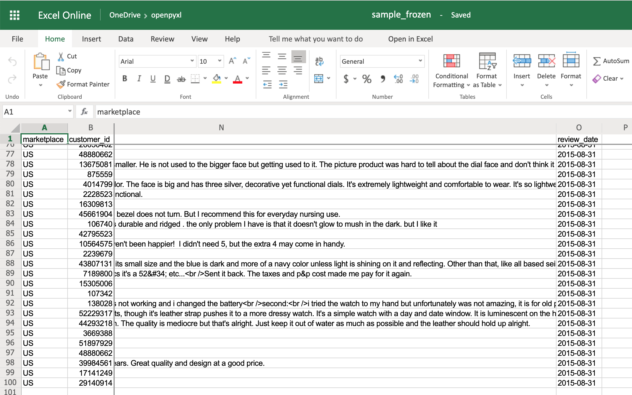
Notice how you’re at the end of the spreadsheet, and yet, you can see both row 1 and columns A and B.
Adding Filters
You can use openpyxl to add filters and sorts to your spreadsheet. However, when you open the spreadsheet, the data won’t be rearranged according to these sorts and filters.
At first, this might seem like a pretty useless feature, but when you’re programmatically creating a spreadsheet that is going to be sent and used by somebody else, it’s still nice to at least create the filters and allow people to use it afterward.
The code below is an example of how you would add some filters to our existing sample.xlsx spreadsheet:
>>>
>>> # Check the used spreadsheet space using the attribute "dimensions"
>>> sheet.dimensions
'A1:O100'

>>> sheet.auto_filter.ref = "A1:O100"
>>> workbook.save(filename="sample_with_filters.xlsx")
You should now see the filters created when opening the spreadsheet in your editor:
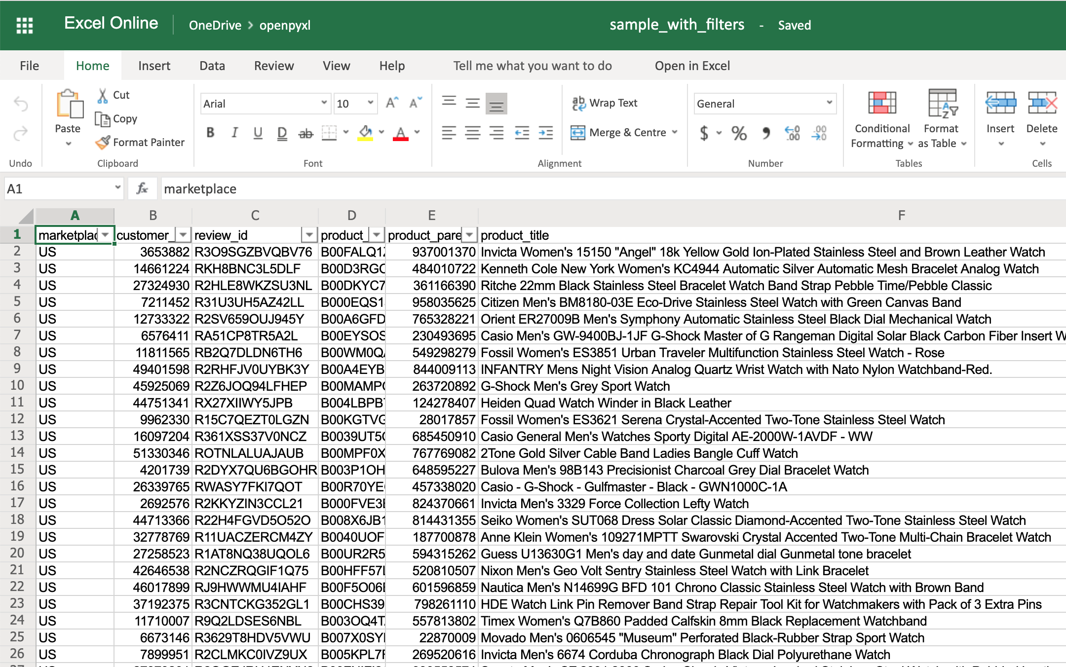
You don’t have to use sheet.dimensions if you know precisely which part of the spreadsheet you want to apply filters to.
Adding Formulas
Formulas (or formulae) are one of the most powerful features of spreadsheets.
They gives you the power to apply specific mathematical equations to a range of cells. Using formulas with openpyxl is as simple as editing the value of a cell.
You can see the list of formulas supported by openpyxl:
>>>
>>> from openpyxl.utils import FORMULAE
>>> FORMULAE
frozenset({'ABS',
           'ACCRINT',
           'ACCRINTM',
           'ACOS',
           'ACOSH',
           'AMORDEGRC',
           'AMORLINC',
           'AND',
           ...
           'YEARFRAC',
           'YIELD',
           'YIELDDISC',
           'YIELDMAT',
           'ZTEST'})
Let’s add some formulas to our sample.xlsx spreadsheet.
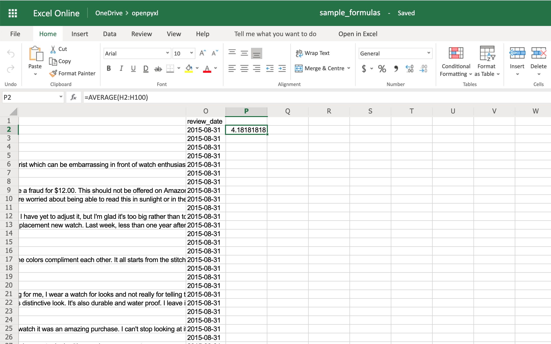
Starting with something easy, let’s check the average star rating for the 99 reviews within the spreadsheet:
>>>
>>> # Star rating is column "H"
>>> sheet["P2"] = "=AVERAGE(H2:H100)"
>>> workbook.save(filename="sample_formulas.xlsx")
If you open the spreadsheet now and go to cell P2, you should see that its value is: 4.18181818181818. Have a look in the editor:
You can use the same methodology to add any formulas to your spreadsheet. For example, let’s count the number of reviews that had helpful votes:
>>>
>>> # The helpful votes are counted on column "I"
>>> sheet["P3"] = '=COUNTIF(I2:I100, ">0")'
>>> workbook.save(filename="sample_formulas.xlsx")
You should get the number 21 on your P3 spreadsheet cell like so:
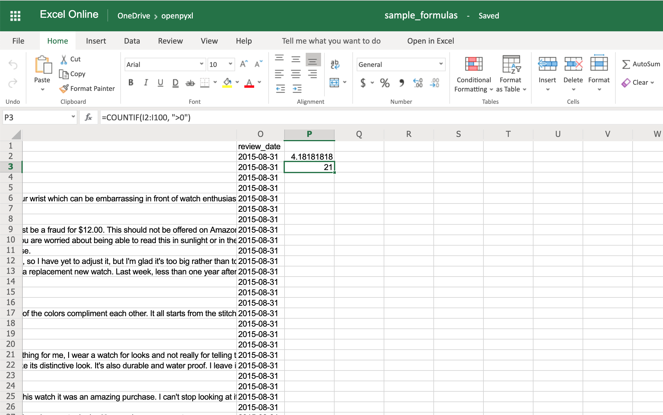
You’ll have to make sure that the strings within a formula are always in double quotes, so you either have to use single quotes around the formula like in the example above or you’ll have to escape the double quotes inside the formula: "=COUNTIF(I2:I100, ">0")".
There are a ton of other formulas you can add to your spreadsheet using the same procedure you tried above. Give it a go yourself!
Adding Styles
Even though styling a spreadsheet might not be something you would do every day, it’s still good to know how to do it.
Using openpyxl, you can apply multiple styling options to your spreadsheet, including fonts, borders, colors, and so on. Have a look at the openpyxl documentation to learn more.
You can also choose to either apply a style directly to a cell or create a template and reuse it to apply styles to multiple cells.
Let’s start by having a look at simple cell styling, using our sample.xlsx again as the base spreadsheet:
>>>
>>> # Import necessary style classes
>>> from openpyxl.styles import Font, Color, Alignment, Border, Side

>>> # Create a few styles
>>> bold_font = Font(bold=True)
>>> big_red_text = Font(color="00FF0000", size=20)
>>> center_aligned_text = Alignment(horizontal="center")
>>> double_border_side = Side(border_style="double")
>>> square_border = Border(top=double_border_side,
...                        right=double_border_side,
...                        bottom=double_border_side,
...                        left=double_border_side)

>>> # Style some cells!
>>> sheet["A2"].font = bold_font
>>> sheet["A3"].font = big_red_text
>>> sheet["A4"].alignment = center_aligned_text
>>> sheet["A5"].border = square_border
>>> workbook.save(filename="sample_styles.xlsx")
If you open your spreadsheet now, you should see quite a few different styles on the first 5 cells of column A:
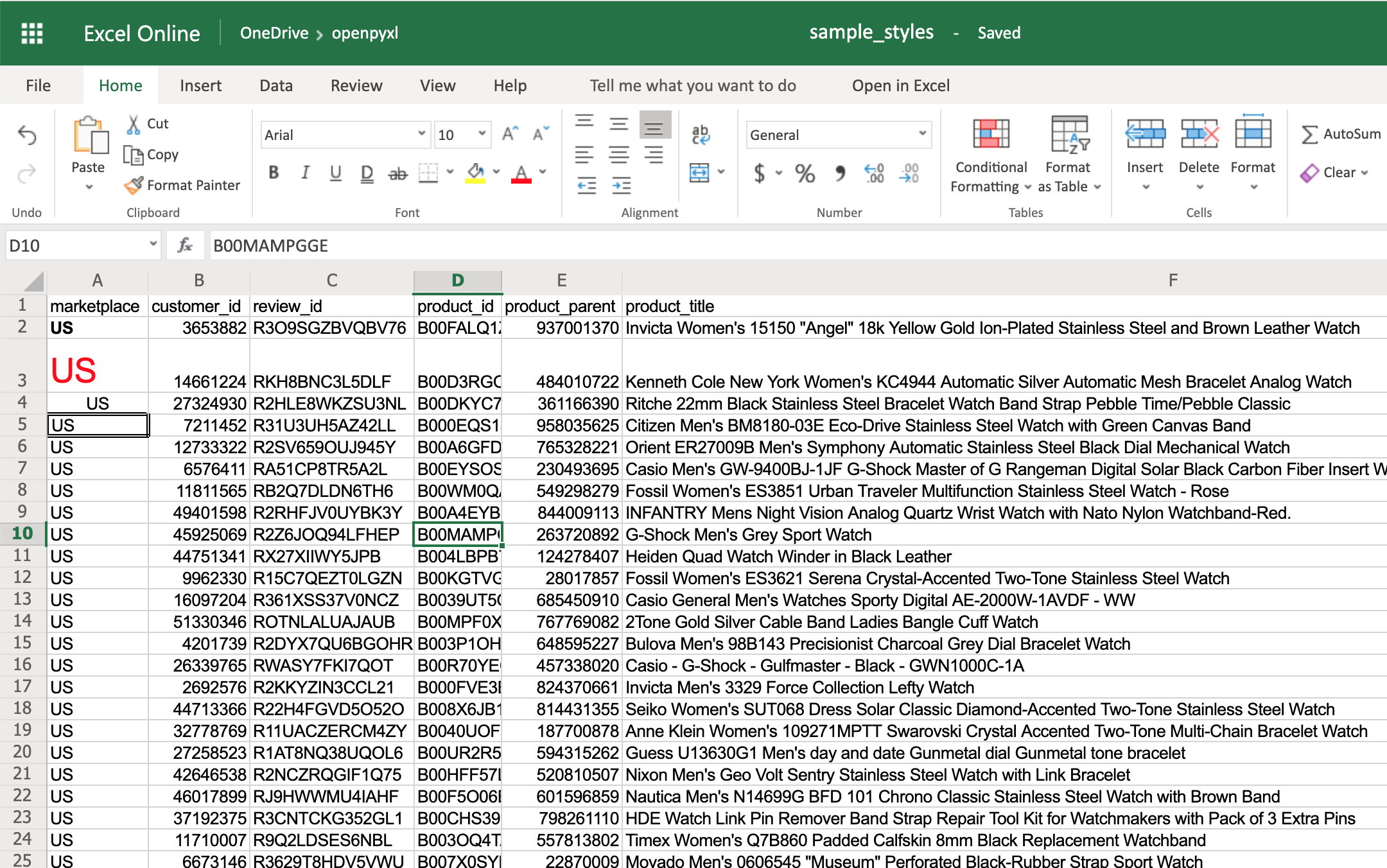
There you go. You got:
- A2 with the text in bold
- A3 with the text in red and bigger font size
- A4 with the text centered
- A5 with a square border around the text
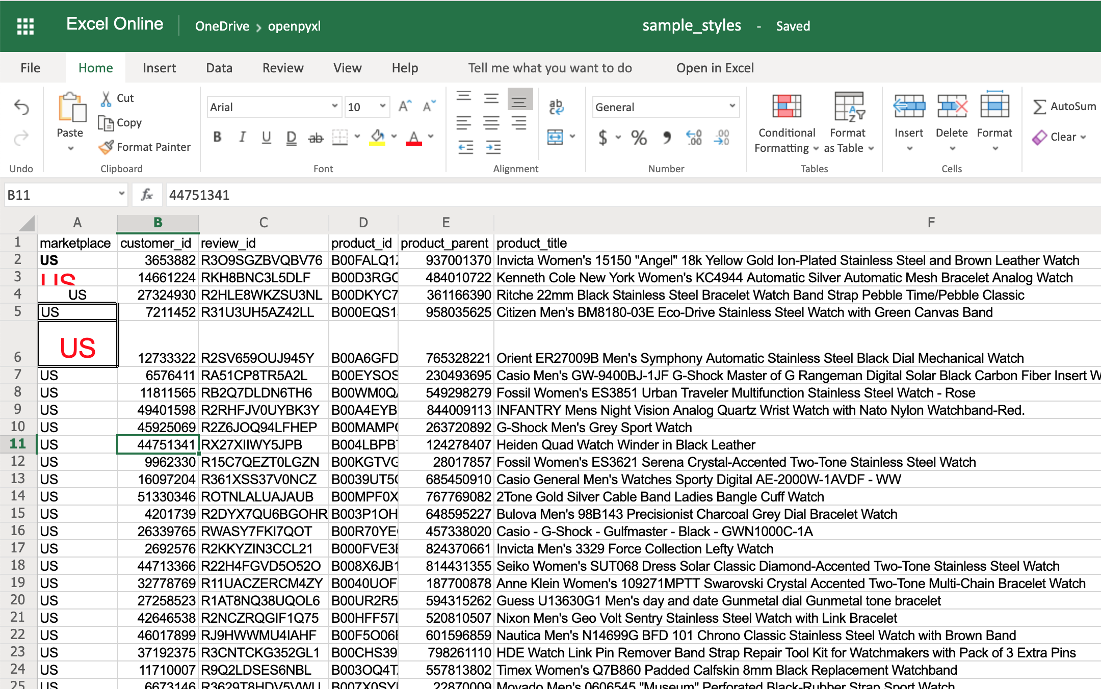
You can also combine styles by simply adding them to the cell at the same time:
>>>
>>> # Reusing the same styles from the example above
>>> sheet["A6"].alignment = center_aligned_text
>>> sheet["A6"].font = big_red_text
>>> sheet["A6"].border = square_border
>>> workbook.save(filename="sample_styles.xlsx")
Have a look at cell A6 here:
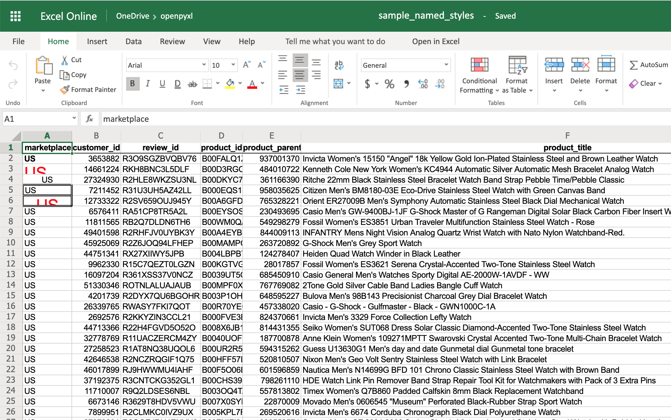
When you want to apply multiple styles to one or several cells, you can use a NamedStyle class instead, which is like a style template that you can use over and over again. Have a look at the example below:
>>>
>>> from openpyxl.styles import NamedStyle

>>> # Let's create a style template for the header row
>>> header = NamedStyle(name="header")
>>> header.font = Font(bold=True)
>>> header.border = Border(bottom=Side(border_style="thin"))
>>> header.alignment = Alignment(horizontal="center", vertical="center")

>>> # Now let's apply this to all first row (header) cells
>>> header_row = sheet[1]
>>> for cell in header_row:
...     cell.style = header

>>> workbook.save(filename="sample_styles.xlsx")
If you open the spreadsheet now, you should see that its first row is bold, the text is aligned to the center, and there’s a small bottom border! Have a look below:
As you saw above, there are many options when it comes to styling, and it depends on the use case, so feel free to check openpyxl documentation and see what other things you can do.
Conditional Formatting
This feature is one of my personal favorites when it comes to adding styles to a spreadsheet.
It’s a much more powerful approach to styling because it dynamically applies styles according to how the data in the spreadsheet changes.
In a nutshell, conditional formatting allows you to specify a list of styles to apply to a cell (or cell range) according to specific conditions.
For example, a widespread use case is to have a balance sheet where all the negative totals are in red, and the positive ones are in green. This formatting makes it much more efficient to spot good vs bad periods.
Without further ado, let’s pick our favorite spreadsheet—sample.xlsx—and add some conditional formatting.
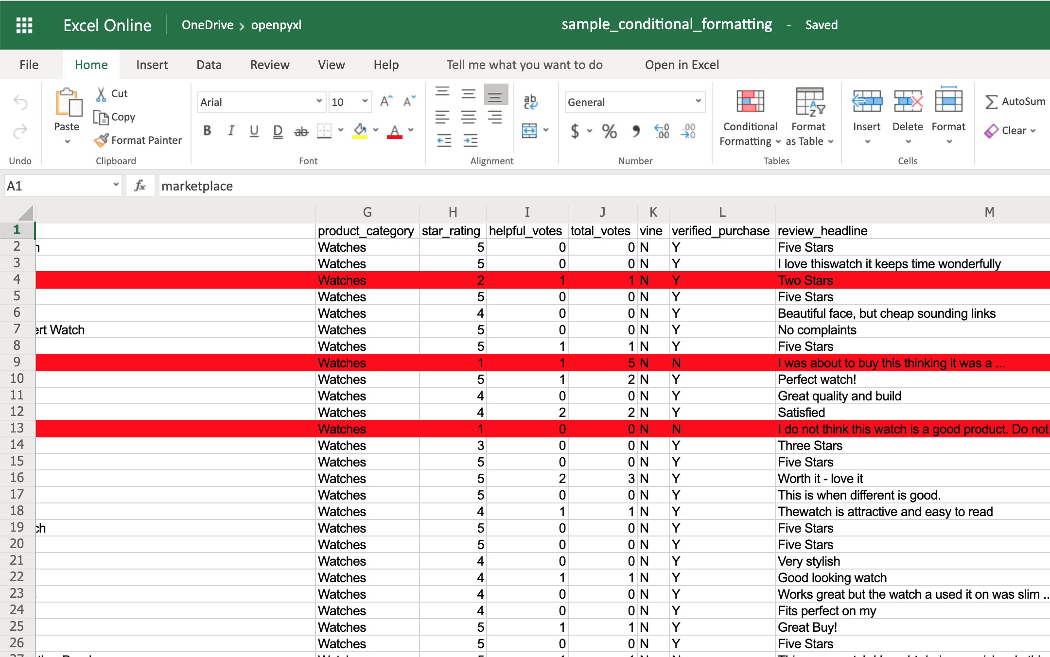
You can start by adding a simple one that adds a red background to all reviews with less than 3 stars:
>>>
>>> from openpyxl.styles import PatternFill
>>> from openpyxl.styles.differential import DifferentialStyle
>>> from openpyxl.formatting.rule import Rule

>>> red_background = PatternFill(fgColor="00FF0000")
>>> diff_style = DifferentialStyle(fill=red_background)
>>> rule = Rule(type="expression", dxf=diff_style)
>>> rule.formula = ["$H1<3"]
>>> sheet.conditional_formatting.add("A1:O100", rule)
>>> workbook.save("sample_conditional_formatting.xlsx")
Now you’ll see all the reviews with a star rating below 3 marked with a red background:
Code-wise, the only things that are new here are the objects DifferentialStyle and Rule:
DifferentialStyleis quite similar toNamedStyle, which you already saw above, and it’s used to aggregate multiple styles such as fonts, borders, alignment, and so forth.Ruleis responsible for selecting the cells and applying the styles if the cells match the rule’s logic.
Using a Rule object, you can create numerous conditional formatting scenarios.
However, for simplicity sake, the openpyxl package offers 3 built-in formats that make it easier to create a few common conditional formatting patterns. These built-ins are:
ColorScaleIconSetDataBar
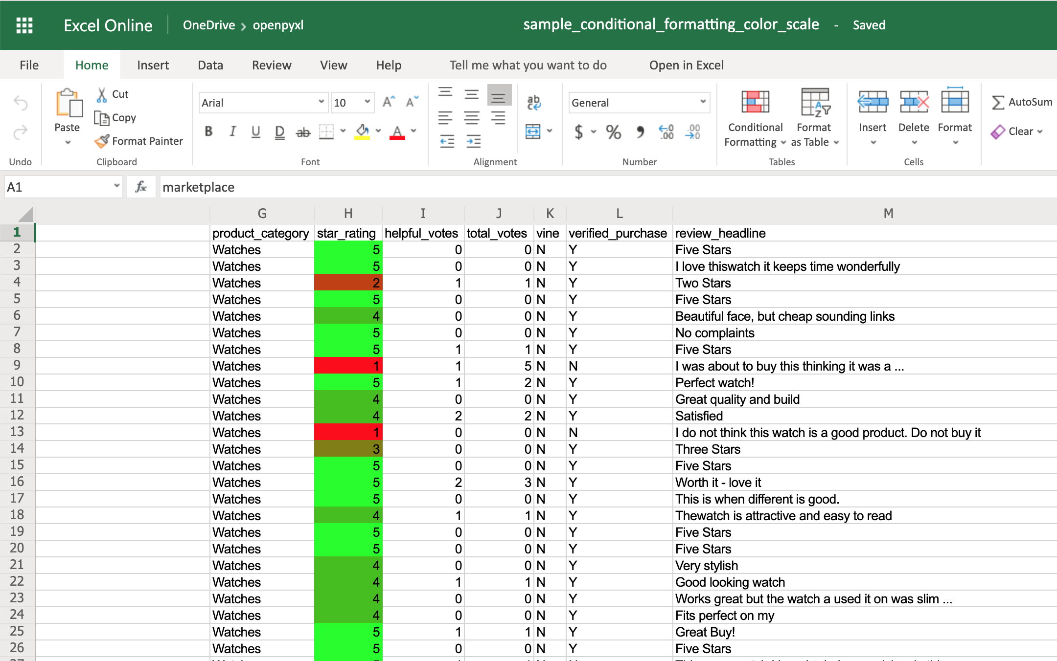
The ColorScale gives you the ability to create color gradients:
>>>
>>> from openpyxl.formatting.rule import ColorScaleRule
>>> color_scale_rule = ColorScaleRule(start_type="min",
...                                   start_color="00FF0000",  # Red
...                                   end_type="max",
...                                   end_color="0000FF00")  # Green

>>> # Again, let's add this gradient to the star ratings, column "H"
>>> sheet.conditional_formatting.add("H2:H100", color_scale_rule)
>>> workbook.save(filename="sample_conditional_formatting_color_scale.xlsx")
Now you should see a color gradient on column H, from red to green, according to the star rating:
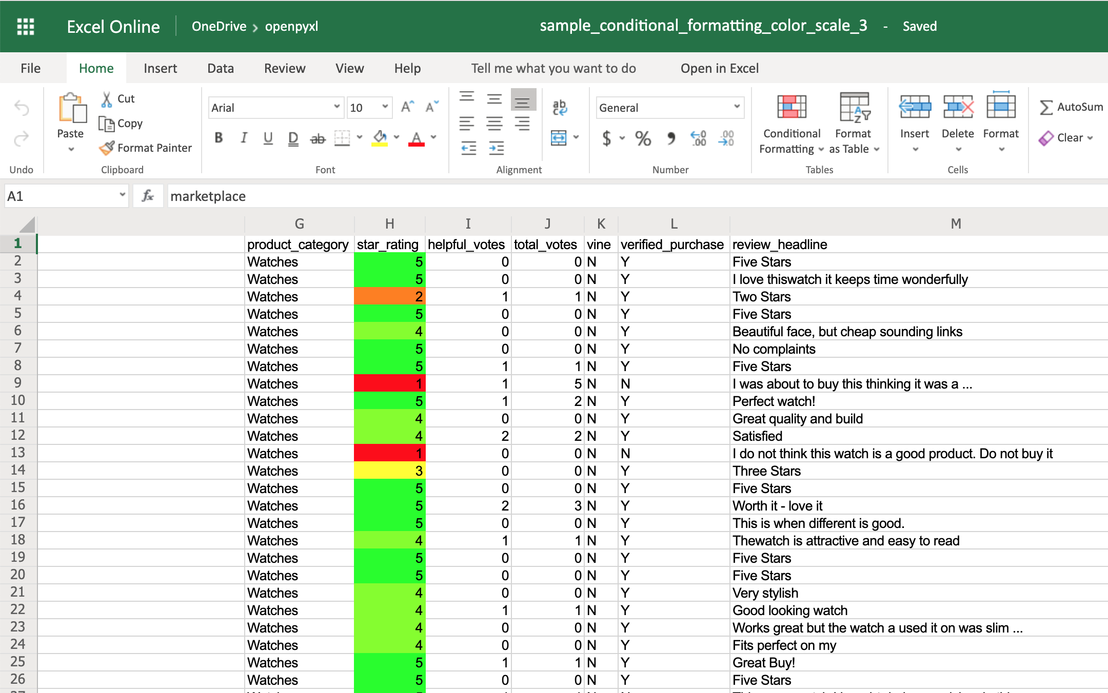
You can also add a third color and make two gradients instead:
>>>
>>> from openpyxl.formatting.rule import ColorScaleRule
>>> color_scale_rule = ColorScaleRule(start_type="num",
...                                   start_value=1,
...                                   start_color="00FF0000",  # Red
...                                   mid_type="num",
...                                   mid_value=3,
...                                   mid_color="00FFFF00",  # Yellow
...                                   end_type="num",
...                                   end_value=5,
...                                   end_color="0000FF00")  # Green

>>> # Again, let's add this gradient to the star ratings, column "H"
>>> sheet.conditional_formatting.add("H2:H100", color_scale_rule)
>>> workbook.save(filename="sample_conditional_formatting_color_scale_3.xlsx")
This time, you’ll notice that star ratings between 1 and 3 have a gradient from red to yellow, and star ratings between 3 and 5 have a gradient from yellow to green:
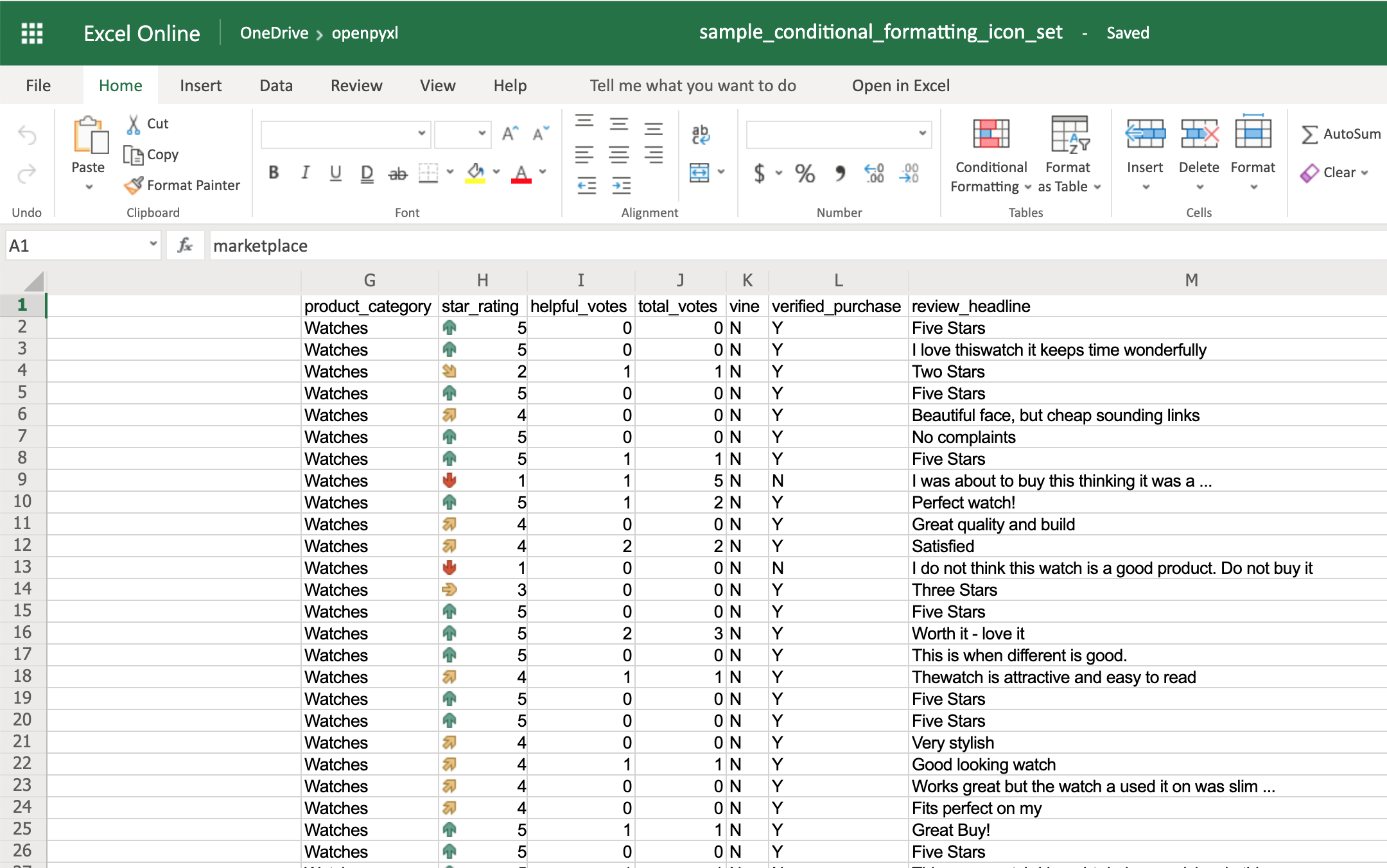
The IconSet allows you to add an icon to the cell according to its value:
>>>
>>> from openpyxl.formatting.rule import IconSetRule

>>> icon_set_rule = IconSetRule("5Arrows", "num", [1, 2, 3, 4, 5])
>>> sheet.conditional_formatting.add("H2:H100", icon_set_rule)
>>> workbook.save("sample_conditional_formatting_icon_set.xlsx")
You’ll see a colored arrow next to the star rating. This arrow is red and points down when the value of the cell is 1 and, as the rating gets better, the arrow starts pointing up and becomes green:
The openpyxl package has a full list of other icons you can use, besides the arrow.
Finally, the DataBar allows you to create progress bars:
>>>
>>> from openpyxl.formatting.rule import DataBarRule
>>> data_bar_rule = DataBarRule(start_type="num",
... start_value=1,
... end_type="num",
... end_value="5",
... color="0000FF00") # Green
>>> sheet.conditional_formatting.add("H2:H100", data_bar_rule)
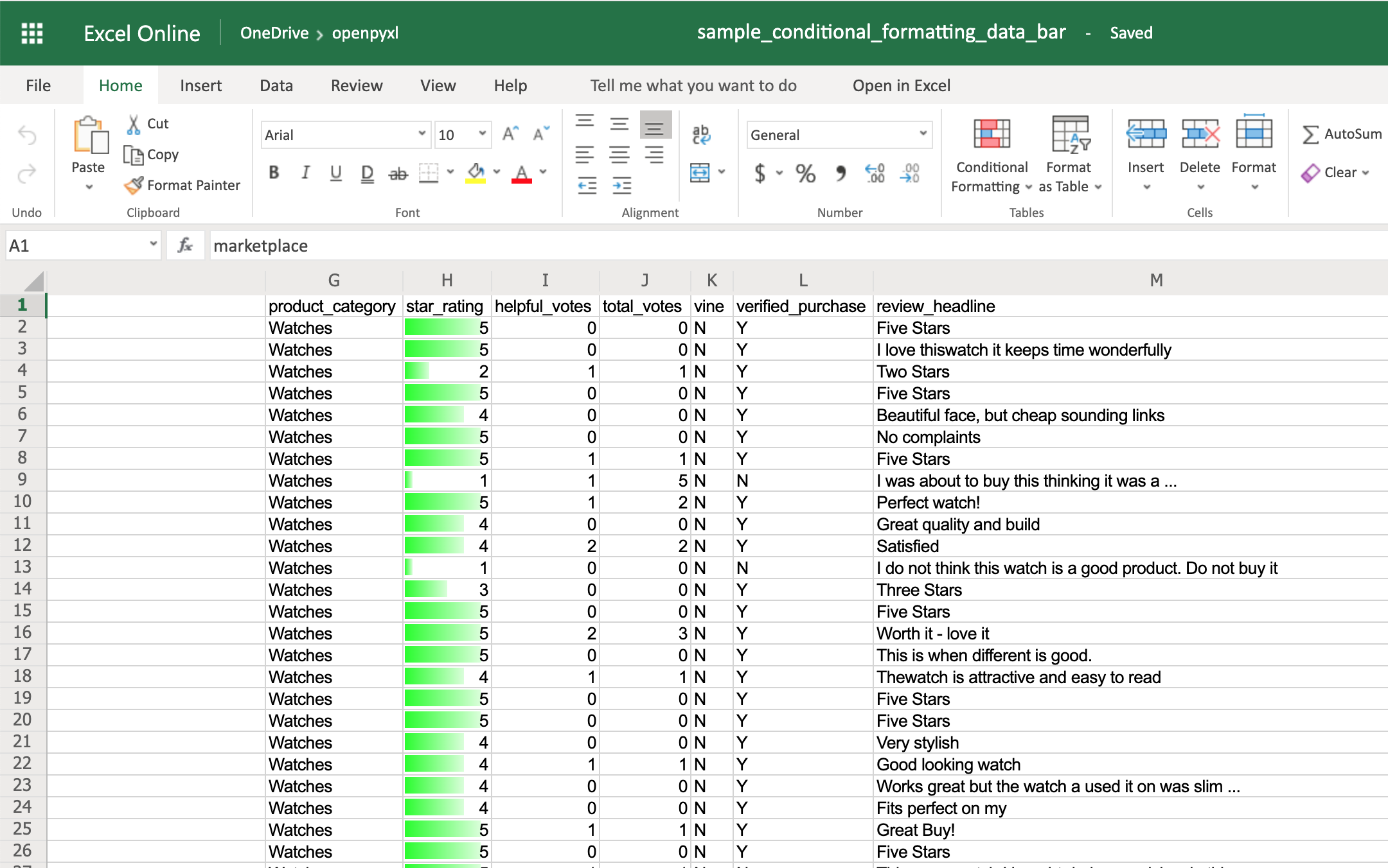
>>> workbook.save("sample_conditional_formatting_data_bar.xlsx")
You’ll now see a green progress bar that gets fuller the closer the star rating is to the number 5:
As you can see, there are a lot of cool things you can do with conditional formatting.
Here, you saw only a few examples of what you can achieve with it, but check the openpyxl documentation to see a bunch of other options.
Adding Images
Even though images are not something that you’ll often see in a spreadsheet, it’s quite cool to be able to add them. Maybe you can use it for branding purposes or to make spreadsheets more personal.
To be able to load images to a spreadsheet using openpyxl, you’ll have to install Pillow:
Apart from that, you’ll also need an image. For this example, you can grab the Real Python logo below and convert it from .webp to .png using an online converter such as cloudconvert.com, save the final file as logo.png, and copy it to the root folder where you’re running your examples:
![]()
Afterward, this is the code you need to import that image into the hello_word.xlsx spreadsheet:
from openpyxl import load_workbook
from openpyxl.drawing.image import Image

# Let's use the hello_world spreadsheet since it has less data
workbook = load_workbook(filename="hello_world.xlsx")
sheet = workbook.active

logo = Image("logo.png")

# A bit of resizing to not fill the whole spreadsheet with the logo
logo.height = 150
logo.width = 150

sheet.add_image(logo, "A3")
workbook.save(filename="hello_world_logo.xlsx")
You have an image on your spreadsheet! Here it is:
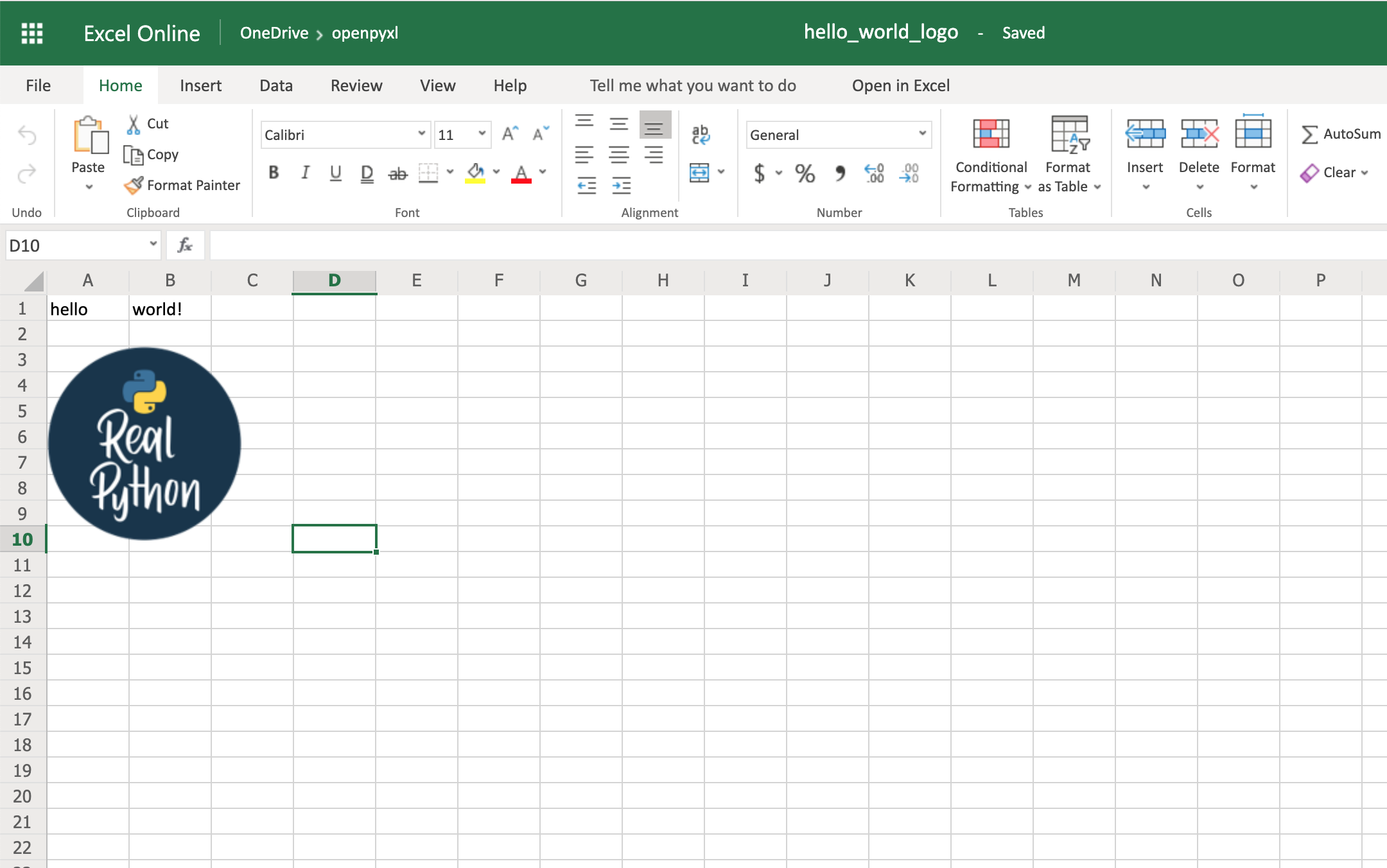
The image’s left top corner is on the cell you chose, in this case, A3.
Adding Pretty Charts
Another powerful thing you can do with spreadsheets is create an incredible variety of charts.
Charts are a great way to visualize and understand loads of data quickly. There are a lot of different chart types: bar chart, pie chart, line chart, and so on. openpyxl has support for a lot of them.
Here, you’ll see only a couple of examples of charts because the theory behind it is the same for every single chart type:
For any chart you want to build, you’ll need to define the chart type: BarChart, LineChart, and so forth, plus the data to be used for the chart, which is called Reference.
Before you can build your chart, you need to define what data you want to see represented in it. Sometimes, you can use the dataset as is, but other times you need to massage the data a bit to get additional information.
Let’s start by building a new workbook with some sample data:
 1from openpyxl import Workbook
 2from openpyxl.chart import BarChart, Reference
 3
 4workbook = Workbook()
 5sheet = workbook.active
 6
 7# Let's create some sample sales data
 8rows = [
 9    ["Product", "Online", "Store"],
10    [1, 30, 45],
11    [2, 40, 30],
12    [3, 40, 25],
13    [4, 50, 30],
14    [5, 30, 25],
15    [6, 25, 35],
16    [7, 20, 40],
17]
18
19for row in rows:
20    sheet.append(row)
Now you’re going to start by creating a bar chart that displays the total number of sales per product:
22chart = BarChart()
23data = Reference(worksheet=sheet,
24                 min_row=1,
25                 max_row=8,
26                 min_col=2,
27                 max_col=3)
28
29chart.add_data(data, titles_from_data=True)
30sheet.add_chart(chart, "E2")
31
32workbook.save("chart.xlsx")
There you have it. Below, you can see a very straightforward bar chart showing the difference between online product sales online and in-store product sales:
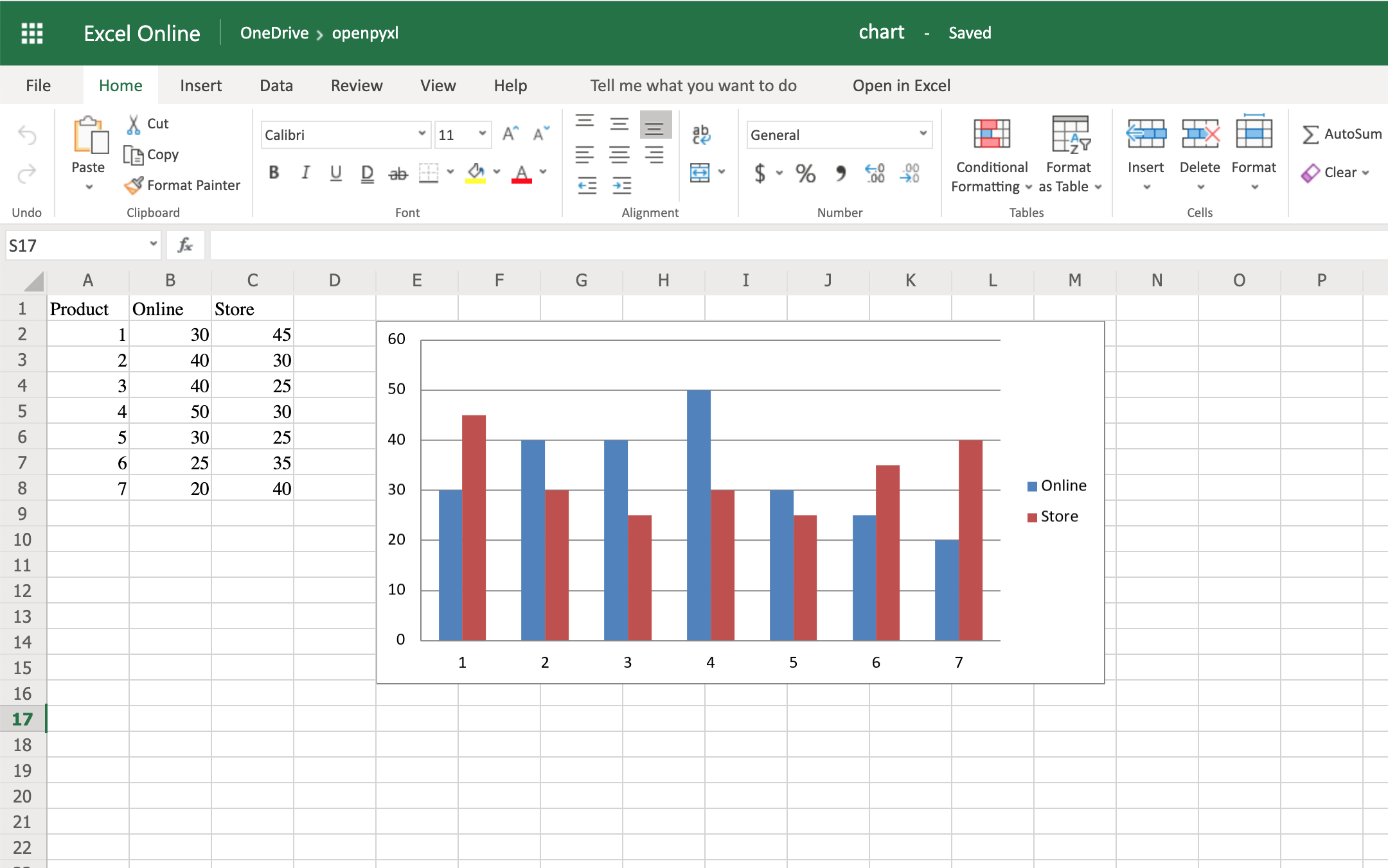
Like with images, the top left corner of the chart is on the cell you added the chart to. In your case, it was on cell E2.
Try creating a line chart instead, changing the data a bit:
 1import random
 2from openpyxl import Workbook
 3from openpyxl.chart import LineChart, Reference
 4
 5workbook = Workbook()
 6sheet = workbook.active
 7
 8# Let's create some sample sales data
 9rows = [
10    ["", "January", "February", "March", "April",
11    "May", "June", "July", "August", "September",
12     "October", "November", "December"],
13    [1, ],
14    [2, ],
15    [3, ],
16]
17
18for row in rows:
19    sheet.append(row)
20
21for row in sheet.iter_rows(min_row=2,
22                           max_row=4,
23                           min_col=2,
24                           max_col=13):
25    for cell in row:
26        cell.value = random.randrange(5, 100)
With the above code, you’ll be able to generate some random data regarding the sales of 3 different products across a whole year.
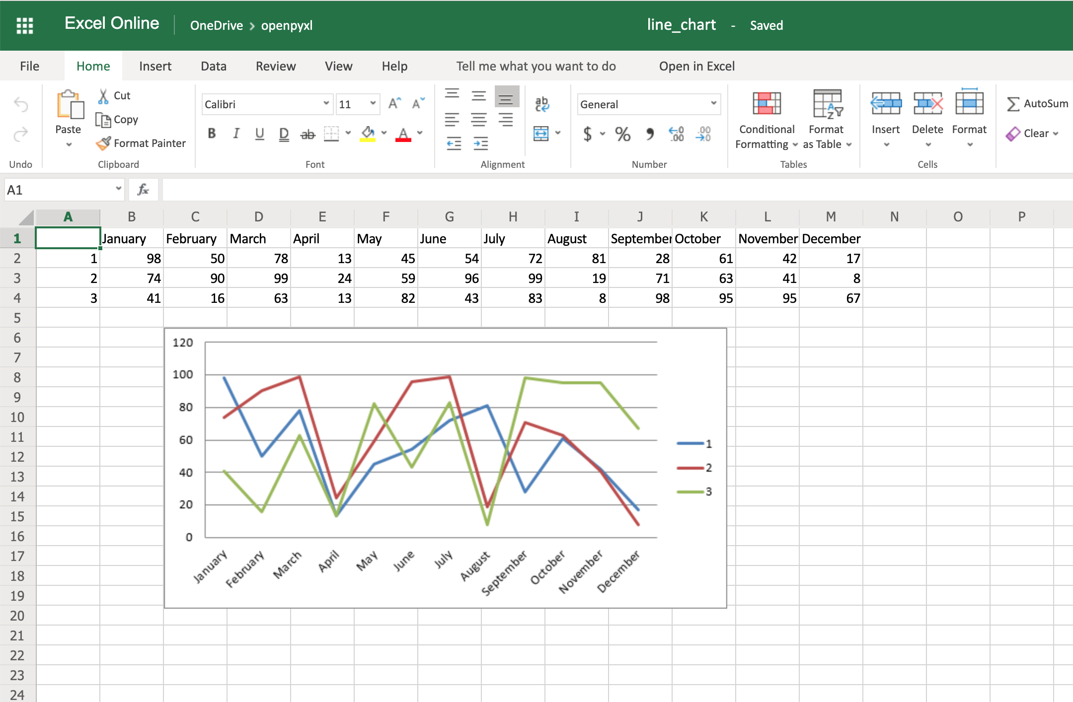
Once that’s done, you can very easily create a line chart with the following code:
28chart = LineChart()
29data = Reference(worksheet=sheet,
30                 min_row=2,
31                 max_row=4,
32                 min_col=1,
33                 max_col=13)
34
35chart.add_data(data, from_rows=True, titles_from_data=True)
36sheet.add_chart(chart, "C6")
37
38workbook.save("line_chart.xlsx")
Here’s the outcome of the above piece of code:
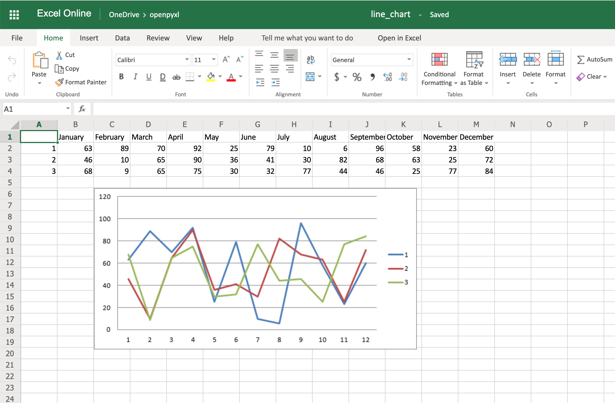
One thing to keep in mind here is the fact that you’re using from_rows=True when adding the data. This argument makes the chart plot row by row instead of column by column.
In your sample data, you see that each product has a row with 12 values (1 column per month). That’s why you use from_rows. If you don’t pass that argument, by default, the chart tries to plot by column, and you’ll get a month-by-month comparison of sales.
Another difference that has to do with the above argument change is the fact that our Reference now starts from the first column, min_col=1, instead of the second one. This change is needed because the chart now expects the first column to have the titles.
There are a couple of other things you can also change regarding the style of the chart. For example, you can add specific categories to the chart:
cats = Reference(worksheet=sheet,
                 min_row=1,
                 max_row=1,
                 min_col=2,
                 max_col=13)
chart.set_categories(cats)
Add this piece of code before saving the workbook, and you should see the month names appearing instead of numbers:
Code-wise, this is a minimal change. But in terms of the readability of the spreadsheet, this makes it much easier for someone to open the spreadsheet and understand the chart straight away.
Another thing you can do to improve the chart readability is to add an axis. You can do it using the attributes x_axis and y_axis:
chart.x_axis.title = "Months"
chart.y_axis.title = "Sales (per unit)"
This will generate a spreadsheet like the below one:
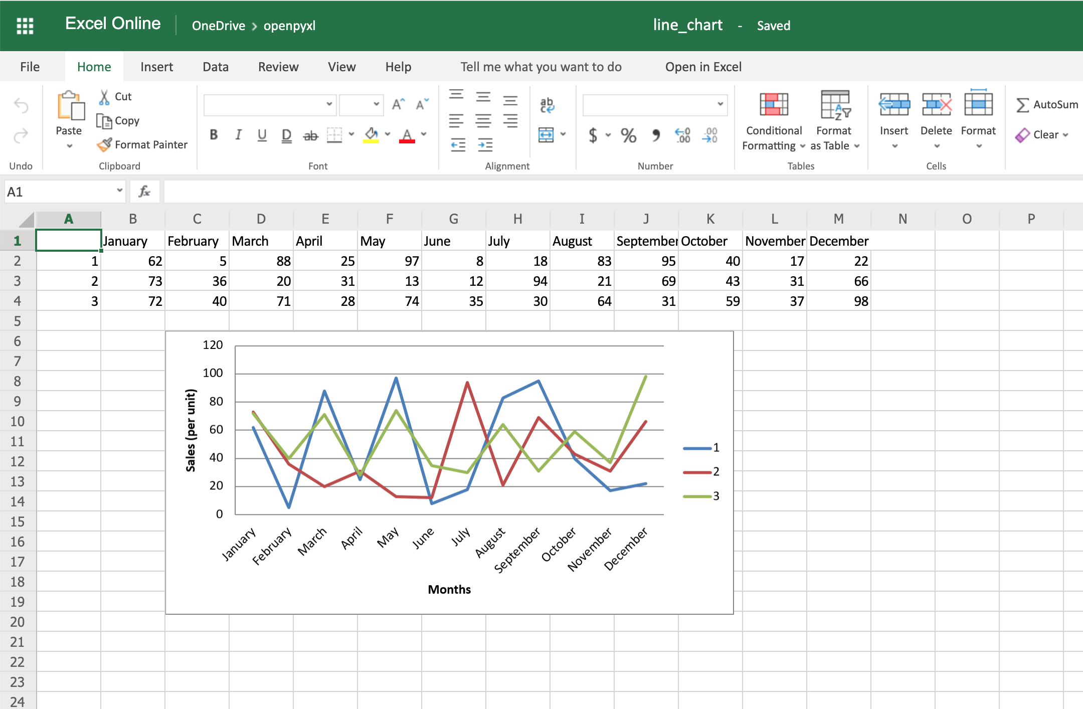
As you can see, small changes like the above make reading your chart a much easier and quicker task.
There is also a way to style your chart by using Excel’s default ChartStyle property. In this case, you have to choose a number between 1 and 48. Depending on your choice, the colors of your chart change as well:
# You can play with this by choosing any number between 1 and 48
chart.style = 24
With the style selected above, all lines have some shade of orange:
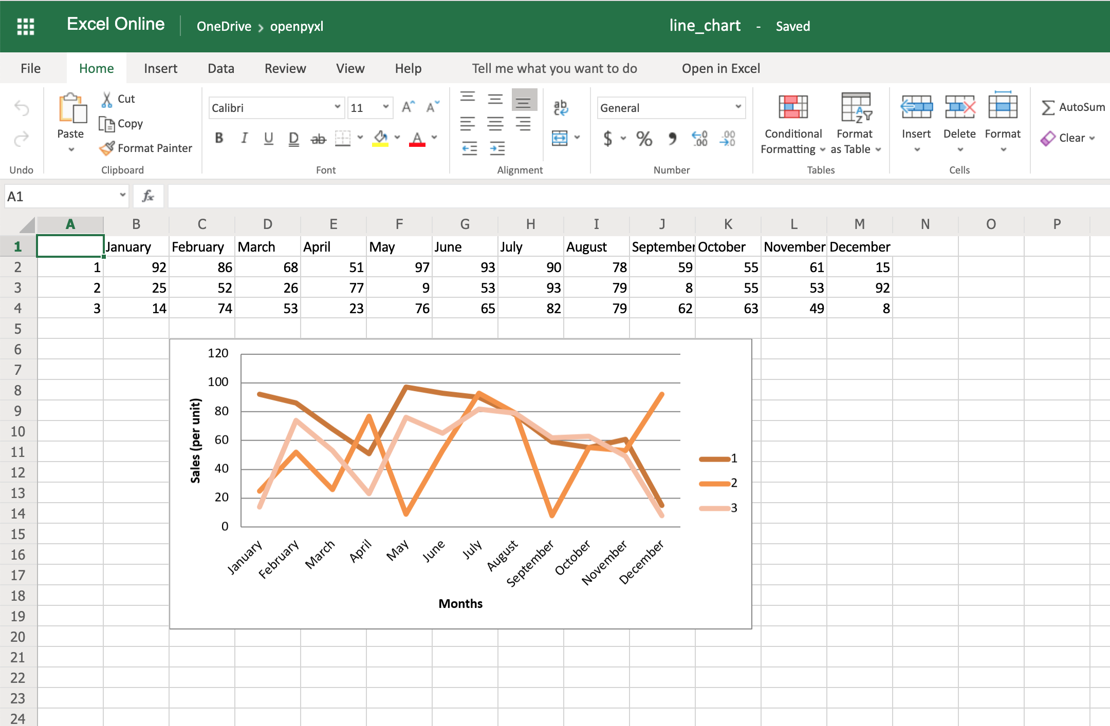
There is no clear documentation on what each style number looks like, but this spreadsheet has a few examples of the styles available.
Here’s the full code used to generate the line chart with categories, axis titles, and style:
import random
from openpyxl import Workbook
from openpyxl.chart import LineChart, Reference

workbook = Workbook()
sheet = workbook.active

# Let's create some sample sales data
rows = [
    ["", "January", "February", "March", "April",
    "May", "June", "July", "August", "September",
     "October", "November", "December"],
    [1, ],
    [2, ],
    [3, ],
]

for row in rows:
    sheet.append(row)

for row in sheet.iter_rows(min_row=2,
                           max_row=4,
                           min_col=2,
                           max_col=13):
    for cell in row:
        cell.value = random.randrange(5, 100)

# Create a LineChart and add the main data
chart = LineChart()
data = Reference(worksheet=sheet,
                           min_row=2,
                           max_row=4,
                           min_col=1,
                           max_col=13)
chart.add_data(data, titles_from_data=True, from_rows=True)

# Add categories to the chart
cats = Reference(worksheet=sheet,
                 min_row=1,
                 max_row=1,
                 min_col=2,
                 max_col=13)
chart.set_categories(cats)

# Rename the X and Y Axis
chart.x_axis.title = "Months"
chart.y_axis.title = "Sales (per unit)"

# Apply a specific Style
chart.style = 24

# Save!
sheet.add_chart(chart, "C6")
workbook.save("line_chart.xlsx")
There are a lot more chart types and customization you can apply, so be sure to check out the package documentation on this if you need some specific formatting.
Convert Python Classes to Excel Spreadsheet
You already saw how to convert an Excel spreadsheet’s data into Python classes, but now let’s do the opposite.
Let’s imagine you have a database and are using some Object-Relational Mapping (ORM) to map DB objects into Python classes. Now, you want to export those same objects into a spreadsheet.
Let’s assume the following data classes to represent the data coming from your database regarding product sales:
from dataclasses import dataclass
from typing import List

@dataclass
class Sale:
    quantity: int

@dataclass
class Product:
    id: str
    name: str
    sales: List[Sale]
Now, let’s generate some random data, assuming the above classes are stored in a db_classes.py file:
 1import random
 2
 3# Ignore these for now. You'll use them in a sec ;)
 4from openpyxl import Workbook
 5from openpyxl.chart import LineChart, Reference
 6
 7from db_classes import Product, Sale
 8
 9products = []
10
11# Let's create 5 products
12for idx in range(1, 6):
13    sales = []
14
15    # Create 5 months of sales
16    for _ in range(5):
17        sale = Sale(quantity=random.randrange(5, 100))
18        sales.append(sale)
19
20    product = Product(id=str(idx),
21                      name="Product %s" % idx,
22                      sales=sales)
23    products.append(product)
By running this piece of code, you should get 5 products with 5 months of sales with a random quantity of sales for each month.
Now, to convert this into a spreadsheet, you need to iterate over the data and append it to the spreadsheet:
25workbook = Workbook()
26sheet = workbook.active
27
28# Append column names first
29sheet.append(["Product ID", "Product Name", "Month 1",
30              "Month 2", "Month 3", "Month 4", "Month 5"])
31
32# Append the data
33for product in products:
34    data = [product.id, product.name]
35    for sale in product.sales:
36        data.append(sale.quantity)
37    sheet.append(data)
That’s it. That should allow you to create a spreadsheet with some data coming from your database.
However, why not use some of that cool knowledge you gained recently to add a chart as well to display that data more visually?
All right, then you could probably do something like this:
38chart = LineChart()
39data = Reference(worksheet=sheet,
40                 min_row=2,
41                 max_row=6,
42                 min_col=2,
43                 max_col=7)
44
45chart.add_data(data, titles_from_data=True, from_rows=True)
46sheet.add_chart(chart, "B8")
47
48cats = Reference(worksheet=sheet,
49                 min_row=1,
50                 max_row=1,
51                 min_col=3,
52                 max_col=7)
53chart.set_categories(cats)
54
55chart.x_axis.title = "Months"
56chart.y_axis.title = "Sales (per unit)"
57
58workbook.save(filename="oop_sample.xlsx")
Now we’re talking! Here’s a spreadsheet generated from database objects and with a chart and everything:
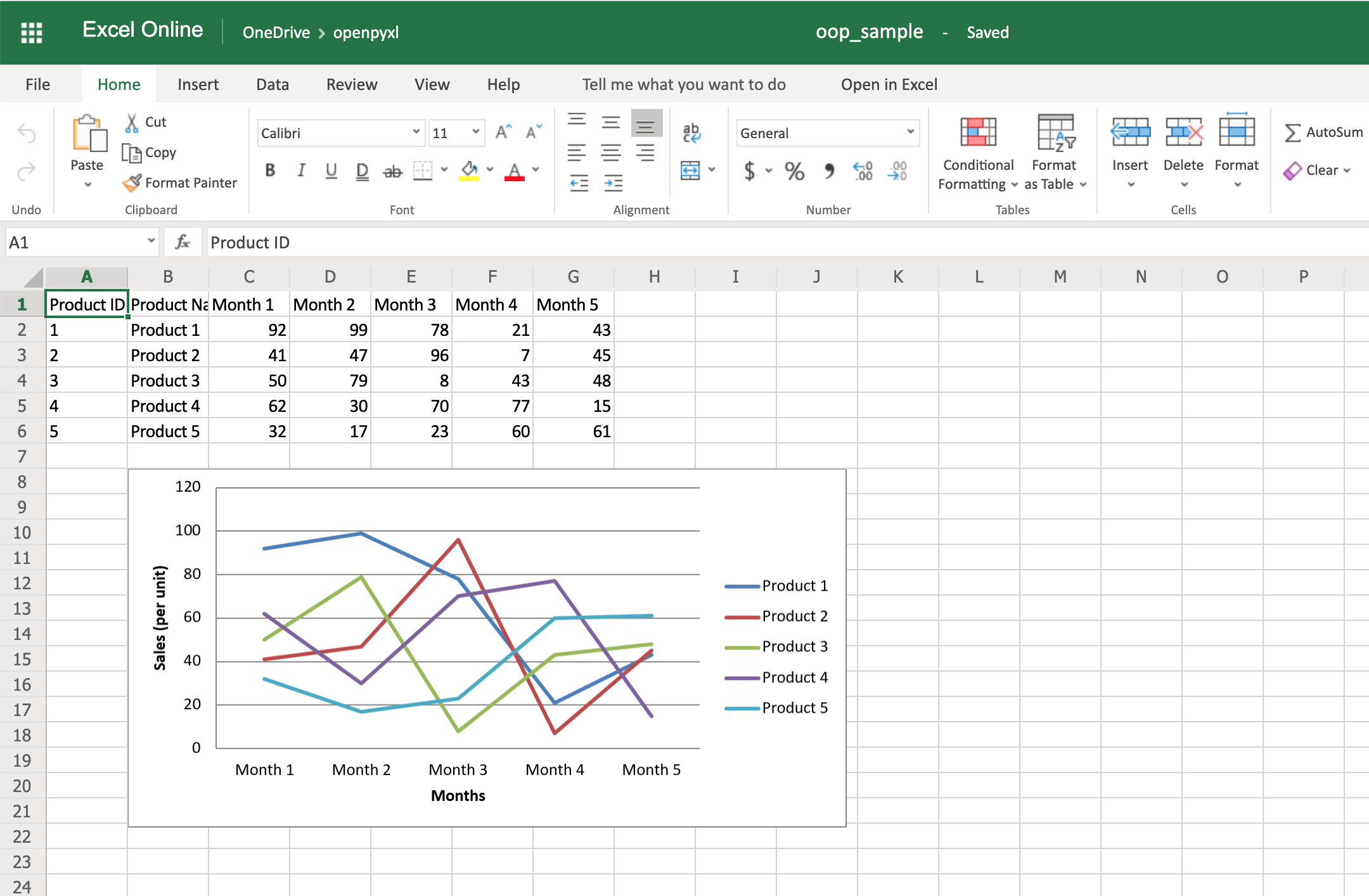
That’s a great way for you to wrap up your new knowledge of charts!
Bonus: Working With Pandas
Even though you can use Pandas to handle Excel files, there are few things that you either can’t accomplish with Pandas or that you’d be better off just using openpyxl directly.
For example, some of the advantages of using openpyxl are the ability to easily customize your spreadsheet with styles, conditional formatting, and such.
But guess what, you don’t have to worry about picking. In fact, openpyxl has support for both converting data from a Pandas DataFrame into a workbook or the opposite, converting an openpyxl workbook into a Pandas DataFrame.
First things first, remember to install the pandas package:
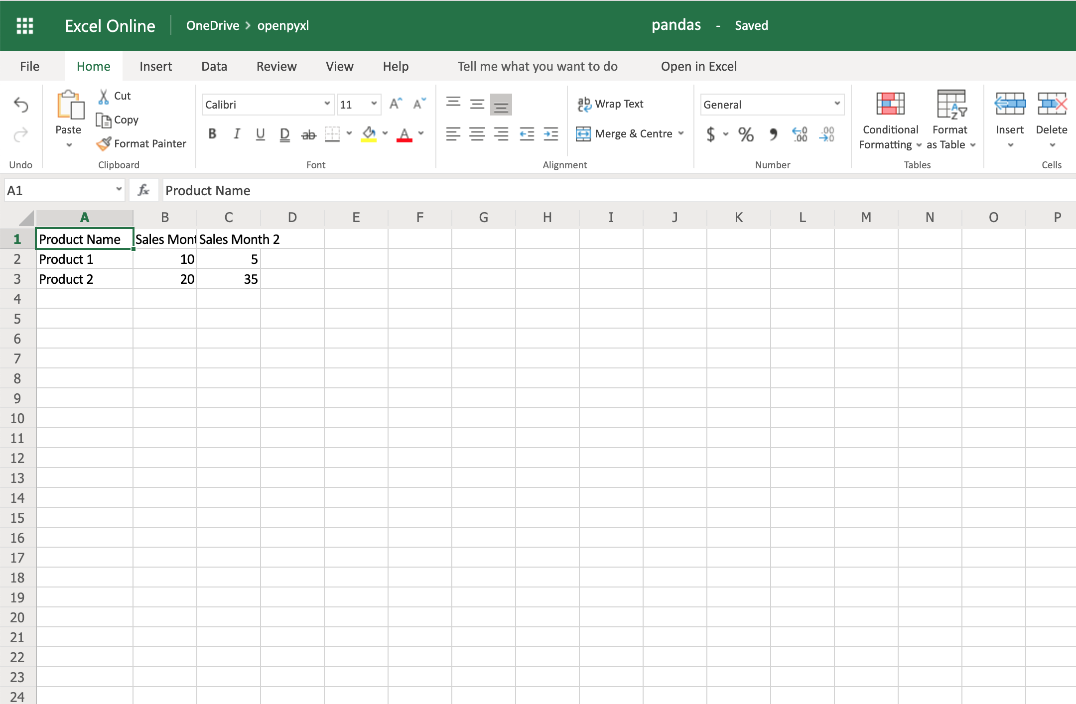
Then, let’s create a sample DataFrame:
 1import pandas as pd
 2
 3data = {
 4    "Product Name": ["Product 1", "Product 2"],
 5    "Sales Month 1": [10, 20],
 6    "Sales Month 2": [5, 35],
 7}
 8df = pd.DataFrame(data)
Now that you have some data, you can use .dataframe_to_rows() to convert it from a DataFrame into a worksheet:
10from openpyxl import Workbook
11from openpyxl.utils.dataframe import dataframe_to_rows
12
13workbook = Workbook()
14sheet = workbook.active
15
16for row in dataframe_to_rows(df, index=False, header=True):
17    sheet.append(row)
18
19workbook.save("pandas.xlsx")
You should see a spreadsheet that looks like this:
If you want to add the DataFrame’s index, you can change index=True, and it adds each row’s index into your spreadsheet.
On the other hand, if you want to convert a spreadsheet into a DataFrame, you can also do it in a very straightforward way like so:
import pandas as pd
from openpyxl import load_workbook

workbook = load_workbook(filename="sample.xlsx")
sheet = workbook.active

values = sheet.values
df = pd.DataFrame(values)
Alternatively, if you want to add the correct headers and use the review ID as the index, for example, then you can also do it like this instead:
import pandas as pd
from openpyxl import load_workbook
from mapping import REVIEW_ID

workbook = load_workbook(filename="sample.xlsx")
sheet = workbook.active

data = sheet.values

# Set the first row as the columns for the DataFrame
cols = next(data)
data = list(data)

# Set the field "review_id" as the indexes for each row
idx = [row[REVIEW_ID] for row in data]

df = pd.DataFrame(data, index=idx, columns=cols)
Using indexes and columns allows you to access data from your DataFrame easily:
>>>
>>> df.columns
Index(['marketplace', 'customer_id', 'review_id', 'product_id',
       'product_parent', 'product_title', 'product_category', 'star_rating',
       'helpful_votes', 'total_votes', 'vine', 'verified_purchase',
       'review_headline', 'review_body', 'review_date'],
      dtype='object')

>>> # Get first 10 reviews' star rating
>>> df["star_rating"][:10]
R3O9SGZBVQBV76    5
RKH8BNC3L5DLF     5
R2HLE8WKZSU3NL    2
R31U3UH5AZ42LL    5
R2SV659OUJ945Y    4
RA51CP8TR5A2L     5
RB2Q7DLDN6TH6     5
R2RHFJV0UYBK3Y    1
R2Z6JOQ94LFHEP    5
RX27XIIWY5JPB     4
Name: star_rating, dtype: int64

>>> # Grab review with id "R2EQL1V1L6E0C9", using the index
>>> df.loc["R2EQL1V1L6E0C9"]
marketplace               US
customer_id         15305006
review_id     R2EQL1V1L6E0C9
product_id        B004LURNO6
product_parent     892860326
review_headline   Five Stars
review_body          Love it
review_date       2015-08-31
Name: R2EQL1V1L6E0C9, dtype: object
There you go, whether you want to use openpyxl to prettify your Pandas dataset or use Pandas to do some hardcore algebra, you now know how to switch between both packages.
Conclusion
Phew, after that long read, you now know how to work with spreadsheets in Python! You can rely on openpyxl, your trustworthy companion, to:
- Extract valuable information from spreadsheets in a Pythonic manner
- Create your own spreadsheets, no matter the complexity level
- Add cool features such as conditional formatting or charts to your spreadsheets
There are a few other things you can do with openpyxl that might not have been covered in this tutorial, but you can always check the package’s official documentation website to learn more about it. You can even venture into checking its source code and improving the package further.
Feel free to leave any comments below if you have any questions, or if there’s any section you’d love to hear more about.
Watch Now This tutorial has a related video course created by the Real Python team. Watch it together with the written tutorial to deepen your understanding: Editing Excel Spreadsheets in Python With openpyxl
Python XlsxWriter — Overview
XlsxWriter is a Python module for creating spreadsheet files in Excel 2007 (XLSX) format that uses open XML standards. XlsxWriter module has been developed by John McNamara. Its earliest version (0.0.1) was released in 2013. The latest version 3.0.2 was released in November 2021. The latest version requires Python 3.4 or above.
XlsxWriter Features
Some of the important features of XlsxWriter include −
-
Files created by XlsxWriter are 100% compatible with Excel XLSX files.
-
XlsxWriter provides full formatting features such as Merged cells, Defined names, conditional formatting, etc.
-
XlsxWriter allows programmatically inserting charts in XLSX files.
-
Autofilters can be set using XlsxWriter.
-
XlsxWriter supports Data validation and drop-down lists.
-
Using XlsxWriter, it is possible to insert PNG/JPEG/GIF/BMP/WMF/EMF images.
-
With XlsxWriter, Excel spreadsheet can be integrated with Pandas library.
-
XlsxWriter also provides support for adding Macros.
-
XlsxWriter has a Memory optimization mode for writing large files.
Python XlsxWriter — Environment Setup
Installing XlsxWriter using PIP
The easiest and recommended method of installing XlsxWriter is to use PIP installer. Use the following command to install XlsxWriter (preferably in a virtual environment).
pip3 install xlsxwriter
Installing from a Tarball
Another option is to install XlsxWriter from its source code, hosted at https://github.com/jmcnamara/XlsxWriter/. Download the latest source tarball and install the library using the following commands −
$ curl -O -L http://github.com/jmcnamara/XlsxWriter/archive/main.tar.gz

$ tar zxvf main.tar.gz
$ cd XlsxWriter-main/
$ python setup.py install
Cloning from GitHub
You may also clone the GitHub repository and install from it.
$ git clone https://github.com/jmcnamara/XlsxWriter.git

$ cd XlsxWriter
$ python setup.py install
To confirm that XlsxWriter is installed properly, check its version from the Python prompt −
>>> import xlsxwriter
>>> xlsxwriter.__version__
'3.0.2'
Python XlsxWriter — Hello World
Getting Started
The first program to test if the module/library works correctly is often to write Hello world message. The following program creates a file with .XLSX extension. An object of the Workbook class in the xlsxwriter module corresponds to the spreadsheet file in the current working directory.
wb = xlsxwriter.Workbook('hello.xlsx')
Next, call the add_worksheet() method of the Workbook object to insert a new worksheet in it.
ws = wb.add_worksheet()
We can now add the Hello World string at A1 cell by invoking the write() method of the worksheet object. It needs two parameters: the cell address and the string.
ws.write('A1', 'Hello world')
Example
The complete code of hello.py is as follows −
import xlsxwriter
wb = xlsxwriter.Workbook('hello.xlsx')
ws = wb.add_worksheet()
ws.write('A1', 'Hello world')
wb.close()
Output
After the above code is executed, hello.xlsx file will be created in the current working directory. You can now open it using Excel software.
Python XlsxWriter — Important Classes
The XlsxWriter library comprises of following classes. All the methods defined in these classes allow different operations to be done programmatically on the XLSX file. The classes are −
- Workbook class
- Worksheet class
- Format class
- Chart class
- Chartsheet class
- Exception class
Workbook Class
This is the main class exposed by the XlsxWriter module and it is the only class that you will need to instantiate directly. It represents the Excel file as it is written on a disk.
wb=xlsxwriter.Workbook('filename.xlsx')
The Workbook class defines the following methods −
| Sr.No | Workbook Class & Description |
|---|---|
| 1 |
add_worksheet() Adds a new worksheet to a workbook. |
| 2 |
add_format() Used to create new Format objects which are used to apply formatting to a cell. |
| 3 |
add_chart() Creates a new chart object that can be inserted into a worksheet via the insert_chart() Worksheet method |
| 4 |
add_chartsheet() Adds a new chartsheet to a workbook. |
| 5 |
close() Closes the Workbook object and write the XLSX file. |
| 6 |
define_name() Creates a defined name in the workbook to use as a variable. |
| 7 |
add_vba_project() Used to add macros or functions to a workbook using a binary VBA project file. |
| 8 |
worksheets() Returns a list of the worksheets in a workbook. |
Worksheet Class
The worksheet class represents an Excel worksheet. An object of this class handles operations such as writing data to cells or formatting worksheet layout. It is created by calling the add_worksheet() method from a Workbook() object.
The Worksheet object has access to the following methods −
|
write() |
Writes generic data to a worksheet cell. Parameters −
Returns −
|
|
write_string() |
Writes a string to the cell specified by row and column. Parameters −
Returns −
|
|
write_number() |
Writes numeric types to the cell specified by row and column. Parameters −
Returns −
|
|
write_formula() |
Writes a formula or function to the cell specified by row and column. Parameters −
Returns −
|
|
insert_image() |
Used to insert an image into a worksheet. The image can be in PNG, JPEG, GIF, BMP, WMF or EMF format. Parameters −
Returns −
|
|
insert_chart() |
Used to insert a chart into a worksheet. A chart object is created via the Workbook add_chart() method. Parameters −
|
|
conditional_format() |
Used to add formatting to a cell or range of cells based on user-defined criteria. Parameters −
Returns −
|
|
add_table() |
Used to group a range of cells into an Excel Table. Parameters −
|
|
autofilter() |
Set the auto-filter area in the worksheet. It adds drop down lists to the headers of a 2D range of worksheet data. User can filter the data based on simple criteria. Parameters −
|
Format Class
Format objects are created by calling the workbook add_format() method. Methods and properties available to this object are related to fonts, colors, patterns, borders, alignment and number formatting.
Font formatting methods and properties −
| Method Name | Description | Property |
|---|---|---|
| set_font_name() | Font type | ‘font_name’ |
| set_font_size() | Font size | ‘font_size’ |
| set_font_color() | Font color | ‘font_color’ |
| set_bold() | Bold | ‘bold’ |
| set_italic() | Italic | ‘italic’ |
| set_underline() | Underline | ‘underline’ |
| set_font_strikeout() | Strikeout | ‘font_strikeout’ |
| set_font_script() | Super/Subscript | ‘font_script’ |
Alignment formatting methods and properties
| Method Name | Description | Property |
|---|---|---|
| set_align() | Horizontal align | ‘align’ |
| set_align() | Vertical align | ‘valign’ |
| set_rotation() | Rotation | ‘rotation’ |
| set_text_wrap() | Text wrap | ‘text_wrap’ |
| set_reading_order() | Reading order | ‘reading_order’ |
| set_text_justlast() | Justify last | ‘text_justlast’ |
| set_center_across() | Center across | ‘center_across’ |
| set_indent() | Indentation | ‘indent’ |
| set_shrink() | Shrink to fit | ‘shrink’ |
Chart Class
A chart object is created via the add_chart() method of the Workbook object where the chart type is specified.
chart = workbook.add_chart({'type': 'column'})
The chart object is inserted in the worksheet by calling insert_chart() method.
worksheet.insert_chart('A7', chart)
XlxsWriter supports the following chart types −
-
area − Creates an Area (filled line) style chart.
-
bar − Creates a Bar style (transposed histogram) chart.
-
column − Creates a column style (histogram) chart.
-
line − Creates a Line style chart.
-
pie − Creates a Pie style chart.
-
doughnut − Creates a Doughnut style chart.
-
scatter − Creates a Scatter style chart.
-
stock − Creates a Stock style chart.
-
radar − Creates a Radar style chart.
The Chart class defines the following methods −
|
add_series(options) |
Add a data series to a chart. Following properties can be given −
|
|
set_x_axis(options) |
Set the chart X-axis options including
|
|
set_y_axis(options) |
Set the chart Y-axis options including −
|
|
set_size() |
This method is used to set the dimensions of the chart. The size of the chart can be modified by setting the width and height or by setting the x_scale and y_scale. |
|
set_title(options) |
Set the chart title options. Parameters −
|
|
set_legend() |
This method formats the chart legends with the following properties −
|
Chartsheet Class
A chartsheet in a XLSX file is a worksheet that only contains a chart and no other data. a new chartsheet object is created by calling the add_chartsheet() method from a Workbook object −
chartsheet = workbook.add_chartsheet()
Some functionalities of the Chartsheet class are similar to that of data Worksheets such as tab selection, headers, footers, margins, and print properties. However, its primary purpose is to display a single chart, whereas an ordinary data worksheet can have one or more embedded charts.
The data for the chartsheet chart must be present on a separate worksheet. Hence it is always created along with at least one data worksheet, using set_chart() method.
chartsheet = workbook.add_chartsheet()
chart = workbook.add_chart({'type': 'column'})
chartsheet.set_chart(chart)
Remember that a Chartsheet can contain only one chart.
Example
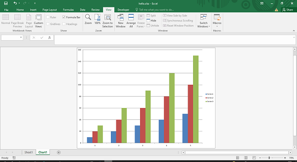
The following code writes the data series in the worksheet names sheet1 but opens a new chartsheet to add a column chart based on the data in sheet1.
import xlsxwriter

wb = xlsxwriter.Workbook('hello.xlsx')
worksheet = wb.add_worksheet()

cs = wb.add_chartsheet()
chart = wb.add_chart({'type': 'column'})

data = [
   [10, 20, 30, 40, 50],
   [20, 40, 60, 80, 100],
   [30, 60, 90, 120, 150],
]
worksheet.write_column('A1', data[0])
worksheet.write_column('B1', data[1])
worksheet.write_column('C1', data[2])

chart.add_series({'values': '=Sheet1!$A$1:$A$5'})
chart.add_series({'values': '=Sheet1!$B$1:$B$5'})
chart.add_series({'values': '=Sheet1!$C$1:$C$5'})

cs.set_chart(chart)
cs.activate()

wb.close()
Output
Exception Class
XlsxWriter identifies various run-time errors or exceptions which can be trapped using Python’s error handling technique so as to avoid corruption of Excel files. The Exception classes in XlsxWriter are as follows −
| Sr.No | Exception Classes & Description |
|---|---|
| 1 |
XlsxWriterException Base exception for XlsxWriter. |
| 2 |
XlsxFileError Base exception for all file related errors. |
| 3 |
XlsxInputError Base exception for all input data related errors. |
| 4 |
FileCreateError Occurs if there is a file permission error, or IO error, when writing the xlsx file to disk or if the file is already open in Excel. |
| 5 |
UndefinedImageSize Raised with insert_image() method if the image doesn’t contain height or width information. The exception is raised during Workbook close(). |
| 6 |
UnsupportedImageFormat Raised if the image isn’t one of the supported file formats: PNG, JPEG, GIF, BMP, WMF or EMF. |
| 7 |
EmptyChartSeries This exception occurs when a chart is added to a worksheet without a data series. |
| 8 |
InvalidWorksheetName if a worksheet name is too long or contains invalid characters. |
| 9 |
DuplicateWorksheetName This exception is raised when a worksheet name is already present. |
Exception FileCreateError
Assuming that a workbook named hello.xlsx is already opened using Excel app, then the following code will raise a FileCreateError −
import xlsxwriter
workbook = xlsxwriter.Workbook('hello.xlsx')
worksheet = workbook.add_worksheet()
workbook.close()
When this program is run, the error message is displayed as below −
PermissionError: [Errno 13] Permission denied: 'hello.xlsx'
During handling of the above exception, another exception occurred:
Traceback (most recent call last):
   File "hello.py", line 4, in <module>
   workbook.close()
File "e:xlsxenvlibsite-packagesxlsxwriterworkbook.py", line 326, in close
   raise FileCreateError(e)
xlsxwriter.exceptions.FileCreateError: [Errno 13] Permission denied: 'hello.xlsx'
Handling the Exception
We can use Python’s exception handling mechanism for this purpose.
import xlsxwriter
try:
   workbook = xlsxwriter.Workbook('hello.xlsx')
   worksheet = workbook.add_worksheet()
   workbook.close()
except:
   print ("The file is already open")
Now the custom error message will be displayed.
(xlsxenv) E:xlsxenv>python ex34.py
The file is already open
Exception EmptyChartSeries
Another situation of an exception being raised when a chart is added with a data series.
import xlsxwriter
workbook = xlsxwriter.Workbook('hello.xlsx')
worksheet = workbook.add_worksheet()
chart = workbook.add_chart({'type': 'column'})
worksheet.insert_chart('A7', chart)
workbook.close()
This leads to EmptyChartSeries exception −
xlsxwriter.exceptions.EmptyChartSeries: Chart1 must contain at least one data series.
Python XlsxWriter — Cell Notation & Ranges
Each worksheet in a workbook is a grid of a large number of cells, each of which can store one piece of data — either value or formula. Each Cell in the grid is identified by its row and column number.
In Excel’s standard cell addressing, columns are identified by alphabets, A, B, C, …., Z, AA, AB etc., and rows are numbered starting from 1.
The address of each cell is alphanumeric, where the alphabetic part corresponds to the column and number corresponding to the row. For example, the address «C5» points to the cell in column «C» and row number «5».
Cell Notations
The standard Excel uses alphanumeric sequence of column letter and 1-based row. XlsxWriter supports the standard Excel notation (A1 notation) as well as Row-column notation which uses a zero based index for both row and column.
Example
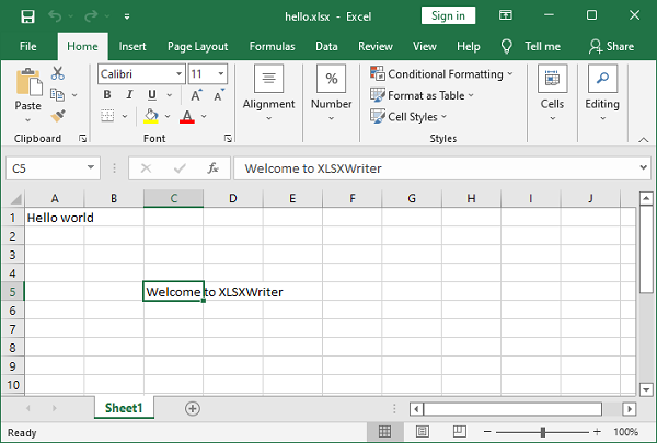
In the following example, a string ‘Hello world’ is written into A1 cell using Excel’s standard cell address, while ‘Welcome to XLSXWriter’ is written into cell C5 using row-column notation.
import xlsxwriter
wb = xlsxwriter.Workbook('hello.xlsx')
ws = wb.add_worksheet()
ws.write('A1', 'Hello world')           # A1 notation
ws.write(4,2,"Welcome to XLSXWriter")   # Row-column notation
wb.close()
Output
Open the hello.xlsx file using Excel software.
The numbered row-column notation is especially useful when referring to the cells programmatically. In the following code data in a list of lists has to be written to a range of cells in a worksheet. This is achieved by two nested loops, the outer representing the row numbers and the inner loop for column numbers.
data = [
   ['Name', 'Physics', 'Chemistry', 'Maths', 'Total'],
   ['Ravi', 60, 70, 80],
   ['Kiran', 65, 75, 85],
   ['Karishma', 55, 65, 75],
]
for row in range(len(data)):
   for col in range(len(data[row])):
      ws.write(row, col, data[row][col])
The same result can be achieved by using write_row() method of the worksheet object used in the code below −
for row in range(len(data)):
   ws.write_row(6+row,0, data[row])
The worksheet object has add_table() method that writes the data to a range and converts into Excel range, displaying autofilter dropdown arrows in the top row.
ws.add_table('G6:J9', {'data': data, 'header_row':True})
Example
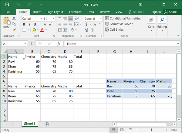
The output of all the three codes above can be verified by the following code and displayed in the following figure −
import xlsxwriter

wb = xlsxwriter.Workbook('ex1.xlsx')
ws = wb.add_worksheet()

data = [
   ['Name', 'Physics', 'Chemistry', 'Maths', 'Total'],
   ['Ravi', 60, 70, 80],
   ['Kiran', 65, 75, 85],
   ['Karishma', 55, 65, 75],
]
for row in range(len(data)):
   for col in range(len(data[row])):
      ws.write(row, col, data[row][col])

for row in range(len(data)):
   ws.write_row(6+row,0, data[row])

ws.add_table('G6:J9', {'data': data, 'header_row':False})

wb.close()
Output
Execute the above program and open the ex1.xlsx using Excel software.
Python XlsxWriter — Defined Names
In Excel, it is possible to identify a cell, a formula, or a range of cells by user-defined name, which can be used as a variable used to make the definition of formula easy to understand. This can be achieved using the define_name() method of the Workbook class.
In the following code snippet, we have a range of cells consisting of numbers. This range has been given a name as marks.
data=['marks',50,60,70, 'Total']
ws.write_row('A1', data)
wb.define_name('marks', '=Sheet1!$A$1:$E$1')
If the name is assigned to a range of cells, the second argument of define_name() method is a string with the name of the sheet followed by «!» symbol and then the range of cells using the absolute addressing scheme. In this case, the range A1:E1 in sheet1 is named as marks.
This name can be used in any formula. For example, we calculate the sum of numbers in the range identified by the name marks.
ws.write('F1', '=sum(marks)')
We can also use the named cell in the write_formula() method. In the following code, this method is used to calculate interest on the amount where the rate is a defined_name.
ws.write('B5', 10)
wb.define_name('rate', '=sheet1!$B$5')

ws.write_row('A5', ['Rate', 10])

data=['Amount',1000, 2000, 3000]
ws.write_column('A6', data)
ws.write('B6', 'Interest')
for row in range(6,9):
   ws.write_formula(row, 1, '= rate*$A{}/100'.format(row+1))
We can also use write_array_formula() method instead of the loop in the above code −
ws.write_array_formula('D7:D9' , '{=rate/100*(A7:A9)}')
Example
The complete code using define_name() method is given below −
import xlsxwriter

wb = xlsxwriter.Workbook('ex2.xlsx')
ws = wb.add_worksheet()

data = ['marks',50,60,70, 'Total']
ws.write_row('A1', data)
wb.define_name('marks', '=Sheet1!$A$1:$E$1')
ws.write('F1', '=sum(marks)')

ws.write('B5', 10)
wb.define_name('rate', '=sheet1!$B$5')

ws.write_row('A5', ['Rate', 10])

data=['Amount',1000, 2000, 3000]
ws.write_column('A6', data)
ws.write('B6', 'Interest')

for row in range(6,9):
   ws.write_formula(row, 1, '= rate*$A{}/100'.format(row+1))

wb.close()
Output
Run the above program and open ex2.xlsx with Excel.
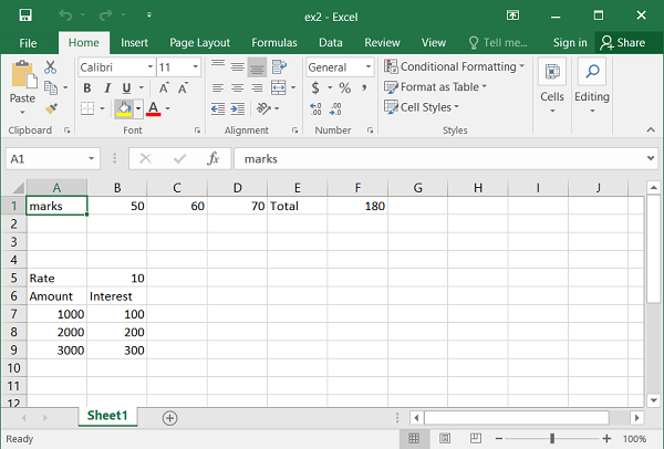
Python XlsxWriter — Formula & Function
The Worksheet class offers three methods for using formulas.
- write_formula()
- write_array_formula()
- write_dynamic_array_formula()
All these methods are used to assign formula as well as function to a cell.
The write_formula() Method
The write_formula() method requires the address of the cell, and a string containing a valid Excel formula. Inside the formula string, only the A1 style address notation is accepted. However, the cell address argument can be either standard Excel type or zero based row and column number notation.
Example
In the example below, various statements use write_formula() method. The first uses a standard Excel notation to assign a formula. The second statement uses row and column number to specify the address of the target cell in which the formula is set. In the third example, the IF() function is assigned to G2 cell.
import xlsxwriter

wb = xlsxwriter.Workbook('hello.xlsx')
ws = wb.add_worksheet()

data=[
   ['Name', 'Phy', 'Che', 'Maths', 'Total', 'percent', 'Result' ],
   ['Arvind', 50,60,70]
]
ws.write_row('A1', data[0])
ws.write_row('A2', data[1])
ws.write_formula('E2', '=B2+C2+D2')
ws.write_formula(1,5, '=E2*100/300')
ws.write_formula('G2', '=IF(F2>=50, "PASS","FAIL")')

wb.close()
Output
The Excel file shows the following result −
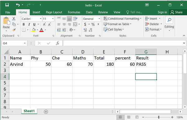
The write_array_formula() Method
The write_array_formula() method is used to extend the formula over a range. In Excel, an array formula performs a calculation on a set of values. It may return a single value or a range of values.
An array formula is indicated by a pair of braces around the formula − {=SUM(A1:B1*A2:B2)}. The range can be either specified by row and column numbers of first and last cell in the range (such as 0,0, 2,2) or by the string representation ‘A1:C2’.
Example
In the following example, array formulas are used for columns E, F and G to calculate total, percent and result from marks in the range B2:D4.
import xlsxwriter
wb = xlsxwriter.Workbook('hello.xlsx')
ws = wb.add_worksheet()

data=[
   ['Name', 'Phy', 'Che', 'Maths', 'Total', 'percent', 'Result'],
   ['Arvind', 50,60,70],
   ['Amar', 55,65,75],
   ['Asha', 75,85,80]
]

for row in range(len(data)):
   ws.write_row(row,0, data[row])

ws.write_array_formula('E2:E4', '{=B2:B4+C2:C4+D2:D4}')
ws.write_array_formula(1,5,3,5, '{=(E2:E4)*100/300}')
ws.write_array_formula('G2:G4', '{=IF((F2:F4)>=50, "PASS","FAIL")}')

wb.close()
Output
Here is how the worksheet appears when opened using MS Excel −
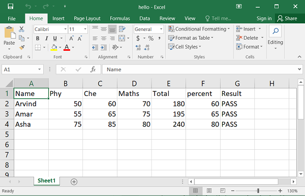
The write_dynamic_array_data() Method
The write_dynamic_array_data() method writes an dynamic array formula to a cell range. The concept of dynamic arrays has been introduced in EXCEL’s 365 version, and some new functions that leverage the advantage of dynamic arrays have been introduced. These functions are −
| Sr.No | Functions & Description |
|---|---|
| 1 |
FILTER Filter data and return matching records |
| 2 |
RANDARRAY Generate array of random numbers |
| 3 |
SEQUENCE Generate array of sequential numbers |
| 4 |
SORT Sort range by column |
| 5 |
SORTBY Sort range by another range or array |
| 6 |
UNIQUE Extract unique values from a list or range |
| 7 |
XLOOKUP replacement for VLOOKUP |
| 8 |
XMATCH replacement for the MATCH function |
Dynamic arrays are ranges of return values whose size can change based on the results. For example, a function such as FILTER() returns an array of values that can vary in size depending on the filter results.
Example
In the example below, the data range is A1:D17. The filter function uses this range and the criteria range is C1:C17, in which the product names are given. The FILTER() function results in a dynamic array as the number of rows satisfying the criteria may change.
import xlsxwriter

wb = xlsxwriter.Workbook('hello.xlsx')
ws = wb.add_worksheet()

data = (
   ['Region', 'SalesRep', 'Product', 'Units'],
   ['East',   'Tom',      'Apple',    6380],
   ['West',   'Fred',     'Grape',    5619],
   ['North',  'Amy',      'Pear',     4565],
   ['South',  'Sal',      'Banana',   5323],
   ['East',   'Fritz',    'Apple',    4394],
   ['West',   'Sravan',   'Grape',    7195],
   ['North',  'Xi',       'Pear',     5231],
   ['South',  'Hector',   'Banana',   2427],
   ['East',   'Tom',      'Banana',   4213],
   ['West',   'Fred',     'Pear',     3239],
   ['North',  'Amy',      'Grape',    6520],
   ['South',  'Sal',      'Apple',    1310],
   ['East',   'Fritz',    'Banana',   6274],
   ['West',   'Sravan',   'Pear',     4894],
   ['North',  'Xi',       'Grape',    7580],
   ['South',  'Hector',   'Apple',    9814])
for row in range(len(data)):
   ws.write_row(row,0, data[row])

ws.write_dynamic_array_formula('F1', '=FILTER(A1:D17,C1:C17="Apple")')
wb.close()
Output
Note that the formula string to write_dynamic_array_formula() need not contain curly brackets. The resultant hello.xlsx must be opened with Excel 365 app.
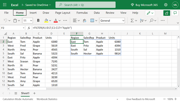
Python XlsxWriter — Date & Time
In Excel, dates are stored as real numbers so that they can be used in calculations. By default, January 1, 1900 (called as epoch) is treated 1, and hence January 28, 2022 corresponds to 44589. Similarly, the time is represented as the fractional part of the number, as the percentage of day. Hence, January 28, 2022 11.00 corresponds to 44589.45833.
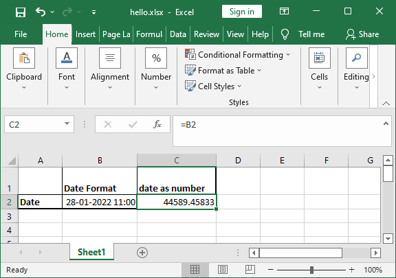
The set_num_format() Method
Since date or time in Excel is just like any other number, to display the number as a date you must apply an Excel number format to it. Use set_num_format() method of the Format object using appropriate formatting.
The following code snippet displays a number in «dd/mm/yy» format.
num = 44589
format1 = wb.add_format()
format1.set_num_format('dd/mm/yy')
ws.write('B2', num, format1)
The num_format Parameter
Alternatively, the num_format parameter of add_format() method can be set to the desired format.
format1 = wb.add_format({'num_format':'dd/mm/yy'})
ws.write('B2', num, format1)
Example
The following code shows the number in various date formats.
import xlsxwriter

wb = xlsxwriter.Workbook('hello.xlsx')
ws = wb.add_worksheet()

num=44589
ws.write('A1', num)

format2 = wb.add_format({'num_format': 'dd/mm/yy'})
ws.write('A2', num, format2)

format3 = wb.add_format({'num_format': 'mm/dd/yy'})
ws.write('A3', num, format3)

format4 = wb.add_format({'num_format': 'd-m-yyyy'})
ws.write('A4', num, format4)

format5 = wb.add_format({'num_format': 'dd/mm/yy hh:mm'})
ws.write('A5', num, format5)

format6 = wb.add_format({'num_format': 'd mmm yyyy'})
ws.write('A6', num, format6)

format7 = wb.add_format({'num_format': 'mmm d yyyy hh:mm AM/PM'})
ws.write('A7', num, format7)

wb.close()
Output
The worksheet looks like the following in Excel software −

write_datetime() and strptime()
The XlsxWriter’s Worksheet object also has write_datetime() method that is useful when handling date and time objects obtained with datetime module of Python’s standard library.
The strptime() method returns datetime object from a string parsed according to the given format. Some of the codes used to format the string are given below −
|
%a |
Abbreviated weekday name |
Sun, Mon |
|
%A |
Full weekday name |
Sunday, Monday |
|
%d |
Day of the month as a zero-padded decimal |
01, 02 |
|
%-d |
day of the month as decimal number |
1, 2.. |
|
%b |
Abbreviated month name |
Jan, Feb |
|
%m |
Month as a zero padded decimal number |
01, 02 |
|
%-m |
Month as a decimal number |
1, 2 |
|
%B |
Full month name |
January, February |
|
%y |
Year without century as a zero padded decimal number |
99, 00 |
|
%-y |
Year without century as a decimal number |
0, 99 |
|
%Y |
Year with century as a decimal number |
2022, 1999 |
|
%H |
Hour (24 hour clock) as a zero padded decimal number |
01, 23 |
|
%-H |
Hour (24 hour clock) as a decimal number |
1, 23 |
|
%I |
Hour (12 hour clock) as a zero padded decimal number |
01, 12 |
|
%-I |
Hour (12 hour clock) as a decimal number |
1, 12 |
|
%p |
locale’s AM or PM |
AM, PM |
|
%M |
Minute as a zero padded decimal number |
01, 59 |
|
%-M |
Minute as a decimal number |
1, 59 |
|
%S |
Second as a zero padded decimal number |
01, 59 |
|
%-S |
Second as a decimal number |
1, 59 |
|
%c |
locale’s appropriate date and time representation |
Mon Sep 30 07:06:05 2022 |
The strptime() method is used as follows −
>>> from datetime import datetime
>>> dt="Thu February 3 2022 11:35:5"
>>> code="%a %B %d %Y %H:%M:%S"
>>> datetime.strptime(dt, code)
datetime.datetime(2022, 2, 3, 11, 35, 5)
This datetime object can now be written into the worksheet with write_datetime() method.
Example
In the following example, the datetime object is written with different formats.
import xlsxwriter
from datetime import datetime
wb = xlsxwriter.Workbook('hello.xlsx')
worksheet = wb.add_worksheet()

dt="Thu February 3 2022 11:35:5"
code="%a %B %d %Y %H:%M:%S"
obj=datetime.strptime(dt, code)
date_formats = (
   'dd/mm/yy',
   'mm/dd/yy',
   'dd m yy',
   'd mm yy',
   'd mmm yy',
   'd mmmm yy',
   'd mmmm yyy',
   'd mmmm yyyy',
   'dd/mm/yy hh:mm',
   'dd/mm/yy hh:mm:ss',
   'dd/mm/yy hh:mm:ss.000',
   'hh:mm',
   'hh:mm:ss',
   'hh:mm:ss.000',
)
worksheet.write('A1', 'Formatted date')
worksheet.write('B1', 'Format')
row = 1

for fmt in date_formats:
   date_format = wb.add_format({'num_format': fmt, 'align': 'left'})
   worksheet.write_datetime(row, 0, obj, date_format)
   worksheet.write_string(row, 1, fmt)
   row += 1
wb.close()
Output
The worksheet appears as follows when opened with Excel.
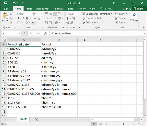
Python XlsxWriter — Tables
In MS Excel, a Table is a range of cells that has been grouped as a single entity. It can be referenced from formulas and has common formatting attributes. Several features such as column headers, autofilters, total rows, column formulas can be defined in a worksheet table.
The add_table() Method
The worksheet method add_table() is used to add a cell range as a table.
worksheet.add_table(first_row, first_col, last_row, last_col, options)
Both the methods, the standard ‘A1‘ or ‘Row/Column‘ notation are allowed for specifying the range. The add_table() method can take one or more of the following optional parameters. Note that except the range parameter, others are optional. If not given, an empty table is created.
Example
data
This parameter can be used to specify the data in the cells of the table. Look at the following example −
import xlsxwriter
wb = xlsxwriter.Workbook('hello.xlsx')
ws = wb.add_worksheet()

data = [
   ['Namrata',  75, 65, 80],
   ['Ravi',     60, 70, 80],
   ['Kiran',    65, 75, 85],
   ['Karishma', 55, 65, 75],
]
ws.add_table("A1:D4", {'data':data})

wb.close()
Output
Here’s the result −

header_row
This parameter can be used to turn on or off the header row in the table. It is on by default. The header row will contain default captions such as Column 1, Column 2, etc. You can set required captions by using the columns parameter.
Columns
Example
This property is used to set column captions.
import xlsxwriter

wb = xlsxwriter.Workbook('hello.xlsx')
ws = wb.add_worksheet()

data = [
   ['Namrata',  75, 65, 80],
   ['Ravi',     60, 70, 80],
   ['Kiran',    65, 75, 85],
   ['Karishma', 55, 65, 75],
]

ws.add_table("A1:D4",
{'data':data,
   'columns': [
   {'header': 'Name'},
   {'header': 'physics'},
   {'header': 'Chemistry'},
   {'header': 'Maths'}]
})
wb.close()
Output
The header row is now set as shown −
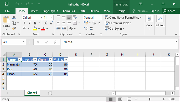
autofilter
This parameter is ON, by default. When set to OFF, the header row doesn’t show the dropdown arrows to set the filter criteria.
Name
In Excel worksheet, the tables are named as Table1, Table2, etc. The name parameter can be used to set the name of the table as required.
ws.add_table("A1:E4", {'data':data, 'name':'marklist'})
Formula
Column with a formula can be created by specifying formula sub-property in columns options.
Example
In the following example, the table’s name property is set to ‘marklist’. The formula for ‘Total’ column E performs sum of marks, and is assigned the value of formula sub-property.
import xlsxwriter

wb = xlsxwriter.Workbook('hello.xlsx')
ws = wb.add_worksheet()

data = [
   ['Namrata',  75, 65, 80],
   ['Ravi',     60, 70, 80],
   ['Kiran',    65, 75, 85],
   ['Karishma', 55, 65, 75],
]
formula = '=SUM(marklist[@[physics]:[Maths]])'
tbl = ws.add_table("A1:E5",
{'data': data,
   'autofilter': False,
   'name': 'marklist',
   'columns': [
      {'header': 'Name'},
      {'header': 'physics'},
      {'header': 'Chemistry'},
      {'header': 'Maths'},
      {'header': 'Total', 'formula': formula}
   ]
})
wb.close()
Output
When the above code is executed, the worksheet shows the Total column with the sum of marks.
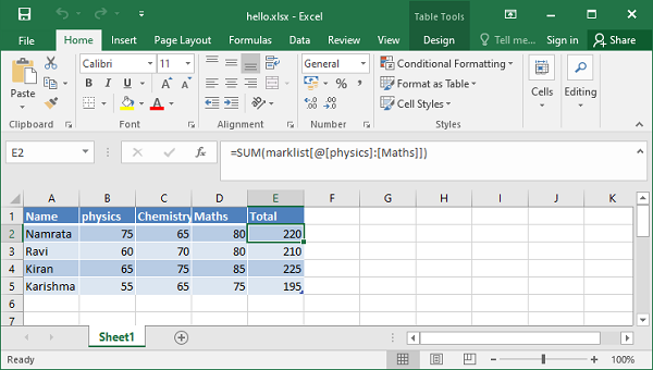
Python XlsxWriter — Applying Filter
In Excel, you can set filter on a tabular data based upon criteria using logical expressions. In XlsxWriter’s worksheet class, we have autofilter() method or the purpose. The mandatory argument to this method is the cell range. This creates drop-down selectors in the heading row. To apply some criteria, we have two methods available − filter_column() or filter_column_list().
Applying Filter Criteria for a Column
In the following example, the data in the range A1:D51 (i.e. cells 0,0 to 50,3) is used as the range argument for autofilter() method. The filter criteria ‘Region == East’ is set on 0th column (with Region heading) with filter_column() method.
Example
All the rows in the data range not meeting the filter criteria are hidden by setting hidden option to true for the set_row() method of the worksheet object.
import xlsxwriter

wb = xlsxwriter.Workbook('hello.xlsx')
ws = wb.add_worksheet()

data = (
   ['Region', 'SalesRep', 'Product', 'Units'],
   ['East',   'Tom',      'Apple',    6380],
   ['West',   'Fred',     'Grape',    5619],
   ['North',  'Amy',      'Pear',     4565],
   ['South',  'Sal',      'Banana',   5323],
   ['East',   'Fritz',    'Apple',    4394],
   ['West',   'Sravan',   'Grape',    7195],
   ['North',  'Xi',       'Pear',     5231],
   ['South',  'Hector',   'Banana',   2427],
   ['East',   'Tom',      'Banana',   4213],
   ['West',   'Fred',     'Pear',     3239],
   ['North',  'Amy',      'Grape',    6520],
   ['South',  'Sal',      'Apple',    1310],
   ['East',   'Fritz',    'Banana',   6274],
   ['West',   'Sravan',   'Pear',     4894],
   ['North',  'Xi',       'Grape',    7580],
   ['South',  'Hector',   'Apple',    9814]
)
for row in range(len(data)):
   ws.write_row(row,0, data[row])

ws.autofilter(0, 0, 50, 3)

ws.filter_column(0, 'Region == East')

row = 1
for row_data in (data):
   region = row_data[0]

   if region != 'East':
      ws.set_row(row, options={'hidden': True})

   ws.write_row(row, 0, row_data)

   row += 1
wb.close()
Output
When we open the worksheet with the help of Excel, we will find that only the rows with Region=’East’ are visible and others are hidden (which you can display again by clearing the filter).
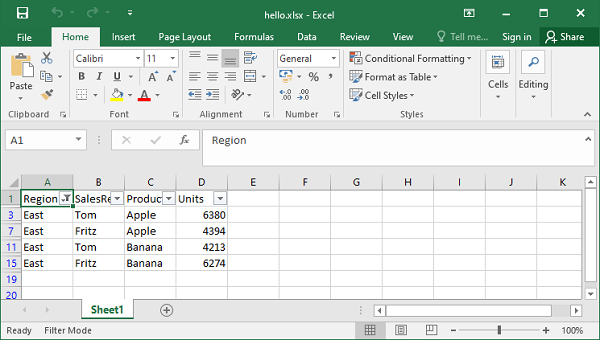
The column parameter can either be a zero indexed column number or a string column name. All the logical operators allowed in Python can be used in criteria (==, !=, <, >, <=, >=). Filter criteria can be defined on more than one columns and they can be combined by and or or operators. An example of criteria with logical operator can be as follows −
ws.filter_column('A', 'x > 2000')
ws.filter_column('A', 'x != 2000')
ws.filter_column('A', 'x > 2000 and x<5000')
Note that «x» in the criteria argument is just a formal place holder and can be any suitable string as it is ignored anyway internally.
ws.filter_column('A', 'price > 2000')
ws.filter_column('A', 'x != 2000')
ws.filter_column('A', 'marks > 60 and x<75')
XlsxWriter also allows the use of wild cards «*» and «?» in the filter criteria on columns containing string data.
ws.filter_column('A', name=K*') #starts with K
ws.filter_column('A', name=*K*') #contains K
ws.filter_column('A', name=?K*') # second character as K
ws.filter_column('A', name=*K??') #any two characters after K
Example
In the following example, first filter on column A requires region to be West and second filter’s criteria on column D is «units > 5000«. Rows not satisfying the condition «region = West» or «units > 5000» are hidden.
import xlsxwriter

wb = xlsxwriter.Workbook('hello.xlsx')
ws = wb.add_worksheet()

data = (
   ['Region',  'SalesRep', 'Product', 'Units'],
   ['East',    'Tom',      'Apple',    6380],
   ['West',    'Fred',     'Grape',    5619],
   ['North',   'Amy',      'Pear',     4565],
   ['South',   'Sal',      'Banana',   5323],
   ['East',    'Fritz',    'Apple',    4394],
   ['West',    'Sravan',   'Grape',    7195],
   ['North',   'Xi',       'Pear',     5231],
   ['South',   'Hector',   'Banana',   2427],
   ['East',    'Tom',      'Banana',   4213],
   ['West',    'Fred',     'Pear',     3239],
   ['North',   'Amy',      'Grape',    6520],
   ['South',   'Sal',      'Apple',    1310],
   ['East',    'Fritz',    'Banana',   6274],
   ['West',    'Sravan',   'Pear',     4894],
   ['North',   'Xi',       'Grape',    7580],
   ['South',   'Hector',   'Apple',    9814])

for row in range(len(data)):
   ws.write_row(row,0, data[row])

ws.autofilter(0, 0, 50, 3)

ws.filter_column('A', 'x == West')
ws.filter_column('D', 'x > 5000')

row = 1
for row_data in (data[1:]):
   region = row_data[0]
   volume = int(row_data[3])

   if region == 'West' or volume > 5000:
      pass
   else:
      ws.set_row(row, options={'hidden': True})

   ws.write_row(row, 0, row_data)
   row += 1

wb.close()
Output
In Excel, the filter icon can be seen on columns A and D headings. The filtered data is seen as below −
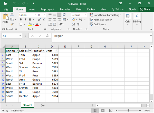
Applying a Column List Filter
The filter_column_list() method can be used to represent filters with multiple selected criteria in Excel 2007 style.
ws.filter_column_list(col,list)
The second argument is a list of values against which the data in a given column is matched. For example −
ws.filter_column_list('C', ['March', 'April', 'May'])
It results in filtering the data so that value in column C matches with any item in the list.
Example
In the following example, the filter_column_list() method is used to filter the rows with region equaling either East or West.
import xlsxwriter
wb = xlsxwriter.Workbook('hello.xlsx')
ws = wb.add_worksheet()
data = (
   ['Region', 'SalesRep', 'Product', 'Units'],
   ['East',   'Tom',      'Apple',    6380],
   ['West',   'Fred',     'Grape',    5619],
   ['North',  'Amy',      'Pear',     4565],
   ['South',  'Sal',      'Banana',   5323],
   ['East',   'Fritz',    'Apple',    4394],
   ['West',   'Sravan',   'Grape',    7195],
   ['North',  'Xi',       'Pear',     5231],
   ['South',  'Hector',   'Banana',   2427],
   ['East',   'Tom',      'Banana',   4213],
   ['West',   'Fred',     'Pear',     3239],
   ['North',  'Amy',      'Grape',    6520],
   ['South',  'Sal',      'Apple',    1310],
   ['East',   'Fritz',    'Banana',   6274],
   ['West',   'Sravan',   'Pear',     4894],
   ['North',  'Xi',       'Grape',    7580],
   ['South',  'Hector',   'Apple',    9814]
)
for row in range(len(data)):
   ws.write_row(row,0, data[row])

ws.autofilter(0, 0, 50, 3)

l1= ['East', 'West']
ws.filter_column_list('A', l1)

row = 1
for row_data in (data[1:]):
   region = row_data[0]

   if region not in l1:
      ws.set_row(row, options={'hidden': True})

   ws.write_row(row, 0, row_data)
   row += 1

wb.close()
Output
The Column A shows that the autofilter is applied. All the rows with Region as East or West are displayed and rest are hidden.
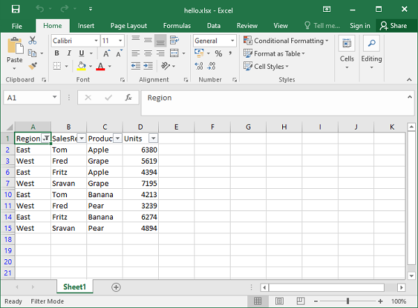
From the Excel software, click on the filter selector arrow in the Region heading and we should see that the filter on region equal to East or West is applied.
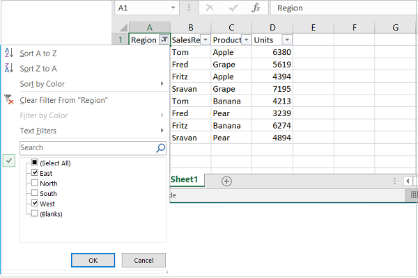
Python XlsxWriter — Fonts & Colors
Working with Fonts
To perform formatting of worksheet cell, we need to use Format object with the help of add_format() method and configure it with its properties or formatting methods.
f1 = workbook.add_format()
f1 = set_bold(True)
# or
f2 = wb.add_format({'bold':True})
This format object is then used as an argument to worksheet’s write() method.
ws.write('B1', 'Hello World', f1)
Example
To make the text in a cell bold, underline, italic or strike through, we can either use these properties or corresponding methods. In the following example, the text Hello World is written with set methods.
import xlsxwriter

wb = xlsxwriter.Workbook('hello.xlsx')
ws = wb.add_worksheet()

for row in range(4):
   ws.write(row,0, "Hello World")

f1=wb.add_format()
f2=wb.add_format()
f3=wb.add_format()
f4=wb.add_format()

f1.set_bold(True)
ws.write('B1', '=A1', f1)

f2.set_italic(True)
ws.write('B2', '=A2', f2)

f3.set_underline(True)
ws.write('B3', '=A3', f3)

f4.set_font_strikeout(True)
ws.write('B4', '=A4', f4)

wb.close()
Output
Here is the result −
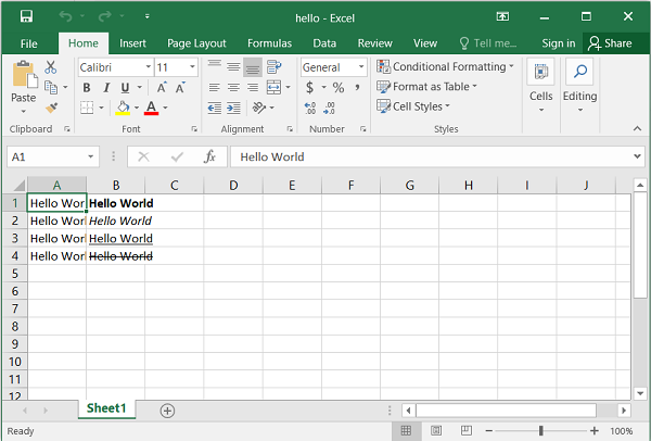
Example
On the other hand, we can use font_color, font_name and font_size properties to format the text as in the following example −
import xlsxwriter

wb = xlsxwriter.Workbook('hello.xlsx')
ws = wb.add_worksheet()

for row in range(4):
   ws.write(row,0, "Hello World")

f1=wb.add_format({'bold':True, 'font_color':'red'})
f2=wb.add_format({'italic':True,'font_name':'Arial'})
f3=wb.add_format({'font_size':20})
f4=wb.add_format({'font_color':'blue','font_size':14,'font_name':'Times New Roman'})

ws.write('B1', '=A1', f1)
ws.write('B2', '=A2', f2)
ws.write('B3', '=A3', f3)
ws.write('B4', '=A4', f4)

wb.close()
Output
The output of the above code can be verified by opening the worksheet with Excel −
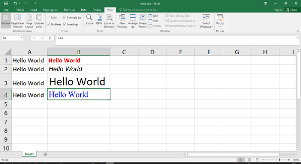
Text Alignment
XlsxWriter’s Format object can also be created with alignment methods/properties. The align property can have left, right, center and justify values.
Example
import xlsxwriter
wb = xlsxwriter.Workbook('hello.xlsx')
ws = wb.add_worksheet()
for row in range(4):
   ws.write(row,0, "Hello World")
ws.set_column('B:B', 30)

f1=wb.add_format({'align':'left'})
f2=wb.add_format({'align':'right'})
f3=wb.add_format({'align':'center'})
f4=wb.add_format({'align':'justify'})
ws.write('B1', '=A1', f1)
ws.write('B2', '=A2', f2)
ws.write('B3', '=A3', f3)
ws.write('B4', 'Hello World', f4)

wb.close()
Output
The following output shows the text «Hello World» with different alignments. Note that the width of B column is set to 30 by set_column() method of the worksheet object.
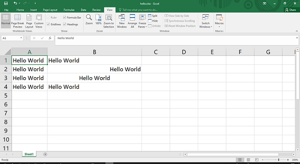
Example
Format object also has valign properties to control vertical placement of the cell.
import xlsxwriter

wb = xlsxwriter.Workbook('hello.xlsx')
ws = wb.add_worksheet()

for row in range(4):
   ws.write(row,0, "Hello World")

ws.set_column('B:B', 30)

for row in range(4):
   ws.set_row(row, 40)
f1=wb.add_format({'valign':'top'})
f2=wb.add_format({'valign':'bottom'})
f3=wb.add_format({'align':'vcenter'})
f4=wb.add_format({'align':'vjustify'})

ws.write('B1', '=A1', f1)
ws.write('B2', '=A2', f2)
ws.write('B3', '=A3', f3)
ws.write('B4', '=A4', f4)

wb.close()
Output
In the above code, the height of rows 1 to 4 is set to 40 with set_row() method.
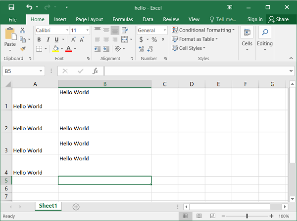
Cell Background and Foreground Colors
Two important properties of Format object are bg_color and fg_color to set the background and foreground color of a cell.
Example
import xlsxwriter

wb = xlsxwriter.Workbook('hello.xlsx')
ws = wb.add_worksheet()
ws.set_column('B:B', 30)

f1=wb.add_format({'bg_color':'red', 'font_size':20})
f2=wb.add_format({'bg_color':'#0000FF', 'font_size':20})

ws.write('B1', 'Hello World', f1)
ws.write('B2', 'HELLO WORLD', f2)
wb.close()
Output
The result of above code looks like this −
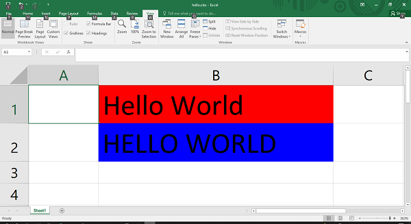
Python XlsxWriter — Number Formats
In Excel, different formatting options of numeric data are provided in the Number tab of Format Cells menu.
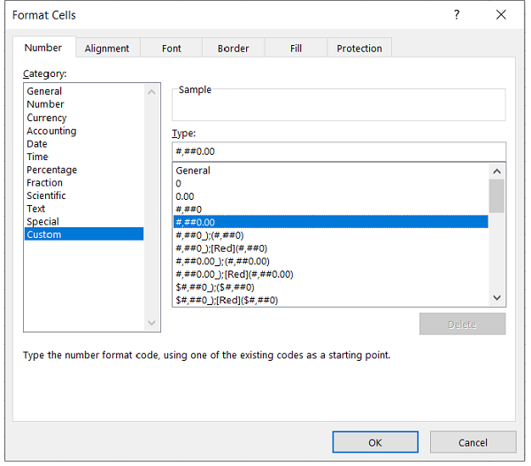
To control the formatting of numbers with XlsxWriter, we can use the set_num_format() method or define num_format property of add_format() method.
f1 = wb.add_format()
f1.set_num_format(FormatCode)
#or
f1 = wb.add_format('num_format': FormatCode)
Excel has a number of predefined number formats. They can be found under the custom category of Number tab as shown in the above figure. For example, the format code for number with two decimal points and comma separator is #,##0.00.
Example
In the following example, a number 1234.52 is formatted with different format codes.
import xlsxwriter

wb = xlsxwriter.Workbook('hello.xlsx')
ws = wb.add_worksheet()
ws.set_column('B:B', 30)

num=1234.52

num_formats = (
   '0.00',
   '#,##0.00',
   '0.00E+00',
   '##0.0E+0',
   '₹#,##0.00',
)
ws.write('A1', 'Formatted Number')
ws.write('B1', 'Format')

row = 1
for fmt in num_formats:
   format = wb.add_format({'num_format': fmt})
   ws.write_number(row, 0, num, format)
   ws.write_string(row, 1, fmt)
   row += 1
wb.close()
Output
The formatted number along with the format code used is shown in the following figure −
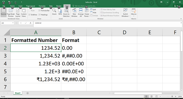
Python XlsxWriter — Border
This section describes how to apply and format the appearance of cell border as well as a border around text box.
Working with Cell Border
The properties in the add_format() method that control the appearance of cell border are as shown in the following table −
| Description | Property | method |
|---|---|---|
| Cell border | ‘border’ | set_border() |
| Bottom border | ‘bottom’ | set_bottom() |
| Top border | ‘top’ | set_top() |
| Left border | ‘left’ | set_left() |
| Right border | ‘right’ | set_right() |
| Border color | ‘border_color’ | set_border_color() |
| Bottom color | ‘bottom_color’ | set_bottom_color() |
| Top color | ‘top_color’ | set_top_color() |
| Left color | ‘left_color’ | set_left_color() |
| Right color | ‘right_color’ | set_right_color() |
Note that for each property of add_format() method, there is a corresponding format class method starting with the set_propertyname() method.
For example, to set a border around a cell, we can use border property in add_format() method as follows −
f1= wb.add_format({ 'border':2})
The same action can also be done by calling the set_border() method −
f1 = workbook.add_format()
f1.set_border(2)
Individual border elements can be configured by the properties or format methods as follows −
- set_bottom()
- set_top()
- set_left()
- set_right()
These border methods/properties have an integer value corresponding to the predefined styles as in the following table −
| Index | Name | Weight | Style |
|---|---|---|---|
| 0 | None | 0 | |
| 1 | Continuous | 1 | ———— |
| 2 | Continuous | 2 | ———— |
| 3 | Dash | 1 | — — — — — — |
| 4 | Dot | 1 | . . . . . . |
| 5 | Continuous | 3 | ———— |
| 6 | Double | 3 | =========== |
| 7 | Continuous | 0 | ———— |
| 8 | Dash | 2 | — — — — — — |
| 9 | Dash Dot | 1 | — . — . — . |
| 10 | Dash Dot | 2 | — . — . — . |
| 11 | Dash Dot Dot | 1 | — . . — . . |
| 12 | Dash Dot Dot | 2 | — . . — . . |
| 13 | SlantDash Dot | 2 | / — . / — . |
Example
Following code shows how the border property is used. Here, each row is having a border style 2 corresponding to continuous bold.
import xlsxwriter

wb = xlsxwriter.Workbook('hello.xlsx')
ws = wb.add_worksheet()

f1=wb.add_format({'bold':True, 'border':2, 'border_color':'red'})
f2=wb.add_format({'border':2, 'border_color':'red'})

headings = ['Month', 'Product A', 'Product B']

data = [
   ['Jan', 'Feb', 'Mar', 'Apr', 'May', 'June'],
   [10, 40, 50, 20, 10, 50],
   [30, 60, 70, 50, 40, 30],
]

ws.write_row('A1', headings, f1)
ws.write_column('A2', data[0], f2)
ws.write_column('B2', data[1],f2)
ws.write_column('C2', data[2],f2)

wb.close()
Output
The worksheet shows a bold border around the cells.
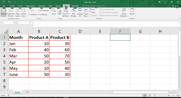
Working with Textbox Border
The border property is also available for the text box object. The text box also has a line property which is similar to border, so that they can be used interchangeably. The border itself can further be formatted by none, color, width and dash_type parameters.
Line or border set to none means that the text box will not have any border. The dash_type parameter can be any of the following values −
- solid
- round_dot
- square_dot
- dash
- dash_dot
- long_dash
- long_dash_dot
- long_dash_dot_dot
Example
Here is a program that displays two text boxes, one with a solid border, red in color; and the second box has dash_dot type border in blue color.
import xlsxwriter

wb = xlsxwriter.Workbook('hello.xlsx')
ws = wb.add_worksheet()

ws.insert_textbox('B2', 'Welcome to Tutorialspoint',
{'border': {'color': '#FF9900'}})

ws.insert_textbox('B10', 'Welcome to Tutorialspoint', {
   'line':
   {'color': 'blue', 'dash_type': 'dash_dot'}
})
wb.close()
Output
The output worksheet shows the textbox borders.
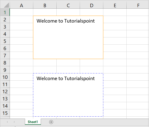
Python XlsxWriter — Hyperlinks
A hyperlink is a string, which when clicked, takes the user to some other location, such as a URL, another worksheet in the same workbook or another workbook on the computer. Worksheet class provides write_url() method for the purpose. Hyperlinks can also be placed inside a textbox with the use of url property.
First, let us learn about write_url() method. In addition to the Cell location, it needs the URL string to be directed to.
import xlsxwriter

workbook = xlsxwriter.Workbook('hello.xlsx')
worksheet = workbook.add_worksheet()
worksheet.write_url('A1', 'https://www.tutorialspoint.com/index.htm')

workbook.close()
This method has a few optional parameters. One is a Format object to configure the font, color properties of the URL to be displayed. We can also specify a tool tip string and a display text foe the URL. When the text is not given, the URL itself appears in the cell.
Example
Different types of URLs supported are http://, https://, ftp:// and mailto:. In the example below, we use these URLs.
import xlsxwriter

workbook = xlsxwriter.Workbook('hello.xlsx')
worksheet = workbook.add_worksheet()

worksheet.write_url('A1', 'https://www.tutorialspoint.com/index.htm')
worksheet.write_url('A3', 'http://localhost:8080')
worksheet.write_url('A5', 'ftp://www.python.org')
worksheet.write_url('A7', 'mailto:dummy@abc.com')

workbook.close()
Output
Run the above code and open the hello.xlsx file using Excel.
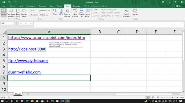
Example
We can also insert hyperlink to either another workskeet in the same workbook, or another workbook. This is done by prefixing with internal: or external: the local URIs.
import xlsxwriter

workbook = xlsxwriter.Workbook('hello.xlsx')
worksheet = workbook.add_worksheet()

worksheet.write_url('A1', 'internal:Sheet2!A1', string="Link to sheet2", tip="Click here")
worksheet.write_url('A4', "external:c:/test/testlink.xlsx", string="Link to other workbook")

workbook.close()
Output
Note that the string and tip parameters are given as an alternative text to the link and tool tip. The output of the above program is as given below −
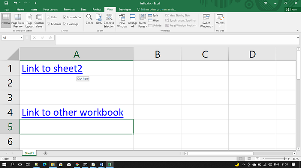
Python XlsxWriter — Conditional Formatting
Excel uses conditional formatting to change the appearance of cells in a range based on user defined criteria. From the conditional formatting menu, it is possible to define criteria involving various types of values.
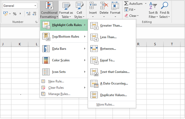
In the worksheet shown below, the column A has different numbers. Numbers less than 50 are shown in red font color and grey background color.
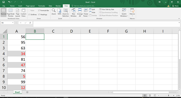
This is achieved by defining a conditional formatting rule below −
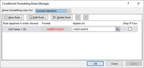
The conditional_format() method
In XlsxWriter, there as a conditional_format() method defined in the Worksheet class. To achieve the above shown result, the conditional_format() method is called as in the following code −
import xlsxwriter

wb = xlsxwriter.Workbook('hello.xlsx')
ws = wb.add_worksheet()

data=[56,95,63,34,81,47,74,5,99,12]
row=0

for num in data:
   ws.write(row,0,num)
   row+=1
f1 = wb.add_format({'bg_color': '#D9D9D9', 'font_color': 'red'})
ws.conditional_format(
   'A1:A10',{
      'type':'cell', 'criteria':'<', 'value':50, 'format':f1
   }
)
wb.close()
Parameters
The conditional_format() method’s first argument is the cell range, and the second argument is a dictionary of conditional formatting options.
The options dictionary configures the conditional formatting rules with the following parameters −
The type option is a required parameter. Its value is either cell, date, text, formula, etc. Each parameter has sub-parameters such as criteria, value, format, etc.
-
Type is the most common conditional formatting type. It is used when a format is applied to a cell based on a simple criterion.
-
Criteria parameter sets the condition by which the cell data will be evaluated. All the logical operator in addition to between and not between operators are the possible values of criteria parameter.
-
Value parameter is the operand of the criteria that forms the rule.
-
Format parameter is the Format object (returned by the add_format() method). This defines the formatting features such as font, color, etc. to be applied to cells satisfying the criteria.
The date type is similar the cell type and uses the same criteria and values. However, the value parameter should be given as a datetime object.
The text type specifies Excel’s «Specific Text» style conditional format. It is used to do simple string matching using the criteria and value parameters.
Example
When formula type is used, the conditional formatting depends on a user defined formula.
import xlsxwriter

wb = xlsxwriter.Workbook('hello.xlsx')
ws = wb.add_worksheet()

data = [
   ['Anil', 45, 55, 50], ['Ravi', 60, 70, 80],
   ['Kiran', 65, 75, 85], ['Karishma', 55, 65, 45]
]
for row in range(len(data)):
   ws.write_row(row,0, data[row])

f1 = wb.add_format({'font_color': 'blue', 'bold':True})

ws.conditional_format(
   'A1:D4',
   {
      'type':'formula', 'criteria':'=AVERAGE($B1:$D1)>60', 'value':50, 'format':f1
   })
wb.close()
Output
Open the resultant workbook using MS Excel. We can see the rows satisfying the above condition displayed in blue color according to the format object. The conditional format rule manager also shows the criteria that we have set in the above code.
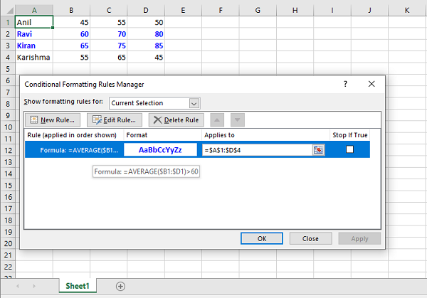
Python XlsxWriter — Adding Charts
One of the most important features of Excel is its ability to convert data into chart. A chart is a visual representation of data. Different types of charts can be generated from the Chart menu.
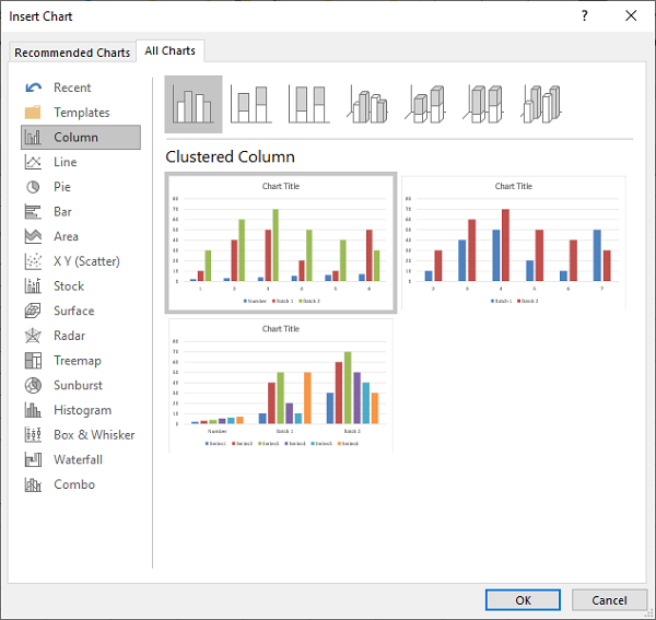
To generate charts programmatically, XlsxWriter library has a Chart class. Its object is obtained by calling add_chart() method of the Workbook class. It is then associated with the data ranges in the worksheet with the help of add_series() method. The chart object is then inserted in the worksheet using its insert_chart() method.
Example
Given below is the code for displaying a simple column chart.
import xlsxwriter
wb = xlsxwriter.Workbook('hello.xlsx')
worksheet = wb.add_worksheet()
chart = wb.add_chart({'type': 'column'})

data = [
   [10, 20, 30,  40,  50],
   [20, 40, 60,  80, 100],
   [30, 60, 90, 120, 150],
]
worksheet.write_column('A1', data[0])
worksheet.write_column('B1', data[1])
worksheet.write_column('C1', data[2])

chart.add_series({'values': '=Sheet1!$A$1:$A$5'})
chart.add_series({'values': '=Sheet1!$B$1:$B$5'})
chart.add_series({'values': '=Sheet1!$C$1:$C$5'})

worksheet.insert_chart('B7', chart)

wb.close()
Output
The generated chart is embedded in the worksheet and appears as follows −
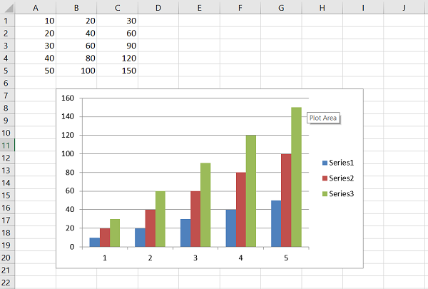
The add_series() method has following additional parameters −
-
Values − This is the most important property mandatory option. It links the chart with the worksheet data that it displays.
-
Categories − This sets the chart category labels. If not given, the chart will just assume a sequential series from 1…n.
-
Name − Set the name for the series. The name is displayed in the formula bar.
-
Line − Set the properties of the series line type such as color and width.
-
Border − Set the border properties of the series such as color and style.
-
Fill − Set the solid fill properties of the series such as color.
-
Pattern − Set the pattern fill properties of the series.
-
Gradient − Set the gradient fill properties of the series.
-
data_labels − Set data labels for the series.
-
Points − Set properties for individual points in a series.
In the following examples, while adding the data series, the value and categories properties are defined. The data for the example is −
# Add the worksheet data that the charts will refer to.
headings = ['Name', 'Phy', 'Maths']
data = [
   ["Jay",   30, 60],
   ["Mohan", 40, 50],
   ["Veeru", 60, 70],
]
After creating the chart object, the first data series corresponds to the column with phy as the value of name property. Names of the students in the first column are used as categories
chart1.add_series({
   'name': '=Sheet1!$B$1',
   'categories': '=Sheet1!$A$2:$A$4',
   'values': '=Sheet1!$B$2:$B$4',
})
The second data series too refers to names in column A as categories and column C with heading as Maths as the values property.
chart1.add_series({
   'name': ['Sheet1', 0, 2],
   'categories': ['Sheet1', 1, 0, 3, 0],
   'values': ['Sheet1', 1, 2, 3, 2],
})
Example
Here is the complete example code −
import xlsxwriter
wb = xlsxwriter.Workbook('hello.xlsx')
worksheet = wb.add_worksheet()
chart1 = wb.add_chart({'type': 'column'})

# Add the worksheet data that the charts will refer to.
headings = ['Name', 'Phy', 'Maths']
data = [
   ["Jay",   30, 60],
   ["Mohan", 40, 50],
   ["Veeru", 60, 70],
]

worksheet.write_row(0,0, headings)
worksheet.write_row(1,0, data[0])
worksheet.write_row(2,0, data[1])
worksheet.write_row(3,0, data[2])

chart1.add_series({
   'name': '=Sheet1!$B$1',
   'categories': '=Sheet1!$A$2:$A$4',
   'values': '=Sheet1!$B$2:$B$4',
})

chart1.add_series({
   'name': ['Sheet1', 0, 2],
   'categories': ['Sheet1', 1, 0, 3, 0],
   'values': ['Sheet1', 1, 2, 3, 2],
})

worksheet.insert_chart('B7', chart1)

wb.close()
Output
The worksheet and the chart based on it appears as follows −
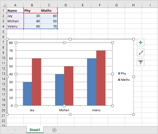
The add_series() method also has data_labels property. If set to True, values of the plotted data points are displayed on top of each column.
Example
Here is the complete code example for add_series() method −
import xlsxwriter
wb = xlsxwriter.Workbook('hello.xlsx')
worksheet = wb.add_worksheet()
chart1 = wb.add_chart({'type': 'column'})

# Add the worksheet data that the charts will refer to.
headings = ['Name', 'Phy', 'Maths']
data = [
   ["Jay",   30, 60],
   ["Mohan", 40, 50],
   ["Veeru", 60, 70],
]

worksheet.write_row(0,0, headings)
worksheet.write_row(1,0, data[0])
worksheet.write_row(2,0, data[1])
worksheet.write_row(3,0, data[2])

chart1.add_series({
   'name': '=Sheet1!$B$1',
   'categories': '=Sheet1!$A$2:$A$4',
   'values': '=Sheet1!$B$2:$B$4',
   'data_labels': {'value':True},
})
chart1.add_series({
   'name': ['Sheet1', 0, 2],
   'categories': ['Sheet1', 1, 0, 3, 0],
   'values': ['Sheet1', 1, 2, 3, 2],
   'data_labels': {'value':True},
})
worksheet.insert_chart('B7', chart1)

wb.close()
Output
Execute the code and open Hello.xlsx. The column chart now shows the data labels.
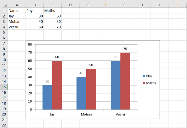
The data labels can be displayed for all types of charts. Position parameter of data label can be set to top, bottom, left or right.
XlsxWriter supports the following types of charts −
-
Area − Creates an Area (filled line) style chart.
-
Bar − Creates a Bar style (transposed histogram) chart.
-
Column − Creates a column style (histogram) chart.
-
Line − Creates a Line style chart.
-
Pie − Creates a Pie style chart.
-
Doughnut − Creates a Doughnut style chart.
-
Scatter − Creates a Scatter style chart.
-
Stock − Creates a Stock style chart.
-
Radar − Creates a Radar style chart.
Many of the chart types also have subtypes. For example, column, bar, area and line charts have sub types as stacked and percent_stacked. The type and subtype parameters can be given in the add_chart() method.
workbook.add_chart({'type': column, 'subtype': 'stacked'})
The chart is embedded in the worksheet with its insert_chart() method that takes following parameters −
worksheet.insert_chart(location, chartObj, options)
The options parameter is a dictionary that configures the position and scale of chart. The option properties and their default values are −
{
   'x_offset':        0,
   'y_offset':        0,
   'x_scale':         1,
   'y_scale':         1,
   'object_position': 1,
   'description':     None,
   'decorative':      False,
}
The x_offset and y_offset values are in pixels, whereas x_scale and y_scale values are used to scale the chart horizontally / vertically. The description field can be used to specify a description or «alt text» string for the chart.
The decorative parameter is used to mark the chart as decorative, and thus uninformative, for automated screen readers. It has to be set to True/False. Finally, the object_position parameter controls the object positioning of the chart. It allows the following values −
-
1 − Move and size with cells (the default).
-
2 − Move but don’t size with cells.
-
3 − Don’t move or size with cells.
Python XlsxWriter — Chart Formatting
The default appearance of chart can be customized to make it more appealing, explanatory and user friendly. With XlsxWriter, we can do following enhancements to a Chart object −
-
Set and format chart title
-
Set the X and Y axis titles and other parameters
-
Configure the chart legends
-
Chat layout options
-
Setting borders and patterns
Title
You can set and configure the main title of a chart object by calling its set_title() method. Various parameters that can be are as follows −
-
Name − Set the name (title) for the chart to be displayed above the chart. The name property is optional. The default is to have no chart title.
-
name_font − Set the font properties for the chart title.
-
Overlay − Allow the title to be overlaid on the chart.
-
Layout − Set the (x, y) position of the title in chart relative units.
-
None − Excel adds an automatic chart title. The none option turns this default title off. It also turns off all other set_title() options.
X and Y axis
The two methods set_x_axis() and set_y_axis() are used to axis titles, the name_font to be used for the title text, the num_font to be used for numbers displayed on the X and Y axis.
-
name − Set the title or caption for the axis.
-
name_font − Set the font properties for the axis title.
-
num_font − Set the font properties for the axis numbers.
-
num_format − Set the number format for the axis.
-
major_gridlines − Configure the major gridlines for the axis.
-
display_units − Set the display units for the axis.
In the previous example, where the data of marklist has been shown in the form of a column chart, we set up the chart formatting options such as the chart title and X as well as Y axis captions and their other display properties as follows −
chart1.set_x_axis(
   {'name': 'Students', 'name_font':{'name':'Arial', 'size':16, 'bold':True},})
chart1.set_y_axis(
   {
      'name': 'Marks', 'name_font':
      {'name':'Arial', 'size':16, 'bold':True}, 'num_font':{'name':'Arial', 'italic':True}
   }
)
Example
Add the above snippet in the complete code. It now looks as given below −
import xlsxwriter

wb = xlsxwriter.Workbook('hello.xlsx')
worksheet = wb.add_worksheet()
chart1 = wb.add_chart({'type': 'column'})

# Add the worksheet data that the charts will refer to.
headings = ['Name', 'Phy', 'Maths']

data = [
   ["Jay", 30, 60],
   ["Mohan", 40, 50],
   ["Veeru", 60, 70],
]

worksheet.write_row(0,0, headings)
worksheet.write_row(1,0, data[0])
worksheet.write_row(2,0, data[1])
worksheet.write_row(3,0, data[2])

chart1.add_series({
   'name': '=Sheet1!$B$1',
   'categories': '=Sheet1!$A$2:$A$4',
   'values': '=Sheet1!$B$2:$B$4',
})

chart1.add_series({
   'name': ['Sheet1', 0, 2],
   'categories': ['Sheet1', 1, 0, 3, 0],
   'values': ['Sheet1', 1, 2, 3, 2],
})
chart1.set_title ({'name': 'Marklist',
   'name_font': {'name':'Times New Roman', 'size':24}
})
chart1.set_x_axis({'name': 'Students',
   'name_font': {'name':'Arial', 'size':16, 'bold':True},
})
chart1.set_y_axis({'name': 'Marks',
   'name_font':{'name':'Arial', 'size':16, 'bold':True},
   'num_font':{'name':'Arial', 'italic':True}
})
worksheet.insert_chart('B7', chart1)

wb.close()
Output
The chart shows the title and axes captions as follows −
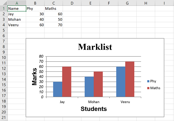
Python XlsxWriter — Chart Legends
Depending upon the type of chart, the data is visually represented in the form of columns, bars, lines, arcs, etc. in different colors or patterns. The chart legend makes it easy to quickly understand which color/pattern corresponds to which data series.
Working with Chart Legends
To set the legend and configure its properties such as position and font, XlsxWriter has set_legend() method. The properties are −
-
None − In Excel chart legends are on by default. The none=True option turns off the chart legend.
-
Position − Set the position of the chart legend. It can be set to top, bottom, left, right, none.
-
Font − Set the font properties (like name, size, bold, italic etc.) of the chart legend.
-
Border − Set the border properties of the legend such as color and style.
-
Fill − Set the solid fill properties of the legend such as color.
-
Pattern − Set the pattern fill properties of the legend.
-
Gradient − Set the gradient fill properties of the legend.
Some of the legend properties are set for the chart as below −
chart1.set_legend(
   {'position':'bottom', 'font': {'name':'calibri','size': 9, 'bold': True}}
)
Example
Here is the complete code to display legends as per the above characteristics −
import xlsxwriter

wb = xlsxwriter.Workbook('hello.xlsx')
worksheet = wb.add_worksheet()
chart1 = wb.add_chart({'type': 'column'})

# Add the worksheet data that the charts will refer to.
headings = ['Name', 'Phy', 'Maths']
data = [
   ["Jay", 30, 60],
   ["Mohan", 40, 50],
   ["Veeru", 60, 70],
]

worksheet.write_row(0,0, headings)
worksheet.write_row(1,0, data[0])
worksheet.write_row(2,0, data[1])
worksheet.write_row(3,0, data[2])
chart1.add_series({
   'name': '=Sheet1!$B$1',
   'categories': '=Sheet1!$A$2:$A$4',
   'values': '=Sheet1!$B$2:$B$4',
})
chart1.add_series({
   'name': ['Sheet1', 0, 2],
   'categories': ['Sheet1', 1, 0, 3, 0],
   'values': ['Sheet1', 1, 2, 3, 2],
})
chart1.set_title ({'name': 'Marklist', 'name_font':
   {'name':'Times New Roman', 'size':24}})

chart1.set_x_axis({'name': 'Students', 'name_font':
   {'name':'Arial', 'size':16, 'bold':True},})

chart1.set_y_axis({'name': 'Marks','name_font':
   {'name':'Arial', 'size':16, 'bold':True},
   'num_font':{'name':'Arial', 'italic':True}})

chart1.set_legend({'position':'bottom', 'font':
   {'name':'calibri','size': 9, 'bold': True}})

worksheet.insert_chart('B7', chart1)

wb.close()
Output
The chart shows the legend below the caption of the X axis.
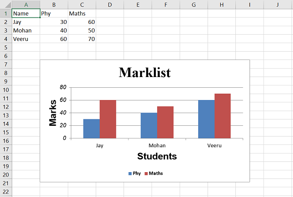
In the chart, the columns corresponding to physics and maths are shown in different colors. The small colored box symbols to the right of the chart are the legends that show which color corresponds to physics or maths.
Python XlsxWriter — Bar Chart
The bar chart is similar to a column chart, except for the fact that the data is represented in proportionate horizontal bars instead of vertical columns. To produce a bar chart, the type argument of add_chart() method must be set to ‘bar’.
chart1 = workbook.add_chart({'type': 'bar'})
The bar chart appears as follows −
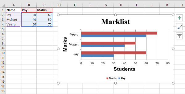
There are two subtypes of bar chart, namely stacked and percent_stacked. In the stacked chart, the bars of different colors for a certain category are placed one after the other. In a percent_stacked chart, the length of each bar shows its percentage in the total value in each category.
chart1 = workbook.add_chart({
   'type': 'bar',
   'subtype': 'percent_stacked'
})
Example
Program to generate percent stacked bar chart is given below −
import xlsxwriter

wb = xlsxwriter.Workbook('hello.xlsx')
worksheet = wb.add_worksheet()
chart1 = wb.add_chart({'type': 'bar', 'subtype': 'percent_stacked'})

# Add the worksheet data that the charts will refer to.
headings = ['Name', 'Phy', 'Maths']
data = [
   ["Jay", 30, 60],
   ["Mohan", 40, 50],
   ["Veeru", 60, 70],
]

worksheet.write_row(0,0, headings)
worksheet.write_row(1,0, data[0])
worksheet.write_row(2,0, data[1])
worksheet.write_row(3,0, data[2])

chart1.add_series({
   'name': '=Sheet1!$B$1',
   'categories': '=Sheet1!$A$2:$A$4',
   'values': '=Sheet1!$B$2:$B$4',
})

chart1.add_series({
   'name': ['Sheet1', 0, 2],
   'categories': ['Sheet1', 1, 0, 3, 0],
   'values': ['Sheet1', 1, 2, 3, 2],
})
chart1.set_title ({'name': 'Marklist', 'name_font':
   {'name':'Times New Roman', 'size':24}})

chart1.set_x_axis({'name': 'Students', 'name_font':
   {'name':'Arial', 'size':16, 'bold':True}, })

chart1.set_y_axis({'name': 'Marks','name_font':
   {'name':'Arial', 'size':16, 'bold':True},
   'num_font':{'name':'Arial', 'italic':True}})

chart1.set_legend({'position':'bottom', 'font':
   {'name':'calibri','size': 9, 'bold': True}})

worksheet.insert_chart('B7', chart1)

wb.close()
Output
The output file will look like the one given below −
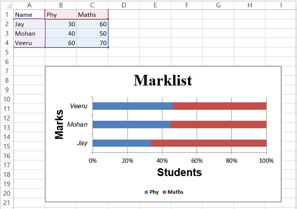
Python XlsxWriter — Line Chart
A line shows a series of data points connected with a line along the X-axis. It is an independent axis because the values on the X-axis do not depend on the vertical Y-axis.
The Y-axis is a dependent axis because its values depend on the X-axis and the result is the line that progress horizontally.
Working with XlsxWriter Line Chart
To generate the line chart programmatically using XlsxWriter, we use add_series(). The type of chart object is defined as ‘line‘.
Example
In the following example, we shall plot line chart showing the sales figures of two products over six months. Two data series corresponding to sales figures of Product A and Product B are added to the chart with add_series() method.
import xlsxwriter

wb = xlsxwriter.Workbook('hello.xlsx')
worksheet = wb.add_worksheet()
headings = ['Month', 'Product A', 'Product B']

data = [
   ['Jan', 'Feb', 'Mar', 'Apr', 'May', 'June'],
   [10, 40, 50, 20, 10, 50],
   [30, 60, 70, 50, 40, 30],
]

bold=wb.add_format({'bold':True})
worksheet.write_row('A1', headings, bold)
worksheet.write_column('A2', data[0])
worksheet.write_column('B2', data[1])
worksheet.write_column('C2', data[2])

chart1 = wb.add_chart({'type': 'line'})

chart1.add_series({
   'name': '=Sheet1!$B$1',
   'categories': '=Sheet1!$A$2:$A$7',
   'values': '=Sheet1!$B$2:$B$7',
})
chart1.add_series({
   'name': ['Sheet1', 0, 2],
   'categories': ['Sheet1', 1, 0, 6, 0],
   'values': ['Sheet1', 1, 2, 6, 2],
})
chart1.set_title ({'name': 'Sales analysis'})
chart1.set_x_axis({'name': 'Months'})
chart1.set_y_axis({'name': 'Units'})

worksheet.insert_chart('D2', chart1)

wb.close()
Output
After executing the above program, here is how XlsxWriter generates the Line chart −
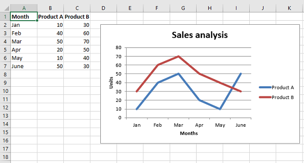
Along with data_labels, the add_series() method also has a marker property. This is especially useful in a line chart. The data points are indicated by marker symbols such as a circle, triangle, square, diamond etc. Let us assign circle and square symbols to the two data series in this chart.
chart1.add_series({
   'name': '=Sheet1!$B$1',
   'categories': '=Sheet1!$A$2:$A$7',
   'values': '=Sheet1!$B$2:$B$7',
   'data_labels': {'value': True},
   'marker': {'type': 'circle'},
})
chart1.add_series({
   'name': ['Sheet1', 0, 2],
   'categories': ['Sheet1', 1, 0, 6, 0],
   'values': ['Sheet1', 1, 2, 6, 2],
   'data_labels': {'value': True},
   'marker': {'type': 'square'},})
The data labels and markers are added to the line chart.
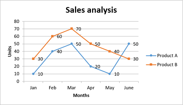
Line chart also supports stacked and percent_stacked subtypes.
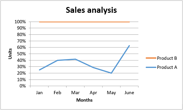
Python XlsxWriter — Pie Chart
A pie chart is a representation of a single data series into a circle, which is divided into slices corresponding to each data item in the series. In a pie chart, the arc length of each slice is proportional to the quantity it represents. In the following worksheet, quarterly sales figures of a product are displayed in the form of a pie chart.
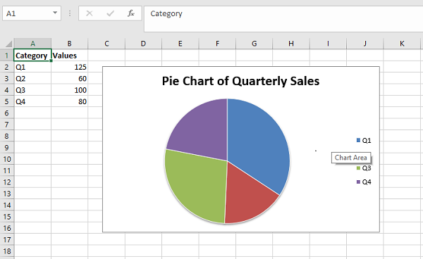
Working with XlsxWriter Pie Chart
To generate the above chart programmatically using XlsxWriter, we first write the following data in the worksheet.
headings = ['Category', 'Values']
data = [
   ['Q1', 'Q2', 'Q3', 'Q4'],
   [125, 60, 100, 80],
]
worksheet.write_row('A1', headings, bold)
worksheet.write_column('A2', data[0])
worksheet.write_column('B2', data[1])
A Chart object with type=pie is declared and the cell range B1:D1 is used as value parameter for add_series() method and the quarters (Q1, Q2, Q3 and Q4) in column A are the categories.
chart1.add_series({
   'name': 'Quarterly sales data',
   'categories': ['Sheet1', 1, 0, 4, 0],
   'values': ['Sheet1', 1, 1, 4, 1],
})
chart1.set_title({'name': 'Pie Chart of Quarterly Sales'})
In the pie chart, we can use data_labels property to represent the percent value of each pie by setting percentage=True.
Example
The complete program for pie chart generation is as follows −
import xlsxwriter

wb = xlsxwriter.Workbook('hello.xlsx')
worksheet = wb.add_worksheet()

headings = ['Category', 'Values']
data = [
   ['Q1', 'Q2', 'Q3', 'Q4'],
   [125, 60, 100, 80],
]
bold=wb.add_format({'bold':True})
worksheet.write_row('A1', headings, bold)
worksheet.write_column('A2', data[0])
worksheet.write_column('B2', data[1])

chart1 = wb.add_chart({'type': 'pie'})
chart1.add_series({
   'name': 'Quarterly sales data',
   'categories': ['Sheet1', 1, 0, 4, 0],
   'values': ['Sheet1', 1, 1, 4, 1],
   'data_labels': {'percentage':True},
})
chart1.set_title({'name': 'Pie Chart of Quarterly Sales'})

worksheet.insert_chart('D2', chart1)

wb.close()
Output
Have a look at the pie chart that the above program produces.
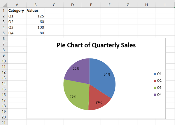
Doughnut Chart
The doughnut chart is a variant of the pie chart, with a hole in its center, and it displays categories as arcs rather than slices. Both make part-to-whole relationships easy to grasp at a glance. Just change the chart type to doughnut.
chart1 = workbook.add_chart({'type': 'doughnut'})
The doughnut chart of the data in above example appears as below −
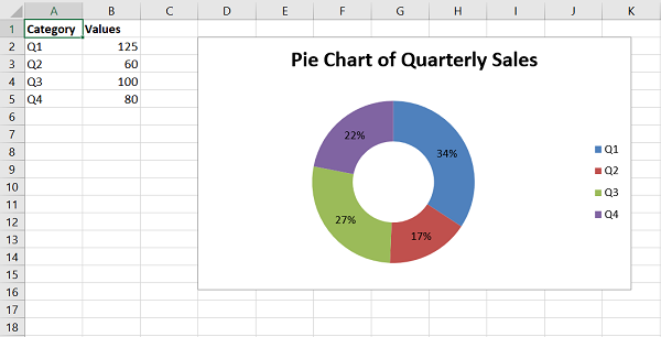
Python XlsxWriter — Sparklines
A sparkline is a small chart, that doesn’t have axes or coordinates. It gives a representation of variation of a certain parameter. Normal charts are bigger in size, with a lot of explanatory features such as title, legend, data labels etc. and are set off from the accompanying text. Sparkline on the other hand is small in size and can be embedded inside the text, or a worksheet cell that has its context.
Feature of Sparkline was introduced by Edward Tufte in 1983. Microsoft introduced sparklines in Excel 2010. We can find sparkline option in the insert ribbon of Excel software.
Sparklines are of three types −
-
line − Similar to line chart
-
column − Similar to column chart
-
win_loss − Whether each value is positive (win) or negative (loss).
Working with XlsxWriter Sparklines
XlsxWriter module has add_sparkline() method. It basically needs the cell location of the sparkline and the data range to be represented as a sparkline. Optionally, other parameters such as type, style, etc. are provided in the form of dictionary object. By default, the type is line.
Example
Following program represents same list of numbers in line and column sparklines.
import xlsxwriter

wb = xlsxwriter.Workbook('hello.xlsx')
ws = wb.add_worksheet()

data=[12,23,9,17,31,3,7,21,10,15]

ws.write_row('A1', data)
ws.set_column('K:K', 40)
ws.set_row(0, 30)
ws.add_sparkline('K1', {'range':'Sheet1!A1:J1'})

ws.write_row('A5', data)
ws.set_column('K:K', 40)
ws.set_row(4, 30)
ws.add_sparkline('K5', {'range':'Sheet1!A5:J5', 'type':'column'})

wb.close()
Output
In cell K, the sparklines are added.
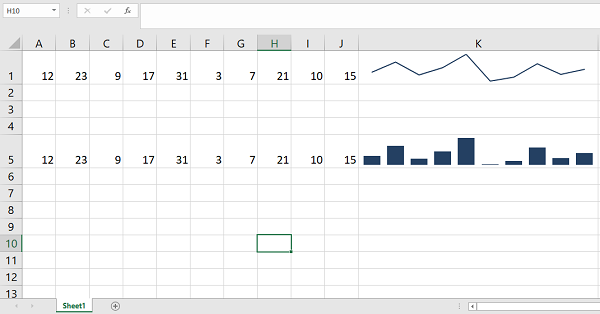
The properties are −
-
range − is the mandatory parameter. It specifies the cell data range that the sparkline will plot.
-
type − specifies the type of sparkline. There are 3 available sparkline types are line, column and win_loss.
-
markers − Turn on the markers for line style sparklines
-
style − The sparkline styles defined in MS Excel. There are 36 style types.
-
negative_points − If set to True, the negative points in a sparkline are highlighted.
Example
The following program produces a line sparkline with markers and a win_loss sparkline having negative points highlighted.
import xlsxwriter

wb = xlsxwriter.Workbook('hello.xlsx')
ws = wb.add_worksheet()

data=[12,23,9,17,31,3,7,21,10,15]
ws.write_row('A1', data)
ws.set_column('K:K', 40)
ws.set_row(0, 30)

data=[1,1,-1,-1,-1,1,1,1,-1,-1]
ws.write_row('A5', data)
ws.set_column('K:K', 40)
ws.set_row(4, 30)
ws.add_sparkline('K1', {'range':'Sheet1!A1:J1', 'markers':True})
ws.add_sparkline('K5', {'range':'Sheet1!A5:J5', 'type':'win_loss',
'negative_points':True})

wb.close()
Output
Line Sparkline in K1 has markers. The sparkline in K5 shows negative points highlighting.
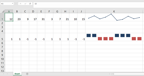
Example – Style Types
Following code displays a series of numbers in column sparkline. Ten different style types are used here.
import xlsxwriter

wb = xlsxwriter.Workbook('hello.xlsx')
ws = wb.add_worksheet()

data=[12,23,9,17,31,3,7,21,10,15]
ws.write_row('C3', data)
ws.set_column('B:B',40)

for i in range(1,11):
   ws.write(i+4,0, 'style {}'.format(i))
   ws.add_sparkline(i+4,1,
   {'range':'Sheet1!$C$3:$L$3',
   'type':'column',
   'style':i})

wb.close()
Output
It will produce the following output −
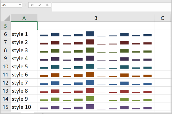
Python XlsxWriter — Data Validation
Data validation feature in Excel allows you to control what a user can enter into a cell. You can use it to ensure that the value in a cell is a number/date within a specified range, text with required length, or to present a dropdown menu to choose the value from.
The data validation tools are available in the Data menu. The first tab allows you to set a validation criterion. Following figure shows that criteria requires the cell should contain an integer between 1 to 25 −
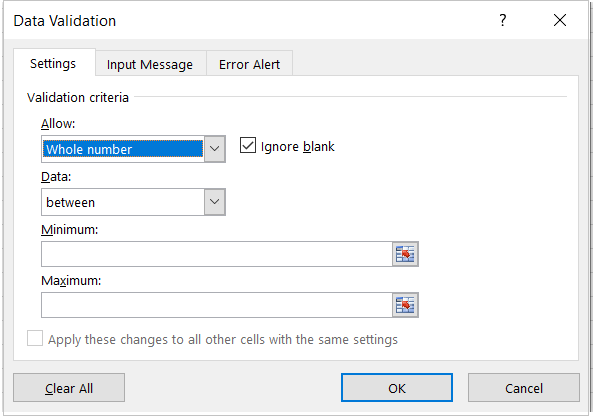
In the second tab, set the message to be flashed when user’s cursor is on the desired cell, which in this case is ‘Enter any integer between 1 to 25’. You can also set the message title; in this case it is Age.
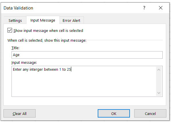
The third tab allows asks you to define any error message you would like to flash if the validation criteria fails.
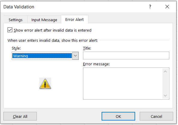
When the user places the cursor in I10 (for which the validation is set), you can see the input message.
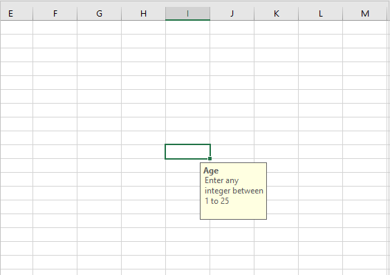
When the entered number is not in the range, the error message will flash.
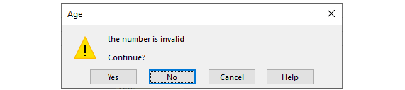
Working with XlsxWriter Data Validation
You can set the validation criteria, input and error message programmatically with data_validation() method.
worksheet.data_validation(
   'I10',
   {
      'validate': 'integer','criteria': 'between',
      'minimum': 1,'maximum': 25,
      'input_title': 'Enter an integer:',
      'input_message': 'between 1 and 25',
      'error_title': 'Input value is not valid!',
      'error_message': 'It  should be an integer between 1 and 25'
   }
)
The data_validation() method accepts options parameter as a dictionary with following parameters −
-
validate − It is used to set the type of data that you wish to validate. Allowed values are integer, decimal, list, date, time, length etc.
-
criteria − It is used to set the criteria for validation. It can be set to any logical operator including between/ not between, ==, !=, <, >, <=, >=, etc.
-
value − Sets the limiting value to which the criteria is applied. It is always required. When using the list validation, it is given as a Comma Separated Variable string.
-
input_title − Used to set the title of the input message when the cursor is placed in the target cell.
-
input_message − The message to be displayed when a cell is entered.
-
error_title − The title of the error message to be displayed when validation criteria is not met.
-
error_message − Sets the error message. The default error message is «The value you entered is not valid. A user has restricted values that can be entered into the cell.»
Example
Following usage of data_validation() method results in the behavior of data validation feature as shown in the above figures.
import xlsxwriter

wb = xlsxwriter.Workbook('hello.xlsx')
worksheet = wb.add_worksheet()

worksheet.data_validation(
   'I10',
   {
      'validate': 'integer','criteria': 'between',
      'minimum': 1,'maximum': 25,
      'input_title': 'Enter an integer:',
      'input_message': 'between 1 and 25',
      'error_title': 'Input value is not valid!',
      'error_message':'It should be an integer between 1 and 25'
   }
)
wb.close()
As another example, the cell I10 is set a validation criterion so as to force the user choose its value from a list of strings in a drop down.
worksheet.data_validation(
   'I10',
   {
      'validate': 'list',
      'source': ['Mumbai', 'Delhi', 'Chennai', 'Kolkata'],
      'input_title': 'Choose one:',
      'input_message': 'Select a value from th list',
   }
)
Example
The modified program for validation with the drop down list is as follows −
import xlsxwriter

wb = xlsxwriter.Workbook('hello.xlsx')
worksheet = wb.add_worksheet()

worksheet.data_validation(
   'I10',
   {
      'validate': 'list',
      'source': ['Mumbai', 'Delhi', 'Chennai', 'Kolkata'],
      'input_title': 'Choose one:',
      'input_message': 'Select a value from the list',
   }
)
wb.close()
Output
The dropdown list appears when the cursor is placed in I10 cell −
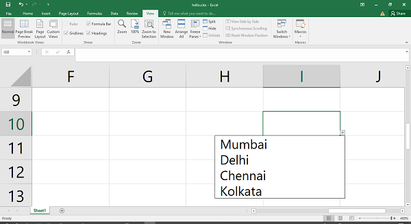
Example
If you want to make the user enter a string of length greater than 5, use >= as criteria and value set to 5.
import xlsxwriter

wb = xlsxwriter.Workbook('hello.xlsx')
worksheet = wb.add_worksheet()

worksheet.data_validation(
   'I10',{
      'validate': 'length',
      'criteria': '>=','value': 5,'input_title': 'Enter name:',
      'input_message': 'Minimum length 5 character',
      'error_message':'Name should have at least 5 characters'
   }
)

wb.close()
Output
If the string is having less than 5 characters, the error message pops up as follows −
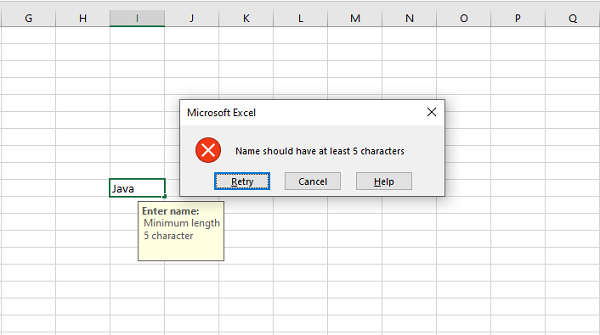
Python XlsxWriter — Outlines & Grouping
In Excel, you can group rows or columns having same value of a particular column (or row)) so that they can be hidden or displayed with a single mouse click. This feature is called to as outlines and grouping. It helps in displaying sub-totals or summaries. This feature can be found in MS excel software’s Data→Outline group.
To use this feature, the data range must have all rows should be in the sorted order of values in one column. Suppose we have sales figures of different items. After sorting the range on name of item, click on the Subtotal option in the Outline group. Following dialog box pops up.
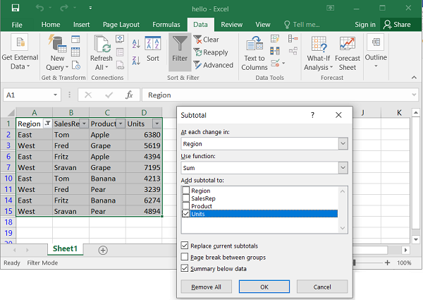
The worksheet shows item-wise subtotal of sales and at the end the grand total. On the left of the worksheet, the outline levels are shown. The original data is at level 3, the subtotals at level 2 and grand total at level 1.
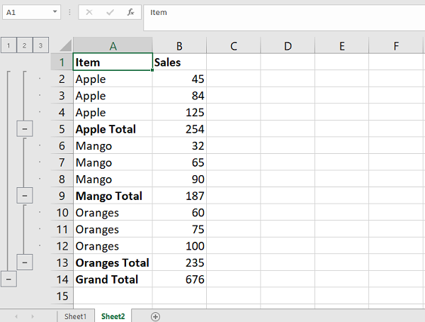
Working with Outlines and Grouping
To do this using XlsxWriter, we need to use the level property of the set_row() method. The data rows are set at level 2.
ws.set_row(row, None, None, {'level': 2})
The rows for subtotal are having level 1.
ws.set_row(row, None, None, {'level': 1})
We use SUBTOTAL() function to calculate and display the sum of sales figures in one group.
Example
The complete code is given below −
import xlsxwriter
wb = xlsxwriter.Workbook('hello.xlsx')
ws = wb.add_worksheet()

headings=['Item', 'Sales']
data=[
   ['Apple', 45], ['Apple', 84], ['Apple', 125],
   ['Mango', 32], ['Mango', 65], ['Mango', 90],
   ['Oranges', 60], ['Oranges', 75], ['Oranges',100],
]
ws.write_row('A1', headings)
item='Apple'
rownum=1
startrow=1
for row in data:
   if row[0]==item:
      ws.set_row(rownum, None, None, {'level': 2})
      ws.write_row(rownum,0, row)
      rownum+=1
else:
   ws.set_row(rownum, None, None, {'level': 1})
   ws.write(rownum, 0, item+' Subtotal')
   cellno='B{}:B{}'.format(startrow,rownum)
   print (cellno)
   ws.write(rownum,1,'=SUBTOTAL(9,'+cellno+')')
   # rownum+=1
   item=data[rownum][0]
   rownum+=1
   ws.set_row(rownum, None, None, {'level': 2})
   ws.write_row(rownum,0, row)
   rownum+=1
   startrow=rownum
else:
   ws.set_row(rownum, None, None, {'level': 1})
   ws.write(rownum, 0, item+' Subtotal')
   cellno='B{}:B{}'.format(startrow,rownum)
   ws.write(rownum,1,'=SUBTOTAL(9,'+cellno+')')
rownum+=1
ws.write(rownum, 0, 'Grand Total')
cellno='B{}:B{}'.format(1,rownum)
ws.write(rownum,1,'=SUBTOTAL(9,'+cellno+')')

wb.close()
Output
Run the code and open hello.xlsx using Excel. As we can see, the outlines are displayed on the left.
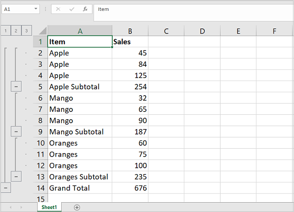
At each level, the minus sign indicates that the rows can be collapsed and only the subtotal row will be displayed.
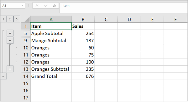
This figure shows all rows at level 2 have been collapsed. It now shows plus symbol in the outline which means that the data rows can be expanded. If you click the minus symbol at level 1, only the grand total will remain on the worksheet.
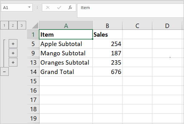
Python XlsxWriter — Freeze & Split Panes
The freeze_panes() method
The freeze_panes() method of Worksheet object in XlsxWriter library divides or splits the worksheet into horizontal or vertical regions known as panes, and «freezes» either or both of these panes so that if we scroll down or scroll down or scroll towards right, the panes (top or left respectively) remains stationary.
The method requires the parameters row and col to specify the location of the split. It should be noted that the split is specified at the top or left of a cell and that the method uses zero based indexing. You can set one of the row and col parameters as zero if you do not want either a vertical or horizontal split.
Example
The worksheet in the following example displays incrementing multiples of the column number in each row, so that each cell displays product of row number and column number.
import xlsxwriter

wb = xlsxwriter.Workbook('hello.xlsx')
worksheet = wb.add_worksheet()
format1=wb.add_format({'bg_color':'#D9D9D9', 'bold':True})

for col in range(0, 15):
   worksheet.write(0, col, col+1, format1)

for row in range(1, 51):
   for col in range(0,15):
      if col==0:
         worksheet.write(row,col,(col+1)*(row + 1), format1)
      else:
         worksheet.write(row,col,(col+1)*(row + 1))
# Freeze pane on the top row.
worksheet.freeze_panes(1, 0)

wb.close()
Output
We then freeze the top row pane. As a result, after opening the worksheet, if the cell pointer is scrolled down, the top row always remains on the worksheet.
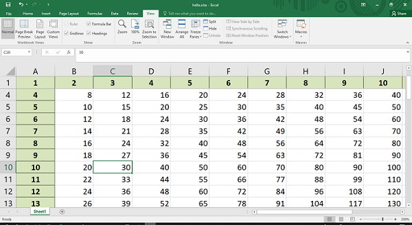
Similarly, we can make the first column stationery.
# Freeze pane on the first column.
worksheet.freeze_panes(0, 1)
The following screenshot shows that column A remains visible even if we scroll towards the right.
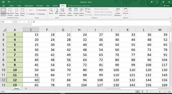
By setting row and column parameter in freeze_panes() method to 1, both the top row and leftmost column will freeze.
# Freeze pane on the first row, first column.
worksheet.freeze_panes(1, 1)
Open the resulting worksheet and scroll the cell cursor around. You will find that row and column numbers in top row and leftmost column, which have been formatted in bold and with a background color, are visible always.
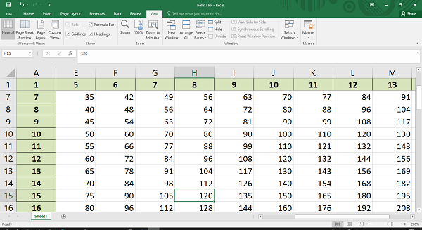
The split_panes() method
The split_panes() method also divides the worksheet into horizontal or vertical regions known as panes, but unlike freeze_panes() method, the splits between the panes will be visible to the user and each pane will have its own scroll bars.
The method has the parameters «y» and «x» that are used to specify the vertical and horizontal position of the split. These parameters are in terms of row height and column width used by Excel. The row heights and column widths have default values as 15 for a row and 8.43 for a column.
You can set one of the «y» and «x» parameters as zero if you do not want either a vertical or horizontal split.
To create a split at the 10th row and 7th column, the split_panes() method is used as follows −
worksheet.split_panes(15*10, 8.43*7)
You will find the splitters at 10th row and 7th column of the worksheet. You can scroll the panes to the left and right of vertical splitter and to the top and bottom of horizontal splitter. Note that the other panes will remain constant.
Example
Here’s the complete code that creates the splitter, and below that the output is shown −
import xlsxwriter

wb = xlsxwriter.Workbook('hello.xlsx')
worksheet = wb.add_worksheet()
format1=wb.add_format({'bg_color':'#D9D9D9', 'bold':True})

for col in range(0, 15):
   worksheet.write(0, col, col+1, format1)

for row in range(1, 51):
   for col in range(0,15):
      if col==0:
         worksheet.write(row,col,(col+1)*(row + 1), format1)
      else:
         worksheet.write(row,col,(col+1)*(row + 1))
worksheet.split_panes(15*10, 8.43*7)

wb.close()
Output
Run the code and open hello.xlsx using Excel. As we can see, the worksheet is split into different panes at 10th row and 7th column.
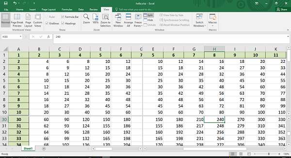
Python XlsxWriter — Hide/Protect Worksheet
The worksheet object’s hide() method makes the worksheet disappear till it is unhidden through Excel menu.
In the following worksheet, there are three sheets, of which sheet2 is hidden.
sheet1 = workbook.add_worksheet()
sheet2 = workbook.add_worksheet()
sheet3 = workbook.add_worksheet()

# Hide Sheet2. It won't be visible until it is unhidden in Excel.
worksheet2.hide()
It will create the following worksheet −
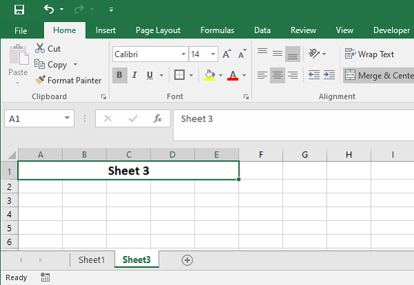
You can’t hide the «active» worksheet, which generally is the first worksheet, since this would cause an Excel error. So, in order to hide the first sheet, you will need to activate another worksheet.
sheet2.activate()
sheet1.hide()
Hide Specific Rows or Columns
To hide specific rows or columns in a worksheet, set hidden parameter to 1 in set_row() or set_column() method. The following statement hides the columns C, D and E in the active worksheet.
worksheet.set_column('C:E', None, None, {'hidden': 1})
Example
Consider the following program −
import xlsxwriter

wb = xlsxwriter.Workbook('hello.xlsx')
worksheet = wb.add_worksheet()
format1=wb.add_format({'bg_color':'#D9D9D9', 'bold':True})

for col in range(0, 15):
   worksheet.write(0, col, col+1, format1)

for row in range(1, 51):
   for col in range(0,15):
      if col==0:
         worksheet.write(row,col,(col+1)*(row + 1), format1)
      else:
         worksheet.write(row,col,(col+1)*(row + 1))
worksheet.set_column('C:E', None, None, {'hidden': 1})

wb.close()
Output
As a result of executing the above code, the columns C, D and E are not visible in the worksheet below −
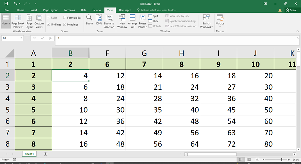
Similarly, we can hide rows with set_row() method with the help of hidden parameter.
for row in range(5, 7):
   worksheet.set_row(row, None, None, {'hidden':1})
Here is the result −
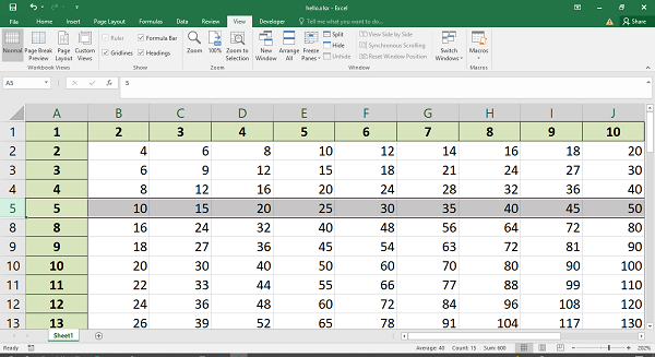
Python XlsxWriter — Textbox
In Excel, a text box is a graphic object that can be placed anywhere on the worksheet, and can be moved around if needed. Desired formatting features such as font (color, size, name etc.), alignment, fill effects, orientation etc. can be applied on the text contained in the text box.
Working with XlsxWriter – Textbox
In XlsxWriter, there is insert_textbox() method to place text box on the worksheet. The cell location of the text box and the text to be written in it must be given. Additionally, different formatting options are given in the form of a dictionary object.
Example
The following code displays a text box at cell C5, the given string is displayed with font and alignment properties as shown below −
import xlsxwriter

wb = xlsxwriter.Workbook('hello.xlsx')
worksheet = wb.add_worksheet()
text = 'Welcome to TutorialsPoint'

options = {'font': {'color': 'red','size': 14},
   'align': {'vertical': 'middle','horizontal': 'center'}}
worksheet.insert_textbox('C5', text, options)

wb.close()
Output
Open the worksheet ‘hello.xlsx‘ with Excel app. The text box appears as below −
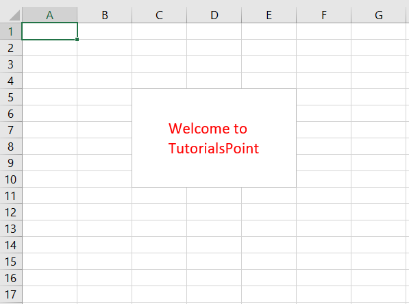
Textbox Options – fill
The text box is by default 192X120 pixels in size (corresponds to 3 columns and 6 rows). This size can be changed with width and height parameters, both given in pixels. One of the parameters acceptable to inset_textbox() method is the fill parameter. It takes a predefined color name or color representation in hexadecimal as value.
Example
The following code displays a multi-line string in the custom sized text box having background filled with red color.
import xlsxwriter
wb = xlsxwriter.Workbook('hello.xlsx')
worksheet = wb.add_worksheet()
text = 'TutorialsPoint - Simple Easy LearningnThe best resource for Online Education'

options = {
   'width': 384,
   'height':80,
   'font': {'color': 'blue', 'bold':True, 'size': 14},
   'align': {'vertical': 'middle', 'horizontal': 'center'},
   'fill':{'color':'red'},
}
worksheet.insert_textbox('C5', text, options)
wb.close()
As we can see in the figure below, a text box with multiple lines is rendered at cell C5.
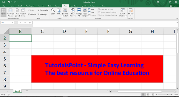
Textbox Options – text_rotation
Another important property is the text_rotation. By default, the text appears horizontally. If required, you may change its orientation by giving an angle as its value. Look as the following options.
import xlsxwriter
wb = xlsxwriter.Workbook('hello.xlsx')
worksheet = wb.add_worksheet()
text = 'TutorialsPoint - Simple Easy LearningnThe best resource for Online Education'

options = {
   'width': 128,
   'height':200,
   'font': {'bold':True, 'name':'Arial', 'size': 14},
   'text_rotation':90,
}
worksheet.insert_textbox('C5', text, options)
wb.close()
The text now appears in the text box with its vertical orientation.
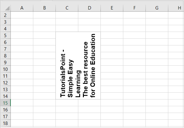
The object_position parameter controls the behaviour of the text box. It can have the following possible values and their effect −
-
«1» − Move and size with cells (the default).
-
«2» − Move but don’t size with cells.
-
«3» − Don’t move or size with cells.
Python XlsxWriter — Insert Image
It is possible to insert an image object at a certain cell location of the worksheet, with the help of insert_image() method. Basically, you have to specify the location of cell using any type of notation and the image to be inserted.
worksheet.insert_image('C5', 'logo.png')
The insert_image() method takes following optional parameters in a dictionary.
| Parameter | Default |
|---|---|
| ‘x_offset’ | 0, |
| ‘y_offset’ | 0, |
| ‘x_scale’ | 1, |
| ‘y_scale’ | 1, |
| ‘object_position’ | 2, |
| ‘image_data’ | None |
| ‘url’ | None |
| ‘description’ | None |
| ‘decorative’ | False |
The offset values are in pixels. The x_scale and y_scale parameters are used to scale the image horizontally and vertically.
The image_data parameter is used to add an in-memory byte stream in io.BytesIO format.
Example
The following program extracts the image data from a file in the current folder and uses is as value for image_data parameter.
from io import BytesIO
import xlsxwriter
workbook = xlsxwriter.Workbook('hello.xlsx')
worksheet = workbook.add_worksheet()

filename = 'logo.png'

file = open(filename, 'rb')
data = BytesIO(file.read())
file.close()

worksheet.insert_image('C5', filename, {'image_data': data})

workbook.close()
Output
Here is the view of the resultant worksheet −
Python XlsxWriter — Page Setup
The worksheet page setup methods are related to appearance of the worksheet when it is printed. These worksheet methods control the orientation, paper size, margins, etc.
set_landscape()
This method is used to set the orientation of a worksheet’s printed page to landscape.
set_portrait()
This method is used to set the orientation of a worksheet’s printed page to portrait. This is the default orientation.
set_page_view()
This method is used to display the worksheet in «Page View/Layout» mode.
set_paper()
This method is used to set the paper format for the printed output of a worksheet. It takes index as an integer argument. It is the Excel paper format index.
Following are some of the paper styles and index values −
| Index | Paper format | Paper size |
|---|---|---|
| 0 | Printer default | Printer default |
| 1 | Letter | 8 1/2 x 11 in |
| 2 | Letter Small | 8 1/2 x 11 in |
| 3 | Tabloid | 11 x 17 in |
| 4 | Ledger | 17 x 11 in |
| 5 | Legal | 8 1/2 x 14 in |
| 6 | Statement | 5 1/2 x 8 1/2 in |
| 7 | Executive | 7 1/4 x 10 1/2 in |
| 8 | A3 | 297 x 420 mm |
| 9 | A4 | 210 x 297 mm |
set_margin()
This method is used to set the margins of the worksheet when it is printed. It accepts left, right, top and bottom parameters whose values are in inches. All parameters are optional The left and right parameters are 0.7 by default, and top and bottom are 0.75 by default.
Python XlsxWriter — Header & Footer
When the worksheet is printed using the above methods, the header and footer are generated on the paper. The print preview also displays the header and footer. Both are configured with set_header() and set_footer() methods. Header and footer string is configured by following control characters −
| Control | Category | Description |
|---|---|---|
| &L | Justification | Left |
| &C | Center | |
| &R | Right | |
| &P | Information | Page number |
| &N | Total number of pages | |
| &D | Date | |
| &T | Time | |
| &F | File name | |
| &A | Worksheet name | |
| &Z | Workbook path | |
| &fontsize | Font | Font size |
| &»font,style» | Font name and style | |
| &U | Single underline | |
| &E | Double underline | |
| &S | Strikethrough | |
| &X | Superscript | |
| &Y | Subscript | |
| &[Picture] | Images | Image placeholder |
| &G | Same as &[Picture] | |
| && | Misc. | Literal ampersand «&» |
Example
The following code uses set_header() and set_footer() methods −
import xlsxwriter

wb = xlsxwriter.Workbook('hello.xlsx')
ws = wb.add_worksheet()

data = [
   ['Anil', 45, 55, 50], ['Ravi', 60, 70, 80],
   ['Kiran', 65, 75, 85],['Karishma', 55, 65, 45]
]

for row in range(len(data)):
   ws.write_row(row,0, data[row])

header1 = '&CTutorialspoint'
footer1 = '&LSimply Easy Learning'

ws.set_landscape()
ws.set_paper(9) #A4 paper
ws.set_header(header1)
ws.set_footer(footer1)

ws.set_column('A:A', 50)

wb.close()
Output
Run the above Python code and open the worksheet. From File menu, choose Print option. On the right pane, the preview is shown. You should be able to see the header and footer.
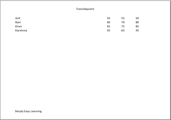
Python XlsxWriter — Cell Comments
In an Excel worksheet, comments can be inserted for various reasons. One of the uses is to explain a formula in a cell. Also, Excel comments also serve as reminders or notes for other users. They are useful for cross-referencing with other Excel workbooks.
From Excel’s menu system, comment feature is available on Review menu in the ribbon.
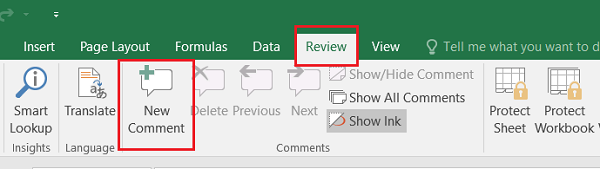
To add and format comments, XlsxWriter has add_comment() method. Two mandatory parameters for this method are cell location (either in A1 type or row and column number), and the comment text.
Example
Here is a simple example −
import xlsxwriter

wb = xlsxwriter.Workbook('hello.xlsx')
ws = wb.add_worksheet()

data='XlsxWriter Library'

ws.set_column('C:C', 25)
ws.set_row(2, 50)
ws.write('C3', data)

text = 'Developed by John McNamara'
ws.write_comment('C3', text)

wb.close()
Output
When we open the workbook, a comment will be seen with a marker on top right corner of C3 cell when the cursor is placed in it.
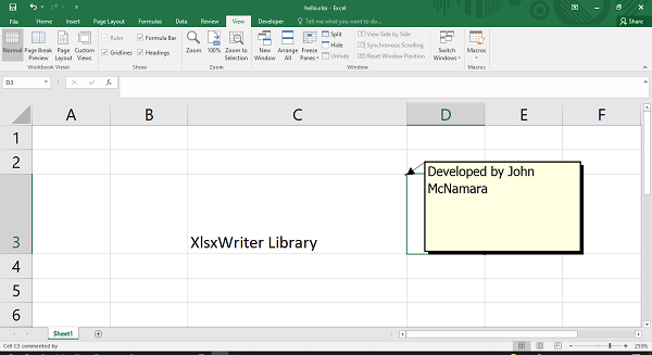
By default, the comments are not visible until the cursor hovers on the cell in which the comment is written. You can either show all the comments in a worksheet by invoking show_comment() method of worksheet object, or setting visible property of individual comment to True.
ws.write_comment('C3', text, {'visible': True})
Example
In the following code, there are three comments placed. However, the one in cell C3 is has been configured with visible property set to False. Hence, it cannot be seen until the cursor is placed in the cell.
import xlsxwriter

wb = xlsxwriter.Workbook('hello.xlsx')
ws = wb.add_worksheet()

ws.show_comments()

data='Python'
ws.set_column('C:C', 25)
ws.set_row(0, 50)
ws.write('C1', data)
text = 'Programming language developed by Guido Van Rossum'
ws.write_comment('C1', text)
data= 'XlsxWriter'
ws.set_row(2, 50)
ws.write('C3', data)
text = 'Developed by John McNamara'
ws.write_comment('C3', text, {'visible':False})
data= 'OpenPyXl'
ws.set_row(4, 50)
ws.write('C5', data)
text = 'Developed by Eric Gazoni and Charlie Clark'
ws.write_comment('C5', text, {'visible':True})

wb.close()
Output
It will produce the following output −
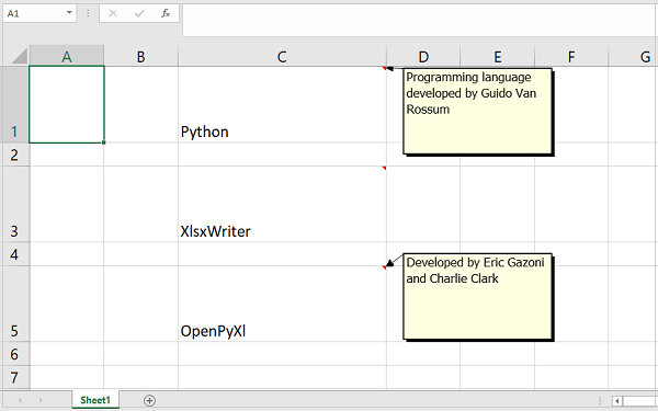
You can set author option to indicate who is the author of the cell comment. The author of the comment is also displayed in the status bar at the bottom of the worksheet.
worksheet.write_comment('C3', 'Atonement', {'author': 'Tutorialspoint'})
The default author for all cell comments can be set using the set_comments_author() method −
worksheet.set_comments_author('Tutorialspoint')
It will produce the following output −
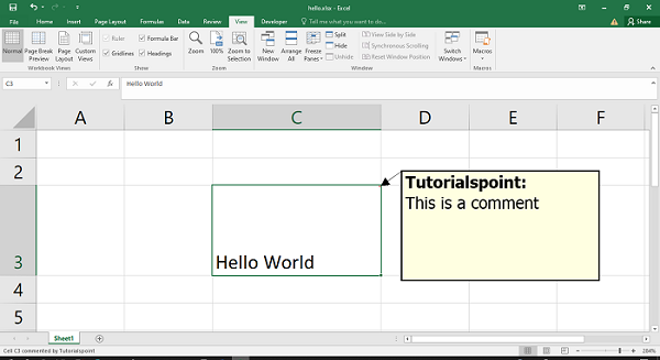
Python XlsxWriter — Working with Pandas
Pandas is a popular Python library for data manipulation and analysis. We can use XlsWriter for writing Pandas dataframes into an Excel worksheet.
To learn the features described in this section, we need to install Pandas library in the same environment in which XlsxWriter has been installed.
pip3 install pandas
Using XlsxWriter with Pandas
Let us start with a simple example. First, create a Pandas dataframe from the data from a list of integers. Then use XlsxWriter as the engine to create a Pandas Excel writer. With the help of this engine object, we can write the dataframe object to Excel worksheet.
Example
import pandas as pd

df = pd.DataFrame({'Data': [10, 20, 30, 20, 15, 30, 45]})
writer = pd.ExcelWriter('hello.xlsx', engine='xlsxwriter')
df.to_excel(writer, sheet_name='Sheet1')

writer.save()
Output
The worksheet so created shows up as follows −
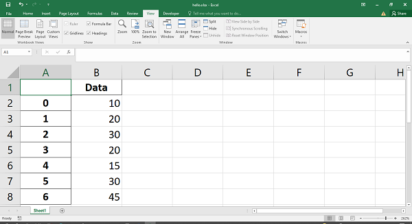
Adding Charts to Pandas Dataframe
Just as we obtain an object of Workbook class, and then a Worksheet object by calling its add_worksheet() method, the writer object can also be used to fetch these objects. Once we get them, the XlsxWriter methods to add chart, data table etc. can be employed.
In this example, we set up a Pandas dataframe and obtain its dimension (or shape).
import pandas as pd
df = pd.DataFrame({'Data': [105, 60, 35, 90, 15, 30, 75]})
writer = pd.ExcelWriter('hello.xlsx', engine='xlsxwriter')
df.to_excel(writer, sheet_name='Sheet1')
(max_row, max_col) = df.shape
The workbook and worksheet objects are created from the writer.
workbook = writer.book
worksheet = writer.sheets['Sheet1']
Rest of things are easy. The chart object is added as we have done earlier.
chart = workbook.add_chart({'type': 'column'})
chart.add_series({'values': ['Sheet1', 1, 1, max_row, 1]})
worksheet.insert_chart(1, 3, chart)
writer.save()
Example
The following code uses Pandas dataframe to write an Excel workbook and a column chart is prepared by XlsxWriter.
import pandas as pd

df = pd.DataFrame({'Data': [105, 60, 35, 90, 15, 30, 75]})
writer = pd.ExcelWriter('hello.xlsx', engine='xlsxwriter')
df.to_excel(writer, sheet_name='Sheet1')
(max_row, max_col) = df.shape

workbook = writer.book
worksheet = writer.sheets['Sheet1']
chart = workbook.add_chart({'type': 'column'})
chart.add_series({'values': ['Sheet1', 1, 1, max_row, 1]})
worksheet.insert_chart(1, 3, chart)

writer.save()
Output
The column chart along with the data is shown below −
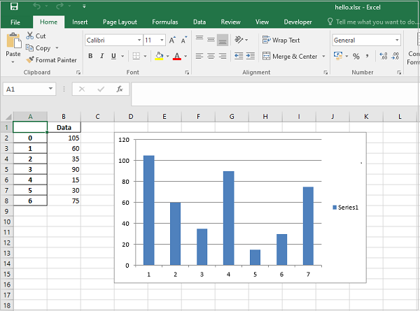
Writing Dataframe to Excel Table
Similarly, the dataframe can be written to Excel table object. The dataframe here is derived from a Python dictionary, where the keys are dataframe column headers. Each key has list as a value which in turn becomes values of each column.
import pandas as pd

df = pd.DataFrame({
   'Name': ['Namrata','Ravi','Kiran','Karishma'],
   'Percent': [73.33, 70, 75, 65.5],
   'RollNo': [1, 2,3,4]})

df = df[['RollNo', 'Name', 'Percent']]
(max_row, max_col) = df.shape
Use xlsxwriter engine to write the dataframe to a worksheet (sheet1)
writer = pd.ExcelWriter('hello.xlsx', engine='xlsxwriter')
df.to_excel(writer, sheet_name='Sheet1', startrow=1, header=False, index=False)
Following lines give Workbook and Worksheet objects.
workbook = writer.book
worksheet = writer.sheets['Sheet1']
Data in the worksheet is converted to Table with the help of add_table() method.
column_settings = [{'header': column} for column in df.columns]

worksheet.add_table(0, 0, max_row, max_col - 1, {'columns': column_settings})

writer.save()
Example
Below is the complete code to write pandas dataframe to Excel table.
import pandas as pd
df = pd.DataFrame({
   'Name': ['Namrata','Ravi','Kiran','Karishma'],
   'Percent': [73.33, 70, 75, 65.5],
   'RollNo': [1, 2,3,4]
})

df = df[['RollNo', 'Name', 'Percent']]
(max_row, max_col) = df.shape

writer = pd.ExcelWriter('hello.xlsx', engine='xlsxwriter')
df.to_excel(writer, sheet_name='Sheet1', startrow=1, header=False, index=False)

workbook = writer.book
worksheet = writer.sheets['Sheet1']

column_settings = [{'header': column} for column in df.columns]

worksheet.add_table(0, 0, max_row, max_col - 1, {'columns': column_settings})

writer.save()
Output
The Table using default autofilter settings appears at A1 cell onwards.
Python XlsxWriter — VBA Macro
In Excel, a macro is a recorded series of steps that can be repeated any number of times with a shortcut key. The steps performed while recording the macro are translated into programming instructions VBA which stands for Visual Basic for Applications. VBA is a subset of Visual basic language, especially written to automate the tasks in MS Office apps such as Word, Excel, PowerPoint etc.
The option to record a macro is available in the Developer menu of MS Excel. If this menu is not seen, it has to be activated by going to the «File→Options→Customize» ribbon screen.
As shown in the following figure, click the Record Macro button by going to «View→Macros→Record Macro», and give a suitable name to the macro and perform desired actions to be recorded. After the steps are over stop the recording. Assign a desired shortcut so that the recorded action can be repeated as and it is pressed.
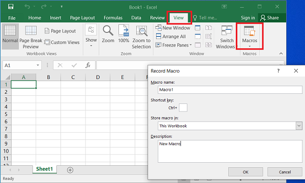
To view the VBA code, edit the macro by going View→ZMacros→View Macros. Select the Macro from Macro name and click on Edit.
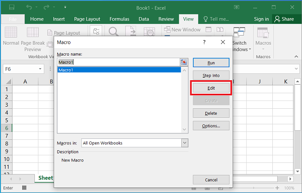
The VBA editor will be shown. Delete all the steps generated by Excel and add the statement to pop-up a message box.
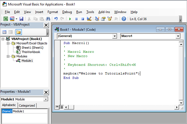
Confirm that the macro works perfectly. Press CTL+Shift+M and the message box pops up. Save this file with the .xlsm extension. It internally contains vbaproject.bin, a binary OLE COM container. To extract it from the Excel macro file, use the vba_extract.py utility.
(xlsxenv) E:xlsxenv>vba_extract.py test.xlsm
Extracted: vbaProject.bin
Example
This vbaProject.bin file can now be added to the XlsxWriter workbook using the add_vba_project() method. On this worksheet, place a button object at B3 cell, and link it to the macro that we had already created (i.e., macro1)
import xlsxwriter

workbook = xlsxwriter.Workbook('testvba.xlsm')
worksheet = workbook.add_worksheet()

worksheet.set_column('A:A', 30)
workbook.add_vba_project('./vbaProject.bin')
worksheet.write('A3', 'Press the button to say Welcome.')
worksheet.insert_button(
   'B3',
   {
      'macro': 'macro1',
      'caption': 'Press Me',
      'width': 80, 'height': 30
   }
)
workbook.close()
Output
When the above code is executed, the macro enabled workbook named testvba.xlsm will be created. Open it and click on the button. It will cause the message box to pop up as shown.
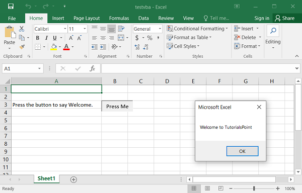
Python Excel Writer: Create, Write(Text, Number, Formula), Modify, Save, Apply settings, Merge- unmerge cells and more

With
the help of openpyxl module we can also write to excel file in python.
The process is somewhat similar to reading an excel spreadsheet in
python. With python Excel writer, we will Create excel sheets, write text, numbers and formula in cells. After modifying we will save workbook. We will also add and delete sheets in a an excel workbook, apply setting, fonts and styles, set width and height of cells and areas, merge and unmerge cells. We can create any type of excel file, having hundreds
and thousands of columns and rows of data. Writing to excel files is a
necessity which no one can deny. There may be many cases for all
professionals from a computer operator to a data scientist that one has
to write to an excel spreadsheet in python. Here is the solution.
If you want to Read, Write and Manipulate(Copy, cut, paste, delete or search for an item or value etc) Excel files in Python with simple and practical examples I will suggest you to see this simple and to the point
Python Excel Openpyxl Course with examples about how to deal with MS Excel files in Python. This video course teaches efficiently how to manipulate excel files and automate tasks.
Everything you do in Microsoft Excel, can be automated with Python. So why not use the power of Python and make your life easy. You can make intelligent and thinking Excel sheets, bringing the power of logic and thinking of Python to Excel which is usually static, hence bringing flexibility in Excel and a number of opportunities.
Automate your Excel Tasks and save Time and Effort. You can save dozens or hundreds of hours by Python Excel Automation with just a single click get your tasks done with in seconds which used to take hours of Manual Excel and Data Entry Work.
Python Excel Create and Save files:
First we will learn how to create and save excel files with python.
First we will create an excel file.
First step will be to import openpyxl
module.
>>> import openpyxl
Next we will create an excel file or
technically a Workbook.
>>> mywb =
openpyxl.Workbook()
The above code will create a work book with one sheet in the beginning.
We can check the number of sheets with the following code, see which
sheet is active and what is the title of the active sheet. In this case
we have only one sheet, hence it will be the only answer.
>>>
mywb.get_sheet_names()
[‘Sheet’]
>>> sheet =
mywb.active
>>> sheet.title
‘Sheet’
We can also set the title of the
sheet, see the example given below.
>>>
sheet.title = ‘MyNewTitle’
>>>
wb.get_sheet_names()
[‘MyNewTitle’]
>>>mywb.save(‘NewExcelFile.xlsx’)
If you open your root folder or
current working directory, you will find a new excel file, with name
NewExcelFile, having one sheet with title MyNewTitle.
Loading an already existing excel file in Python and saving a
copy of it:
Whenever you load an already existing Excel file in memory, and modify
the contents, either sheets or cells, or creating whole sheets, or
deleting sheets, or any modification which could be done, you will have
to call save( ) method to save the file. If you don’t do so, any
modification will be lost.
>>> import openpyxl
>>>
mywb = openpyxl.load_workbook(‘filetest.xlsx’)
>>>
sheet = mywb.active
>>>
sheet.title = ‘Working on Save as’
>>>
mywb.save(‘example_filetest.xlsx’)
In the code above you noticed that we
loaded already existing file, changed sheet title and saved its copy
with a different name. In this case original file plus this new file
will be in your working directory, which is usually your python root
folder. Open it and see the new copy.
When you work on an excel spreadsheet
in python, its always better to save it with a different file name, so
that the original is always there, in case any mishap happens, for
example any bug in code, or mistake in saving, or writing.
Creating and Removing Sheets in Excel:
For creating new sheets in a
workbook, we use create_sheet( ) method.
For deleting a sheet we use
remove_sheet( ) method.
>>>
import
openpyxl
>>> mywb =
openpyxl.Workbook()
>>> mywb.get_sheet_names()
[‘Sheet’]
>>>
mywb.create_sheet()
<Worksheet «Sheet1»>
>>> mywb.get_sheet_names()
[‘Sheet’, ‘Sheet1’]
>>>
wb.create_sheet(index=0, title=’1st
Sheet’)
<Worksheet «1st Sheet»>
>>>
mywb.get_sheet_names()
[‘1st Sheet’, ‘Sheet’, ‘Sheet1’]
>>>mywb.create_sheet(index=2,
title=’2nd
Sheet’)
<Worksheet «2nd Sheet»>
>>>mywb.get_sheet_names()
[‘1st Sheet’, ‘Sheet’, ‘2nd Sheet’,
‘Sheet1’]
Create sheet creates a new sheet,
which is by default the last sheet in the workbook. However, we can
specify the position of the new sheet with index number and we can also
pass a string as the title of new sheet. Keep in mind, the first sheet
will have index 0, second will have index 1 and so on.
Removing sheets from Excel Workbook:
When we want to remove any specific
sheet from an excel workbook, we will use method remove_sheet( )
>>>mywb.get_sheet_names()
[‘1st Sheet’, ‘Sheet’, ‘2nd Sheet’,
‘Sheet1’]
This is to see the number of sheets and their names, now working with
removing or deleting sheets.
>>>
mywb.remove_sheet(mywb.get_sheet_by_name(‘1st Sheet’))
>>>
mywb.remove_sheet(mywb.get_sheet_by_name(‘Sheet1’))
>>>
mywb.get_sheet_names()
[‘Sheet’, ‘2nd Sheet’]
It is very obvious that after
deleting the two sheets from four sheets, only two sheets are left.
remove_sheet method takes a worksheet object not name of the sheet,
instead of creating an object to that specific worksheet and then
removing it, we call get_sheet_by_name( ) and pass it the name of
sheet, the value it returns is the input argument of remove_sheet( )
method. In the end, use save( ) method to save the file after
modification. In this case removal of worksheets.
Python excel Writing Values in Cells:
Now we will see how to write values
to particular cells in an excel worksheet. Ofcourse we should know the
address of the cell where we want to write.
>>> import openpyxl
>>> mywb =
openpyxl.Workbook()
>>> mysheet =
mywb.get_sheet_by_name(‘Sheet’)
>>> mysheet[‘F6’] =
‘Writing new Value!’
>>> mysheet[‘F6’].value
‘Writing new Value’
Python Excel setting Fonts:
Applying different styles to your
sheet, emphasizes or stresses certain rows or columns. It is very
important to apply certain uniform styles to your excel sheets so that
it brings clarity in reading the data. If you have hundreds or
thousands of rows of data, styling can be a hectic job, however, with
our python code, you can write a few lines of code and apply on
millions of lines of data instantly. But take care, first styling
should be with absolute care, and second always save excel workbook
with a different name.
First we will import openpyxl, and then import Font and Style for use
in our code.
Here’s an example that creates a new
workbook and sets cell F6 to have a 32-point, italicized font.
>>>
import
openpyxl
>>>
from
openpyxl.styles import Font, Style
>>>
mywb
= openpyxl.Workbook()
>>>
mysheet
= mywb.get_sheet_by_name(‘Sheet’)
>>>
italic32Font = Font(size=32, italic=True)
>>>
sobj = Style(font=italic24Font)
>>>
mysheet[‘F6’].style = sobj
>>>
mysheet[‘F6’]
= ‘Applying Styles!’
>>>
mywb.save(‘Appliedstyle.xlsx’)
In openpyxl for excel worksheets each
cell has a style object which is in style attribute of the cell. We
create a style object and assign it to style attribute.
There are four arguments for Font objects
- Name: A string value is used, quoting the font name, like
‘Arial’. - Size: An integer value, quoting the size.
- Bold: A boolean value, True for Bold font.
- Italic: Boolean value, True for Italic font.
In the example below we will call Font( ) method to create a Font
object and store it in a variable, next step will be to pass that as an
argument to Style( ) method. We will store the that object in another
variable and assign it to the specific cell object.
>>> import openpyxl
>>> from
openpyxl.styles import Font, Style
>>> mywb =
openpyxl.Workbook()
>>> mysheet =
mywb.get_sheet_by_name(‘Sheet’)
>>> firstFontObj =
Font(name=’Arial’,
bold=True)
>>> firstStyleObj =
Style(font=firstFontObj)
>>>
mysheet[‘F6’].style/firstStyleObj
>>> mysheet[‘F6’] =
‘Bold Arial’
>>> secondFontObj =
Font(size=32, italic=True)
>>> secondStyleObj =
Style(font=secondFontObj)
>>>
mysheet[‘D7’].style/secondStyleObj
>>> mysheet[‘D7′] =
’32 pt Italic’
>>>
mywb.save(‘ApplicationofStyles.xlsx’)
Python Excel
Writing Formulae:
Formulae in Excel are very important, infact the power of a spreadsheet
is in its formulae. Openpyxl provides the utility of writing formula in
any specific cell. Infact it is very much easy, instead of writing a
number or text, write an equal sign followed by the required formula.
>>>mysheet[‘F6’]
= ‘=Sum(D7:D20)’
This formula will sum up all values
from D7 to D20 and store in F6 cell.
Some more examples:
>>> import openpyxl
>>> mywb =
openpyxl.Workbook()
>>> mysheet =
mywb.active
>>> mysheet[‘F6’] =
500
>>> mysheet[‘F7’] =
800
>>> sheet[‘D3’] =
‘=SUM(F6:F7)’
>>>
mywb.save(‘Applyingformula.xlsx’)
In the above example we put 500 in
F6, and 800 in F7 cell. Cell D3 has a formula of adding up F6 and F7.
When you will open spreadsheet, it will show a value of 1300 in D3.
The cells in A1 and A2 are set to 200
and 300, respectively.
The value in cell A3 is set to a formula that sums the values in A1 and
A2.
When the spreadsheet is opened in Excel, A3 will display its value as
500.
Excel Adjusting Rows and Columns in a Sheet:
We can set Row heigh, column width in excel spreadsheet using openpyxl.
We can also freeze rows or columns so that they always appear. We can
also hide rows or columns.
>>> import openpyxl
>>> mywb =
openpyxl.Workbook()
>>> mysheet =
mywb.active
>>> mysheet[‘F6’] =
‘Tall row’
>>> mysheet[‘D7’] =
‘Wide column’
>>> mysheet.row_dimensions[3].height
= 65
>>>mysheet.column_dimensions[‘F’].width
= 25
>>>mywb.save(‘Heightandwidth.xlsx’)
The
default row height in excel spreadsheet is 12.75 points. Where one
point is equal to 1/72 of an inch. You can set a value between 0 to 409.
Column width can be set to a value from 0 to 255. It can be either an
integer or a floating value (decimal number). If you set 0 width for
column or 0 height for rows, it will be hidden.
Excel Merging and unmerging
openpyxl allows us to merge and
unmerge cells in a workbook.
>>> import openpyxl
>>>my wb =
openpyxl.Workbook()
>>> mysheet =
mywb.active
>>>
mysheet.merge_cells(‘B2:D3’)
>>> mysheet[‘A1’] =
‘cells merged
together.’
>>> mysheet.merge_cells(‘F6:F7’)
>>> mysheet[‘G5’] =
‘Two merged cells.’
>>> mywb.save(‘Mergingcells.xlsx’)
merge_cells method takes two cell
addresses as its arguments. First cell is the top left and second cell
is the right bottom of the rectangular area that is to be merged. If we
want to set value of that merged area, we use the address of top left
cell of the whole merged area.
If you want to unmerge cells, use the
idea below.
>>> import openpyxl
>>> mywb =
openpyxl.load_workbook(‘Mergingcells.xlsx’)
>>> mysheet =
mywb.active
>>>
mysheet.unmerge_cells(‘B2:D3’)
>>> mysheet.unmerge_cells(‘F6:F7’)
>>> mywb.save(‘unmerged.xlsx’)
If you want to Read, Write and Manipulate(Copy, cut, paste, delete or search for an item or value etc) Excel files in Python with simple and practical examples I will suggest you to see this simple and to the point
Python Excel Openpyxl Course with examples about how to deal with MS Excel files in Python. This video course teaches efficiently how to manipulate excel files and automate tasks.
Everything you do in Microsoft Excel, can be automated with Python. So why not use the power of Python and make your life easy. You can make intelligent and thinking Excel sheets, bringing the power of logic and thinking of Python to Excel which is usually static, hence bringing flexibility in Excel and a number of opportunities.
Automate your Excel Tasks and save Time and Effort. You can save dozens or hundreds of hours by Python Excel Automation with just a single click get your tasks done with in seconds which used to take hours of Manual Excel and Data Entry Work.