Protected functions in excel

Watch Video – How to Lock Formulas in Excel

Excel formulas are easy to create and edit in Excel.

You can easily edit a formula through the formula bar or directly in the cell.

While this makes it convenient to create formulas in Excel, it comes with a few disadvantages as well.

Consider this.

You are going through a worksheet full of formulas, and you accidentally hit the delete key, or backspace key, or some other number/alphabet key.

Now you’ll be lucky if you’re able to spot the error and correct it. But if you are not, it may lead to some erroneous results.

And let me tell you this, errors in Excel have cost millions to companies (read this or this).

The chances of such errors increase multifold when you share a file with colleagues or managers or clients.

One of the ways to prevent this from happening is to lock the worksheet and all the cells. However, doing this would prevent the user from making any changes to the worksheet. For example, if you’re sending a workbook to your manager for review, you may want to allow him to add his comments or change some cells.

A better workaround to this is to lock only those cells that have formulas in it.

How to Lock Formulas in Excel

Before I show you how to lock formulas in Excel, here is something you must know:

By default, all the cells are locked in Excel. Only when you protect the locked cells can you truly restrict the user from making changes. This also means that if a cell is not locked and you protect it, the user would be able to make changes.

Here are the steps to lock formulas in Excel (explained in detail later on):

Select all the cells and unlock these.
Select all the cells that have formulas (using Go To Special).
Lock these selected cells.
Protect the worksheet.

Now that I have outlined the steps above, let’s dive in and see how to do this (and more importantly, why we must do this):

Step 1: Select All the Cells and Unlock it

While you may find it confusing, bear with me and keep reading.

As I mentioned, only the cells that are locked as well as protected can truly be restricted. If all the cells are locked, and I protect the entire worksheet, it would mean a user can’t change anything.

But we only want to lock (restrict access) to the cells that have formulas in it.

To do this, we first need to unlock all the cells and then select and lock only those cells that have formulas in it.

Here are the steps to unlock all the cells:

Step 2: Select All the Cells that Have Formulas

Now that all the cells have been unlocked, we need to make sure that the cells that have formulas are locked.

To do this, we need to first select all the cells with formulas.

Here are the steps to select all the cells that have formulas:

This would select all the cells that have formulas in it.

Step 3: Lock the Cells with Formulas

Now that we have selected the cells with formulas, we need to go back and lock these cells (enable the lock property that we disabled in step 1).

Once we do this, protecting the worksheet would lock these cells that have formulas, but not the other cells.

Here are the steps to Lock Cells with Formulas:

Step 4 – Protect the Worksheet

Now that the ‘Locked’ property is enabled for cells with formulas (and not for other cells), protecting the entire worksheet would only restrict access to the cells with formulas.

Here are the steps to protect the worksheet:

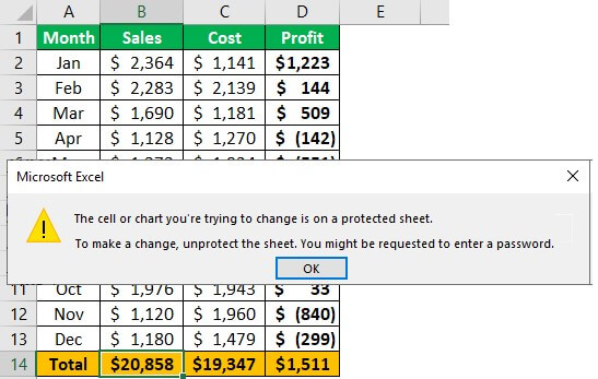
Once you are done with the above four steps, all the cells that have formulas would be locked, and the user wouldn’t be able to change anything in it.

If the user tries to change the cells, he/she will get a prompt as shown below:

How to Hide Formulas in Excel

When you lock formulas in Excel, the user can’t make any changes to the cells with formulas.

However, if that cell is selected, the formula in the cell would be visible in the formula bar.

While this isn’t an issue in most cases, but if you don’t want the formula to be visible, you need to hide it.

Here are the steps to hide formulas in locked cells:

Now, when the user selects a cell that has a formula and is locked, he/she will not be able to see the formula in the formula bar.

Note: As mentioned earlier, a cell that has not been locked cannot be protected. The same applies when you hide formulas in Excel. Unless the cell is locked, only checking the Hidden checkbox wouldn’t do anything. To truly hide formulas in Excel, the cells should have the Locked and Hidden check boxes selected, and then it should be protected.

You May Also Like the Following Excel Tutorials:

Lock Rows/Columns using Excel Freeze Panes.
How to Copy and Paste Formulas in Excel without Changing Cell References.
Show Formulas in Excel Instead of the Values.
How to Convert Formulas to Values in Excel.
Unhide Columns in Excel
How to Lock Row Height & Column Width in Excel

Источник

Excel Lock Formula (Table of Contents)

Lock Formula in Excel
How to Lock and Protect Formulas in excel?

Lock Formula in Excel

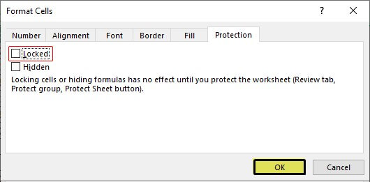
To protect our work or functional formula in Excel, we can lock the sheet or workbook to protect that. There are different ways to do it. The first way, select the Protect Sheet option from the Review menu tab under the Changes section. Next, please choose the option which we want to lock in a workbook, then give the password to lock it. In another way, we can lock any cell’s formula using Format cell. Click right on the cell which we want to protect, and from the Format Cells option, select LOCKED from the protection tab.

How to Lock and Protect Formulas?

It is a very simple and easy task to lock and protect formulas. Let’s understand how to lock and protect the formulas with an example.

You can download this Lock Formulas Excel Template here – Lock Formulas Excel Template

Excel Lock Formula – Example #1

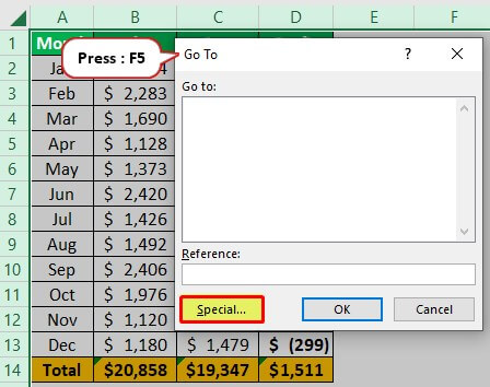
Consider the below example, which shows the data of the sales team members.

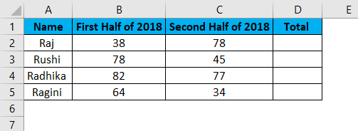
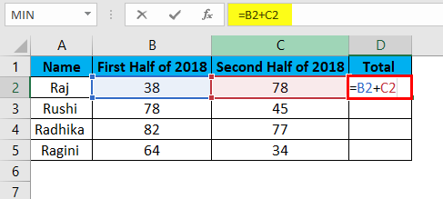
In the below image, in column D, the total has been calculated by inserting the formula =B2+C2 in cell D2.

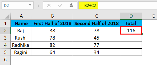
The Result will be as shown below:

The formula in the total column has been copied from cells D2:D5.

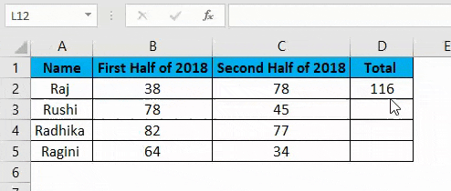
In this example, we are going to lock the formula entered in column D. So, let us see the steps to lock and protect the formulas.

Please select all the cells by pressing Ctrl+A and unlock them.
Select the cells or the entire columns or rows where you need to apply the formula.
Lock the cells which contain the formula.
Protect the worksheet.

Let us in detail show how are the above steps executed.

Step 1: Unlocking all the cells

The cells in excel are protected and locked in excel. As we need to lock particular cells in the workbook, it is necessary to unlock all the cells. So let us see how to unlock all the cells. The steps to unlock all the cells are as follows:

Press Ctrl+A to select the entire worksheet.
Right, Click, and select Format Cells from the options that appeared in the context menu.

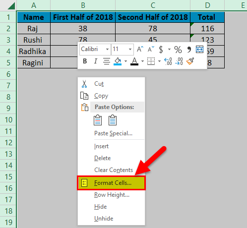
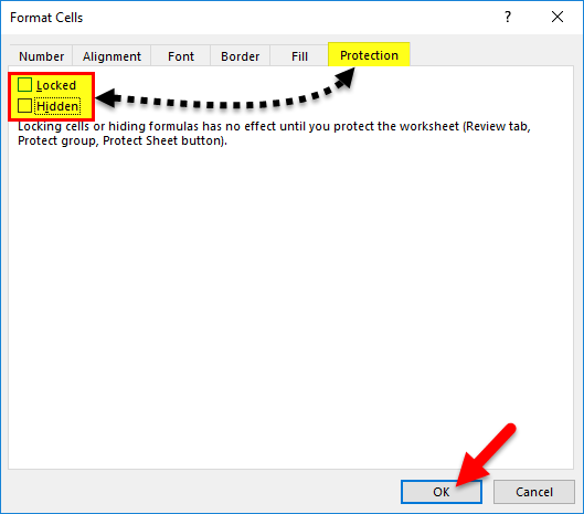
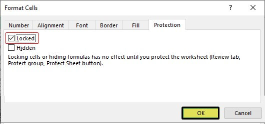
Select the Protection tab and uncheck the Locked and Hidden option as well and then click OK.

Step 2: Select and lock the cells containing the formula

Now here we need to lock the cells where we have entered the formula. The steps to lock the cells containing formula in excel are as follows:

Select all the cells in the worksheet by pressing Ctrl +A.
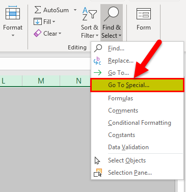
Go to the Home tab and select Find & Select option from the Editing menu.

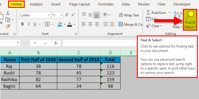
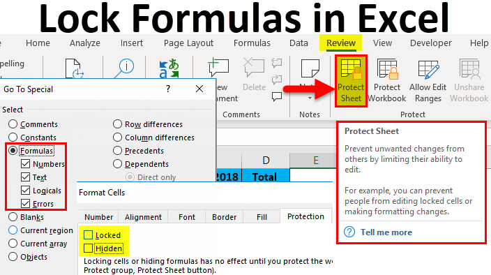
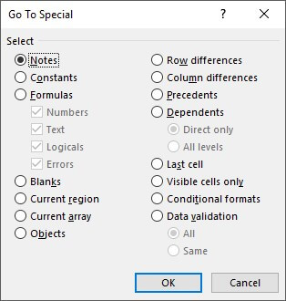
After selecting the Find & Select option, other options will appear under it, from which select the Go To Special option.

Go To Special dialog box will appear as shown below.

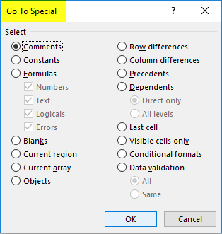
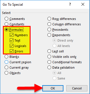
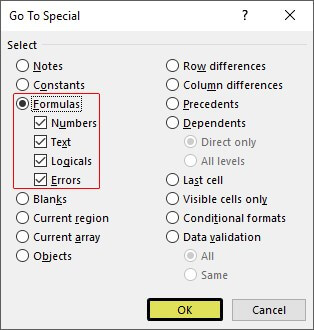
We have to select the Formulas option and check all the options under the Formulas button are ticked and then click OK.

Step 3: Protection of the Worksheet

This function is used to ensure that locked property is enabled not only for cells with formulas but also for all the cells in the workbook. Let us see the steps followed to implement the protection for the worksheet:

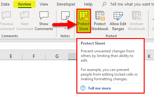
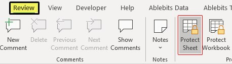
First, go to the Review tab and select Protect Sheet option.

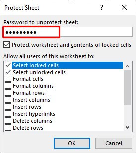
After this, the Protect Sheet dialog box will appear.

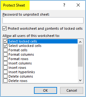
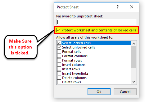
In which make sure that “Protect Worksheet and contents of locked cells” is selected.

The user can also type a password in the text box under the Password to unprotect the sheet in order to make the worksheet safer.

Advantages of Lock Formulas in Excel

It helps the user to keep their data secure from others when they send their files to other recipients.
It helps the user to hide their work when the file is shared with other readers and users.
The user can use a password in the case to protect the entire workbook, which can be written in the text box named, ‘Password to unprotect the sheet.’

Disadvantages of Lock Formulas in Excel

A new user won’t be able to understand the function in excel easily.
It becomes difficult if the user forgets to enter the password to unprotect the file.
It is sometimes not an efficient way in terms of time as it consumes the time of a user to protect and unprotect the cells of the worksheet.

Things to Remember

All the cells are protected by default, do not forget to unlock the cells in order to lock formulas in excel.
After locking formulas in excel, make sure to lock the worksheet again.
The entire workbook can be protected by using the option restricted or unrestricted access from the “Protect Workbook” option.
In case if the user needs to hide their work or formulas from others, they can tick the option “Hidden” by selecting the “Protection” tab from the “Format Cells” dialog box.
In case the user needs to unprotect the complete file, simply type the password by selecting the “Unprotect Sheet” option.
A user can save time by moving the formulas to separate worksheets and then hiding them instead of wasting time protecting and unprotecting the worksheet.

How to Protect Formulas in Excel?

Protection is the key to excelling and sharing the same Excel workbook with others. So the protection of formulas is part of Excel’s worksheets protection. Therefore, we need to follow simple steps to protect our formulas.

You can download this Protect Formulas Excel Template here – Protect Formulas Excel Template

For example, look at the below data in Excel.

All the black-colored cells are formula cells in the above table, so we need to protect them. Assume we need to allow the users to work with other cells except for the cells with formulas. Follow these below steps, and protect them.

By default, all the cells are locked in Excel. So, if we protect the worksheet directly, it will save all the cells, and users cannot work with any of the cells. So first, we need to unlock all the cells of the worksheet.

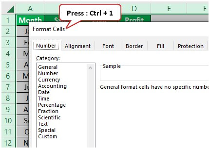
First, we must select the entire worksheet and press “Ctrl + 1” to open the “Format Cells” window.
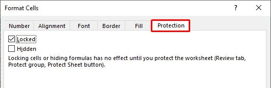
In the above window, click on the “Protection” tab.
As we can see under “Protection,” the checkbox of “Locked” is ticked. So, all the cells are clocked now. Therefore, uncheck this box.

Next, click on “OK,” and all the cells are unlocked now.
Once all the cells are unlocked, we need to lock only formula cells because we need to protect only formula cells, so how do we know which cell has the formula in it?

First, we should select the entire worksheet and press the “F5” key to open the “Go To” window and press on the “Special” tab.
Consequently, it will take us to the “Got To Special” window like the one below.
From the above window, we must choose “Formulas.”
Then, click on “OK.” As a result, all the cells which have formulas will be selected.

Look, it has selected only the black-colored font cells.
Again, we must press “Ctrl + 1” to open the “Format Cells” window. We need to make these cells locked this time, so choose “Locked.”

Then, click on “OK.” It will lock only selected cells, and protection applies only to these cells.
Now, we need to protect the worksheet to protect formulas in Excel. So, click on the “Protect Sheet” option under the “Review” tab.
In the “Protect Sheet” window, we need to enter the password to protect the locked cells, so insert the formulas we would like to give. (Ensure you remember the formula)

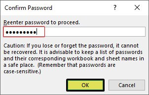
In the above window, we can choose other actions that we can perform with locked cells. So by default, the first two options are selected. If we want to give any further actions to the user, we can check those boxes. We are not allowing users to do any activity with locked cells except for selecting cells.
We must click on “OK” and reenter the password in the next window.

Click on “OK.” The formulas are now protected.

If we try to perform any action in formula cells, it will show the below message.

Like this, we can protect formulas in Excel.

How to Hide Formulas in Excel?

The formulas are protected. But, we can go one step further, i.e., we can hide formulas from viewing in the formula bar.

As of now, we can see the formula in the formula bar even after protection.

So to hide them, we must first unprotect the worksheet that we have protected. Then, choose only the formula cell and open the “Format Cells” dialog box.

Under the “Protection” tab, we must check the box “Hidden.”

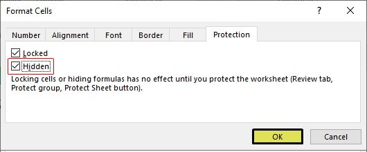
Then, click on “OK” to close the above window.

Now again, protect the worksheet. All the formula cells will not show any formulas in the formula bar.

Things to Remember

All the cells are locked by default, so only formula cells unlock other cells to protect.
To select only formula cells, we must use the “Go To Special” option (F5 is the shortcut key). Under “Go To Special,” click on “Formulas.”

So, it is important to know how to lock formula cells in Excel!

There may be situations when you have to share these files with a colleague or boss. At those times, hiding or protecting the formula will become of utmost importance.

Two methods on how to protect formula cells in Excel are:

Locking the Cells
Hiding the Formula Bar

Let’s look at each of these methods!

Locking the Cells

If you have a workbook with lots of formulas and you want to protect those formulas from being amended by other people who share your workbook, then you can even lock the cells!

Watch it on YouTube and give it a thumbs-up!

You need to follow these steps on how to lock formula cells in Excel and download the Excel Workbook below to practice along with:

STEP 1: Press the Go To Special shortcut CTRL+G.

STEP 2: Select the Constants box and press OK (this highlights all the non-formula cells)

By default, all the cells in Excel are locked. So, we need to select the cells containing constant values and unlock them.

In the end, only the cells containing formulas will remain locked!

STEP 3: Press CTRL+1 to bring up the Format Cells dialogue box

STEP 4: Select the Protection tab and Un-check the Locked box

STEP 5: In the menu ribbon go to Review > Protect Sheet > then enter your custom password (optional)

This will lock all the cells that are not constant, so all the formula cells 🙂

Now, if you try to make any change in the protected cells you will be prompted with this message and will not be able to make any edits.

This is how to protect formulas in Excel by locking the cells.

In this method, even though the cells will be locked you can still see the formula used.

To hide the formula from others, follow the second method.

Hiding the Formula Bar

An easy way to prevent a user from making an undesired change in a cell, you can hide the formula in the formula bar. Follow the steps below to do so:

STEP 1: Press the Go To Special shortcut CTRL+G.

STEP 2: Select the Formulas box and press OK (this highlights all the formula cells)

STEP 3: Press CTRL+1 to bring up the Format Cells dialogue box.

STEP 4: In the Format Cells dialogue box, go to the Protection tab and un-check the Locked box, and check the Hidden box.

STEP 5: Go to the Review Tab > Protect Sheet.

STEP 6: In the Protect Sheet dialog box, Click OK.

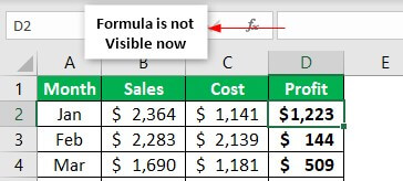
STEP 7: Select the cell C8, you will see that the formula bar is blank!

It is important to understand that the sheet needs to be protected in order to hide the formula. Simply checking the hidden box will not do the trick!

This completes our tutorial on how to protect formula in Excel!

Conclusion

If you have sensitive data in your Excel workbook that you wish to hide from others using the file, you can follow one of these two methods on how to lock formula cells in Excel.

You can even use these methods to simply protect your workbook from any unwanted and accidental change being made.

In the first method, you can prevent others from making any changes to the cells with formulas by locking the cells.

But the formula used in the cell would still be visible in the formula bar

You can follow the second method in which the formula in the cell will not be visible in the formula bar as well.

HELPFUL RESOURCE:

Make sure to download our FREE PDF on the 333 Excel keyboard Shortcuts here:

Источник

Данные в Excel можно защищать от постороннего вмешательства. Это важно, потому что иногда вы тратите много времени и сил на создание сводной таблицы или объемного массива, а другой человек случайно или намеренно изменяет либо вовсе удаляет все ваши труды.

Рассмотрим способы защиты документа Excel и его отдельных элементов.

Защита ячейки Excel от изменения

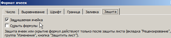
Как поставить защиту на ячейку в Excel? По умолчанию все ячейки в Excel защищаемые. Это легко проверить: кликаем на любую ячейку правой кнопкой, выбираем ФОРМАТ ЯЧЕЕК – ЗАЩИТА. Видим, что галочка на пункте ЗАЩИЩАЕМАЯ ЯЧЕЙКА проставлена. Но это еще не значит, что они уже защищены от изменений.

Зачем нам эта информация? Дело в том, что в Excel нет такой функции, которая позволяет защитить отдельную ячейку. Можно выбрать защиту листа, и тогда все ячейки на нем будут защищены от редактирования и другого вмешательства. С одной стороны это удобно, но что делать, если нам нужно защитить не все ячейки, а лишь некоторые?

Рассмотрим пример. Имеем простую таблицу с данными. Такую таблицу нам нужно разослать в филиалы, чтобы магазины заполнили столбец ПРОДАННОЕ КОЛИЧЕСТВО и отправили обратно. Во избежание внесения каких-то изменений в другие ячейки, защитим их.

Для начала освободим от защиты те ячейки, куда сотрудники филиалов будут вносить изменения. Выделяем D4:D11, правой кнопкой вызываем меню, выбираем ФОРМАТ ЯЧЕЕК и убираем галочку с пункта ЗАЩИЩАЕМАЯ ЯЧЕЙКА.

Теперь выбираем вкладку РЕЦЕНЗИРОВАНИЕ – ЗАЩИТИТЬ ЛИСТ. Появляется такое окно, где будут проставлены 2 галочки. Первую из них мы убираем, чтобы исключить любое вмешательство сотрудников филиалов, кроме заполнения столбца ПРОДАННОЕ КОЛИЧЕСТВО. Придумываем пароль и нажимаем ОК.

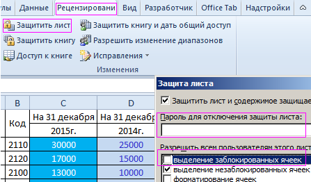
Внимание! Не забудьте свой пароль!

Теперь в диапазон D4:D11 посторонние лица смогут только вписать какое-то значение. Т.к. мы ограничили все остальные действия, никто не сможет даже изменить цвет фона. Все средства форматирования на верхней панели инструментов не активные. Т.е. они не работают.

Защита книги Excel от редактирования

Если на одном компьютере работает несколько человек, то целесообразно защищать свои документы от редактирования третьими лицами. Можно ставить защиту не только на отдельные листы, но и на всю книгу.

Когда книга будет защищена, посторонние смогут открывать документ, видеть написанные данные, но переименовать листы, вставить новый, поменять их расположение и т.п. Попробуем.

Прежнее форматирование сохраняем. Т.е. у нас по-прежнему можно вносить изменения только в столбец ПРОДАННОЕ КОЛИЧЕСТВО. Чтобы защитить книгу полностью, на вкладке РЕЦЕНЗИРОВАНИЕ выбираем ЗАЩИТИТЬ КНИГУ. Оставляем галочки напротив пункта СТРУКТУРУ и придумываем пароль.

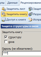
Теперь, если мы попробуем переименовать лист, у нас это не получится. Все команды серого цвета: они не работают.

Снимается защита с листа и книги теми же кнопками. При снятии система будет требовать тот же пароль.

Источник

How to Lock Formulas in Excel

Step 1: Select All the Cells and Unlock it

Step 2: Select All the Cells that Have Formulas

Step 3: Lock the Cells with Formulas

Step 4 – Protect the Worksheet

How to Hide Formulas in Excel

Lock Formula in Excel

How to Lock and Protect Formulas?

Excel Lock Formula – Example #1

Step 1: Unlocking all the cells

Step 2: Select and lock the cells containing the formula

Step 3: Protection of the Worksheet

Advantages of Lock Formulas in Excel

Disadvantages of Lock Formulas in Excel

Things to Remember

Recommended Articles

Table of contents

How to Protect Formulas in Excel?

How to Hide Formulas in Excel?

Things to Remember

Recommended Articles

So, it is important to know how to lock formula cells in Excel!

Locking the Cells

Hiding the Formula Bar

Conclusion

Защита ячейки Excel от изменения

Защита книги Excel от редактирования