
By default, protecting a worksheet locks all cells so none of them are editable. To enable some cell editing, while leaving other cells locked, it’s possible to unlock all the cells. You can lock only specific cells and ranges before you protect the worksheet and, optionally, enable specific users to edit only in specific ranges of a protected sheet.
Lock only specific cells and ranges in a protected worksheet
Follow these steps:
-
If the worksheet is protected, do the following:
-
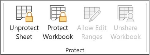
On the Review tab, click Unprotect Sheet (in the Changes group).

Click the Protect Sheet button to Unprotect Sheet when a worksheet is protected.
-
If prompted, enter the password to unprotect the worksheet.
-
-
Select the whole worksheet by clicking the Select All button.
-
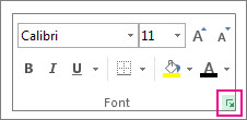
On the Home tab, click the Format Cell Font popup launcher. You can also press Ctrl+Shift+F or Ctrl+1.
-
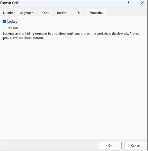
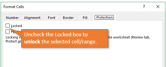
In the Format Cells popup, in the Protection tab, uncheck the Locked box and then click OK.
This unlocks all the cells on the worksheet when you protect the worksheet. Now, you can choose the cells you specifically want to lock.
-
On the worksheet, select just the cells that you want to lock.
-
Bring up the Format Cells popup window again (Ctrl+Shift+F).
-
This time, on the Protection tab, check the Locked box and then click OK.
-
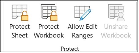
On the Review tab, click Protect Sheet.
-
In the Allow all users of this worksheet to list, choose the elements that you want users to be able to change.
More information about worksheet elements
Clear this check box
To prevent users from
Select locked cells
Moving the pointer to cells for which the Locked check box is selected on the Protection tab of the Format Cells dialog box. By default, users are allowed to select locked cells.
Select unlocked cells
Moving the pointer to cells for which the Locked check box is cleared on the Protection tab of the Format Cells dialog box. By default, users can select unlocked cells, and they can press the TAB key to move between the unlocked cells on a protected worksheet.
Format cells
Changing any of the options in the Format Cells or Conditional Formatting dialog boxes. If you applied conditional formats before you protected the worksheet, the formatting continues to change when a user enters a value that satisfies a different condition.
Format columns
Using any of the column formatting commands, including changing column width or hiding columns (Home tab, Cells group, Format button).
Format rows
Using any of the row formatting commands, including changing row height or hiding rows (Home tab, Cells group, Format button).
Insert columns
Inserting columns.
Insert rows
Inserting rows.
Insert hyperlinks
Inserting new hyperlinks, even in unlocked cells.
Delete columns
Deleting columns.
If Delete columns is protected and Insert columns is not also protected, a user can insert columns that he or she cannot delete.
Delete rows
Deleting rows.
If Delete rows is protected and Insert rows is not also protected, a user can insert rows that he or she cannot delete.
Sort
Using any commands to sort data (Data tab, Sort & Filter group).
Users can’t sort ranges that contain locked cells on a protected worksheet, regardless of this setting.
Use AutoFilter
Using the drop-down arrows to change the filter on ranges when AutoFilters are applied.
Users cannot apply or remove AutoFilters on a protected worksheet, regardless of this setting.
Use PivotTable reports
Formatting, changing the layout, refreshing, or otherwise modifying PivotTable reports, or creating new reports.
Edit objects
Doing any of the following:
-
Making changes to graphic objects including maps, embedded charts, shapes, text boxes, and controls that you did not unlock before you protected the worksheet. For example, if a worksheet has a button that runs a macro, you can click the button to run the macro, but you cannot delete the button.
-
Making any changes, such as formatting, to an embedded chart. The chart continues to be updated when you change its source data.
-
Adding or editing comments.
Edit scenarios
Viewing scenarios that you have hidden, making changes to scenarios that you have prevented changes to, and deleting these scenarios. Users can change the values in the changing cells, if the cells are not protected, and add new scenarios.
Chart sheet elements
Select this check box
To prevent users from
Contents
Making changes to items that are part of the chart, such as data series, axes, and legends. The chart continues to reflect changes made to its source data.
Objects
Making changes to graphic objects — including shapes, text boxes, and controls — unless you unlock the objects before you protect the chart sheet.
-
-
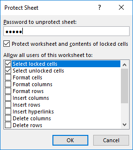
In the Password to unprotect sheet box, type a password for the sheet, click OK, and then retype the password to confirm it.
-
The password is optional. If you do not supply a password, any user can unprotect the sheet and change the protected elements.
-
Make sure that you choose a password that is easy to remember, because if you lose the password, you won’t have access to the protected elements on the worksheet.
-

Unlock ranges on a protected worksheet for users to edit
To give specific users permission to edit ranges in a protected worksheet, your computer must be running Microsoft Windows XP or later, and your computer must be in a domain. Instead of using permissions that require a domain, you can also specify a password for a range.
-
Select the worksheet that you want to protect.
-
On the Review tab, in the Changes group, click Allow Users to Edit Ranges.
This command is available only when the worksheet is not protected.
-
Do one of the following:
-
To add a new editable range, click New.
-
To modify an existing editable range, select it in the Ranges unlocked by a password when sheet is protected box, and then click Modify.
-
To delete an editable range, select it in the Ranges unlocked by a password when sheet is protected box, and then click Delete.
-
-
In the Title box, type the name for the range that you want to unlock.
-
In the Refers to cells box, type an equal sign (=), and then type the reference of the range that you want to unlock.
You can also click the Collapse Dialog button, select the range in the worksheet, and then click the Collapse Dialog button again to return to the dialog box.
-
For password access, in the Range password box, type a password that allows access to the range.
Specifying a password is optional when you plan to use access permissions. Using a password allows you to see user credentials of any authorized person who edits the range.
-
For access permissions, click Permissions, and then click Add.
-
In the Enter the object names to select (examples) box, type the names of the users who you want to be able to edit the ranges.
To see how user names should be entered, click examples. To verify that the names are correct, click Check Names.
-
Click OK.
-
To specify the type of permission for the user who you selected, in the Permissions box, select or clear the Allow or Deny check boxes, and then click Apply.
-
Click OK two times.
If prompted for a password, type the password that you specified.
-
In the Allow Users to Edit Ranges dialog box, click Protect Sheet.
-
In the Allow all users of this worksheet to list, select the elements that you want users to be able to change.
More information about the worksheet elements
Clear this check box
To prevent users from
Select locked cells
Moving the pointer to cells for which the Locked check box is selected on the Protection tab of the Format Cells dialog box. By default, users are allowed to select locked cells.
Select unlocked cells
Moving the pointer to cells for which the Locked check box is cleared on the Protection tab of the Format Cells dialog box. By default, users can select unlocked cells, and they can press the TAB key to move between the unlocked cells on a protected worksheet.
Format cells
Changing any of the options in the Format Cells or Conditional Formatting dialog boxes. If you applied conditional formats before you protected the worksheet, the formatting continues to change when a user enters a value that satisfies a different condition.
Format columns
Using any of the column formatting commands, including changing column width or hiding columns (Home tab, Cells group, Format button).
Format rows
Using any of the row formatting commands, including changing row height or hiding rows (Home tab, Cells group, Format button).
Insert columns
Inserting columns.
Insert rows
Inserting rows.
Insert hyperlinks
Inserting new hyperlinks, even in unlocked cells.
Delete columns
Deleting columns.
If Delete columns is protected and Insert columns is not also protected, a user can insert columns that he or she cannot delete.
Delete rows
Deleting rows.
If Delete rows is protected and Insert rows is not also protected, a user can insert rows that he or she cannot delete.
Sort
Using any commands to sort data (Data tab, Sort & Filter group).
Users can’t sort ranges that contain locked cells on a protected worksheet, regardless of this setting.
Use AutoFilter
Using the drop-down arrows to change the filter on ranges when AutoFilters are applied.
Users cannot apply or remove AutoFilters on a protected worksheet, regardless of this setting.
Use PivotTable reports
Formatting, changing the layout, refreshing, or otherwise modifying PivotTable reports, or creating new reports.
Edit objects
Doing any of the following:
-
Making changes to graphic objects including maps, embedded charts, shapes, text boxes, and controls that you did not unlock before you protected the worksheet. For example, if a worksheet has a button that runs a macro, you can click the button to run the macro, but you cannot delete the button.
-
Making any changes, such as formatting, to an embedded chart. The chart continues to be updated when you change its source data.
-
Adding or editing comments.
Edit scenarios
Viewing scenarios that you have hidden, making changes to scenarios that you have prevented changes to, and deleting these scenarios. Users can change the values in the changing cells, if the cells are not protected, and add new scenarios.
Chart sheet elements
Select this check box
To prevent users from
Contents
Making changes to items that are part of the chart, such as data series, axes, and legends. The chart continues to reflect changes made to its source data.
Objects
Making changes to graphic objects — including shapes, text boxes, and controls — unless you unlock the objects before you protect the chart sheet.
-
-
In the Password to unprotect sheet box, type a password, click OK, and then retype the password to confirm it.
-
The password is optional. If you do not supply a password, then any user can unprotect the worksheet and change the protected elements.
-
Ensure that you choose a password that you can remember. If you lose the password, you will be unable to access to the protected elements on the worksheet.
-
If a cell belongs to more than one range, users who are authorized to edit any of those ranges can edit the cell.
-
If a user tries to edit multiple cells at once and is authorized to edit some but not all of those cells, the user will be prompted to edit the cells one-by-one.
Need more help?
You can always ask an expert in the Excel Tech Community or get support in the Answers community.
Bottom Line: Learn how to lock individual cells or ranges in Excel so that users cannot change the formulas or contents of protected cells. Plus a few bonus tips to save time with the setup.
Skill Level: Beginner
Video Tutorial
Download the Excel File
You can download the file that I use in the video tutorial by clicking below.
Protecting Your Work from Unwanted Changes
If you share your spreadsheets with other users, you’ve probably found that there are specific cells you don’t want them to modify. This is especially true for cells that contain formulas and special formatting.
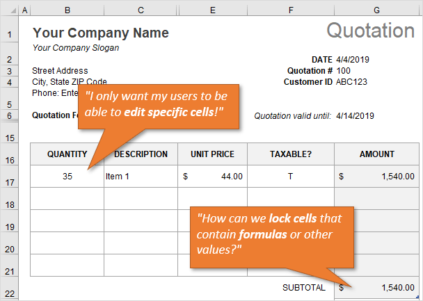
The great news is that you can lock or unlock any cell, or a whole range of cells, to keep your work protected. It’s easy to do, and it involves two basic steps:
- Locking/unlocking the cells.
- Protecting the worksheet.
Here’s how to prevent users from changing some cells.
Step 1: Lock and Unlock Specific Cells or Ranges
Right-click on the cell or range you want to change, and choose Format Cells from the menu that appears.
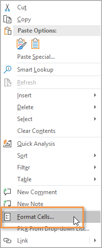
This will bring up the Format Cells window (keyboard shortcut for this window is Ctrl + 1.). Choose the tab that says Protection.
Next, make sure that the Locked option is checked.
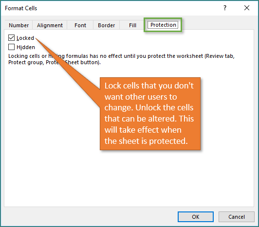
Locked is the default setting for all cells in a new worksheet/workbook.
Once we protect the worksheet (in the next step) those locked cells will not be able to be altered by users.
If you want users to be able to edit a particular cell or range, uncheck the Locked box so they are unlocked. Since cells are locked by default, most of the job will be going through the sheet and unlocking cells that can be edited by users.
I share some shortcuts to make this process faster in the Bonus section below.
Step 2: Protect the Worksheet
Now that you’ve locked/unlocked the cells that you want users to be able to edit, you want to protect the sheet. Once you protect the sheet, users cannot change the locked cells. However, they can still modify the unlocked cells.
To protect the sheet, simply right-click on the tab at the bottom of the sheet, and choose Protect Sheet… from the menu.
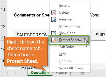
This will bring up the Protect Sheet window. If you want your sheet to be password protected, you have the option of entering a password here. Adding a password is optional. Click OK.
If you’ve chosen to enter a password, then you will be prompted to verify your entry after you’ve clicked OK.
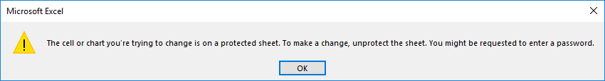
With the sheet protected, users will be unable to change the cells that are locked. If they try to make changes, they will get an error/warning message that looks like this.
You can unprotect the sheet in the same way that you protected it, by right-clicking on the sheet tab. An alternative way to protect and unprotect sheets is by using the Protect Sheet button in the Review tab of the Ribbon.
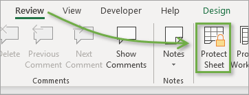
The button text displays the opposite of the current state. It says Protect Sheet when the sheet is unprotected, and Unprotect Sheet when it is protected.
It’s important to note that all cells can be edited when the sheet is unprotected. After making changes you must protect the sheet again and Save the workbook before sending or sharing with other users.
3 Bonus Tips for Locking Cells and Protecting Sheets
As you can see, it is fairly simple to protect your formulas and formatting from being changed! But I’d like to leave you with three tips to help make it faster & easier for both you and your users.
1. Prevent Locked Cells From Being Selected
This tip will help make it faster and easier for your users to input data in the sheet.
Turning off the Select locked cells option prevents the locked cells from being selected with either the mouse or keyboard (arrow or tab keys). This means users will only be able to select the unlocked cells that they need to edit. They can quickly hit the Tab, Enter, or arrow keys to move to the next editable cell.
To make this change, you just uncheck the option that says “Select locked cells” on the Protect Sheet window.
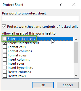
After pressing OK, you will only be able to select the unlocked cells.
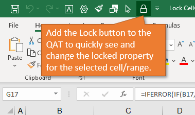
2. Add a button for locking cells to the Quick Access Toolbar
This allows you to quickly see the locked setting for a cell or range.
From the Home tab on the Ribbon, you can open the drop-down menu under the Format button and see the option to Lock Cell.
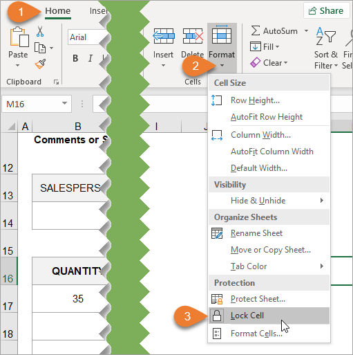
If you right-click on the Lock Cell option, another menu appears giving you the option to add the button to the Quick Access Toolbar.
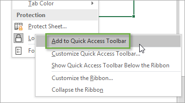
When you select this option, the button will be added to the Quick Access Toolbar at the top of the workbook. This button will remain each time you use Excel. You can easily lock and unlock specific cells on your sheet by clicking on this button.
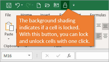
You can also see if the active cell locked or unlocked. The button will have a dark background if the selection is locked.
It’s important to note that this only shows the locked state of the active cell. If you have multiple cells selected, the active cell is the cell you selected first and appears with no fill shading.
Mixed Lock State
If you select a range that contains both locked and unlocked cells, you will see a solid box for the Locked checkbox in the Format Cells window. This denotes the mixed state.
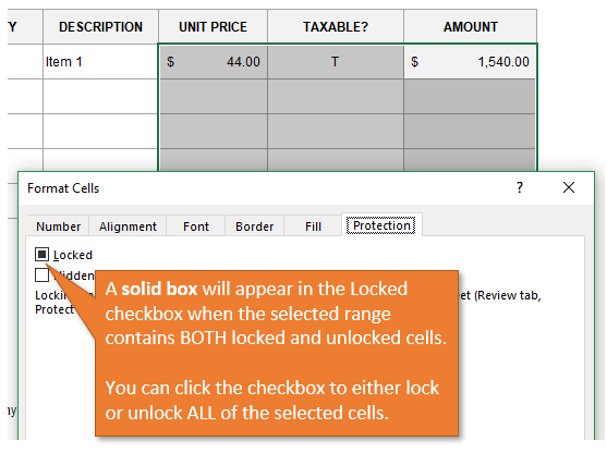
You can click the checkbox to lock or unlock ALL cells in the selected range.
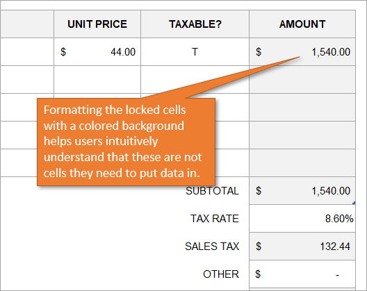
3. Use different formatting for locked cells
By changing the formatting of cells that are locked, you give your users a visual clue that those cells are off limits. In this example the locked cells have a gray fill color. The unlocked (editable) cells are white. You can also provide a guide on the sheet or instructions tab.
You might be wondering where I found this template for a quote. I got it from the template library. You can access the library by going to the File tab, choosing New, and using the search word “quote.”
You can find all sorts of useful templates there, including invoices, calendars, to-do lists, budgets, and more.
Conclusion
By locking your cells and protecting your sheet, you can keep your formulas safe from tampering by other users, and prevent mistakes.
I hope this simple tutorial proves helpful to you. Please leave a comment below if you have any tips or questions about locking cells, protecting sheets with passwords, or preventing users from changing cells.
Thank you! 🙂
Содержание
- Сдвигаем границу строки
- Одновременное скрытие нескольких строк
- Используем контекстное меню
- Применяем кнопки на ленте
- Группировка
- Панель инструментов
- Фильтр
- С помощью возможностей «Условное форматирование»
- Настройка правильных параметров в «Настройках» программы
- При помощи настроек цвета и параметров печати
- Скрытие помеченных строк/столбцов макросом
- Скрытие строк/столбцов с заданным цветом
- Выборочная защита диапазонов для разных пользователей
- Защита листов книги
- Блокировка через рецензирование
- Заморозка ячейки
- Закрепление области
- Фиксация формулы в Excel по вертикали
- Полезные советы
- Как скрыть формулу заблокированной ячейки
- Снимаем защиту
- Заключение
Сдвигаем границу строки
Данный метод, пожалуй, является самым простым. И вот, в чем он заключается.
- На вертикальной координатной панели наводим указатель мыши на нижнюю границу строки, которую планируем скрыть. Когда появится знак в виде плюсика со стрелками вверх и вниз, зажав левую кнопку мыши тянем его вверх, соединив с верхней границей строки.

- Таким нехитрым способом нам удалось скрыть выбранную строку.


Одновременное скрытие нескольких строк
Этот способ базируется на том, который мы рассмотрели выше, и также предполагает сдвиг границы, но не отдельной строки, а выделенного диапазона.
- На вертикальной координатной панели любым удобным способом (например, с помощью зажатой левой кнопки мыши) выделяем строки, которые планируем спрятать.Если требуется выделить разрозненные строки, выполняем выделение левой кнопкой мыши (щелчком или зажав для идущих подряд строк), удерживая клавишу Ctrl на клавиатуре.
- Аналогично скрытию одной строки (действия описали в методе выше), сдвигаем границу любой строки из выделенного диапазона. При этом неважно, тянем ли мы указатель к верхней границе именно этой строки или к границе самой верхней строки отмеченной области.
- В итоге мы скрыли сразу весь выделенный диапазон.


Используем контекстное меню
Наверное, это самый популярный способ среди пользователей, который предполагает использование контекстного меню.
- На вертикальной панели координат выделяем нужные строки (как это сделать, описано выше).
- Щелкаем правой кнопкой мыши по любому месту в выделенном диапазоне на координатной панели, в открывшемся списке выбираем команду “Скрыть”.

- Весь выделенный диапазон строк будет спрятан.


Применяем кнопки на ленте
На ленте программы также, предусмотрены кнопки для скрытия строк.
- Для начала нужно выделить строки, которые мы планируем спрятать. Сделать это можно по-разному:
- Находясь во вкладке “Главная” в группе инструментов “Ячейки” щелкаем по кнопке “Формат”. В открывшемся перечне выбираем команду “Скрыть или отобразить”, затем – “Скрыть строки”.

- Получаем скрытый диапазон строк.


Группировка
Чтобы скрыть ячейки с плюсом, необходимо воспользоваться специальным инструментом Excel – группировка. Он расположен во вкладке Данные на Панели инструментов в блоке Структура.

Порядок действий следующий:
- Выделяете необходимую область

- Переходите во вкладку Данные и нажимаете кнопку Группировать.

- Сбоку от выделенного участка появилась специальная скобочка и знак минус. Нажав по нему, строки скроются, а сигналом сгруппированных ячеек будет небольшой плюсик.

- Чтобы посмотреть скрытую область, нажимаете на плюс и таблица примет первоначальный вид.
На заметку! С помощью этой функции можно делать сложную группировку с несколькими вложениями, каждое из которых будет зависеть от вышестоящей группы.


Для того, чтобы убрать группировку, необходимо в той же вкладке нажать кнопку Разгруппировать, предварительно выделив сгруппированный участок.

Панель инструментов
Аналогичную операцию можно сделать через главную вкладку. Для этого ищете кнопку Формат и из выпадающего списка выбираете строку Скрыть или отобразить. Далее выбираете нужное действие.

Чтобы отобразить ячейки обратно, выбираете в том же меню функцию Отобразить строки или столбцы, в зависимости от того, что скрывалось.

Фильтр
Фильтрация данных еще один способ сокрытия информации. Ставите курсор в нужную ячейку, переходите к блоку Редактирование на Главной вкладке, нажимаете кнопку Сортировка и фильтр, потом из выпадающего списка выбираете Фильтр. Если все сделано правильно, в ячейке появится стрелочка вниз.

Нажав на этот флажок, убираете галочки с нужных позиций, затем подтверждаете действие кнопкой ОК.

Таблица приняла другой вид, а о применении фильтрации свидетельствует синий цвет номеров строк и небольшая воронка вместо стрелочки.

Отличительной особенностью этого метода является то, что полученную информацию можно скопировать без скрытых ячеек.

С помощью возможностей «Условное форматирование»
Для того чтобы узнать, как скрыть значение ячеек также можно использовать возможности «Условного форматирования». Для этого нам нужно выделить диапазон ячеек, где мы будем скрывать значения с нулевым результатом. Выбираем вкладку «Главная», блок «Стили», нажимаем иконку «Условное форматирование», в списке который раскрылся, выбираете «Правила выделение ячеек – Равно…». Следующим этапом станет указать какой именно формат вам будет надо, в поле «Форматировать ячейки, которые РАВНЫ:» устанавливаете значение 0. В открывшемся списке выбираете «Пользовательский формат…»,

в диалоговом окне «Формат ячеек» переходим на вкладку «Шрифт», потом в списке меню «Цвет» вы изменяете «Цвет темы: Авто» на «Цвет темы: Белый, Фон 1» и нажимаете «ОК» и снова «ОК».
 После ваших манипуляций, если значение в указанном диапазоне будет равно 0, программа закрасит его белый цвет, и оно сольется с фоном листа, проще говоря станет невидимым.
В случае, когда вам будет нужно первоначальное форматирование, вы просто удаляете это правило. А именно: переходите на вкладку «Главная», выбираете «Стили», кликаете на иконку «Условное форматирование», нажимаете «Удалить правило» и «Удалить правила из выделенных ячеек».
Настройка правильных параметров в «Настройках» программы
Скрыть в Excel значение ячеек можно даже проще, всего на всего установить нужный вам параметр в настройках листа Excel.
Для этого вы заходите в меню «Файл» — пункт «Параметры» — пункт «Дополнительно» — раздел показать параметры для следующего листа. Здесь в параметре «Показывать нули в ячейках, которые содержат нулевые значения» вы убираете галочку. Вуаля! Числа со значением 0 не показываются на том листе, для которого был установлен параметр.
При помощи настроек цвета и параметров печати
Самый простой и банальный способ, в котором вы просто берете диапазон и закрашиваете его белым цветом и текст делаете также белым. Типа в темной комнате не видно чёрной кошки, так и в нашем случае, белое на белом незаметно, я бы даже сказал невидимое, а оно есть.
Минус способа в том при печати ваш текст станет видным, поскольку в настройках принтера стоит «Черно-белая печать», и никакие манёвры и извращения с аналогичными цветами ячейки и шрифта не проходят.
Скрытие помеченных строк/столбцов макросом
Этот способ, пожалуй, можно назвать самым универсальным. Добавим пустую строку и пустой столбец в начало нашего листа и отметим любым значком те строки и столбцы, которые мы хотим скрывать:

Теперь откроем редактор Visual Basic (ALT+F11), вставим в нашу книгу новый пустой модуль (меню Insert – Module) и скопируем туда текст двух простых макросов:
Sub Hide() Dim cell As Range Application.ScreenUpdating = False 'отключаем обновление экрана для ускорения For Each cell In ActiveSheet.UsedRange.Rows(1).Cells 'проходим по всем ячейкам первой строки If cell.Value = "x" Then cell.EntireColumn.Hidden = True 'если в ячейке x - скрываем столбец Next For Each cell In ActiveSheet.UsedRange.Columns(1).Cells 'проходим по всем ячейкам первого столбца If cell.Value = "x" Then cell.EntireRow.Hidden = True 'если в ячейке x - скрываем строку Next Application.ScreenUpdating = True End Sub Sub Show() Columns.Hidden = False 'отменяем все скрытия строк и столбцов Rows.Hidden = False End Sub
Как легко догадаться, макрос Hide скрывает, а макрос Show – отображает обратно помеченные строки и столбцы. При желании, макросам можно назначить горячие клавиши (Alt+F8 и кнопка Параметры), либо создать прямо на листе кнопки для их запуска с вкладки Разработчик – Вставить – Кнопка (Developer – Insert – Button).
Скрытие строк/столбцов с заданным цветом
Допустим, что в приведенном выше примере мы, наоборот, хотим скрыть итоги, т.е. фиолетовые и черные строки и желтые и зеленые столбцы. Тогда наш предыдущий макрос придется немного видоизменить, добавив вместо проверки на наличие “х” проверку на совпадение цвета заливки с произвольно выбранными ячейками-образцами:
Sub HideByColor() Dim cell As Range Application.ScreenUpdating = False For Each cell In ActiveSheet.UsedRange.Rows(2).Cells If cell.Interior.Color = Range("F2").Interior.Color Then cell.EntireColumn.Hidden = True If cell.Interior.Color = Range("K2").Interior.Color Then cell.EntireColumn.Hidden = True Next For Each cell In ActiveSheet.UsedRange.Columns(2).Cells If cell.Interior.Color = Range("D6").Interior.Color Then cell.EntireRow.Hidden = True If cell.Interior.Color = Range("B11").Interior.Color Then cell.EntireRow.Hidden = True Next Application.ScreenUpdating = True End Sub
Однако надо не забывать про один нюанс: этот макрос работает только в том случае, если ячейки исходной таблицы заливались цветом вручную, а не с помощью условного форматирования (это ограничение свойства Interior.Color). Так, например, если вы с помощью условного форматирования автоматически подсветили в своей таблице все сделки, где количество меньше 10:

…и хотите их скрывать одним движением, то предыдущий макрос придется “допилить”. Если у вас Excel 2010-2013, то можно выкрутиться, используя вместо свойства Interior свойство DisplayFormat.Interior, которое выдает цвет ячейки вне зависимости от способа, которым он был задан. Макрос для скрытия синих строк тогда может выглядеть так:
Sub HideByConditionalFormattingColor() Dim cell As Range Application.ScreenUpdating = False For Each cell In ActiveSheet.UsedRange.Columns(1).Cells If cell.DisplayFormat.Interior.Color = Range("G2").DisplayFormat.Interior.Color Then cell.EntireRow.Hidden = True Next Application.ScreenUpdating = True End Sub
Ячейка G2 берется в качестве образца для сравнения цвета. К сожалению, свойство DisplayFormat появилось в Excel только начиная с 2010 версии, поэтому если у вас Excel 2007 или старше, то придется придумывать другие способы.
Выборочная защита диапазонов для разных пользователей
Если предполагается, что с файлом будут работать несколько пользователей, причем каждый из них должен иметь доступ в свою область листа, то можно установить защиту листа с разными паролями на разные диапазоны ячеек.
Чтобы сделать это выберите на вкладке Рецензирование (Review) кнопку Разрешить изменение диапазонов (Allow users edit ranges). В версии Excel 2003 и старше для этого есть команда в меню Сервис – Защита – Разрешить изменение диапазонов (Tools – Protection – Allow users to change ranges):

В появившемся окне необходимо нажать кнопку Создать (New) и ввести имя диапазона, адреса ячеек, входящих в этот диапазон и пароль для доступа к этому диапазону:

Повторите эти действия для каждого из диапазонов разных пользователей, пока все они не окажутся в списке. Теперь можно нажать кнопку Защитить лист (см. предыдущий пункт) и включить защиту всего листа.
Теперь при попытке доступа к любому из защищенных диапазонов из списка, Excel будет требовать пароль именно для этого диапазона, т.е. каждый пользователь будет работать “в своем огороде”.
Защита листов книги
Если необходимо защититься от:
- удаления, переименования, перемещения листов в книге
- изменения закрепленных областей (“шапки” и т.п.)
- нежелательных изменений структуры (сворачивание строк/столбцов при помощи кнопок группировки “плюс/минус”)
- возможности сворачивать/перемещать/изменять размеры окна книги внутри окна Excel
то вам необходима защита всех листов книги, с помощью кнопки Защитить книгу (Protect Workbook) на вкладке Рецензирование (Reveiw) или – в старых версиях Excel – через меню Сервис – Защита – Защитить книгу (Tools – Protection – Protect workbook):

Блокировка через рецензирование
Есть ещё метод поставить блок на нужные ячейки программы Excel. Оба метода очень похожи, различия только в разных меню, где мы будем блокировать документ.
- Проделываем то же, что мы делали в пунктах 1 – 3, то есть убираем и ставим галочку над «Защищаемой ячейкой».
- Теперь, перейдем в верхнее меню «Рецензирование». Примерно в середине этого меню мы видим команду «Защитить лист». Нажмём на эту кнопку.
- Затем, мы видим вновь окошко «Защита листа», как в верхнем методе. Далее, поступаем также, как до этого по аналогии.

Заморозка ячейки
Предыдущий способ того, как заморозить ячейку в Excel, чаще всего полезен в случае работы с формулами. Сейчас же мы рассмотрим ситуацию, когда необходимо закрепить строки или столбцы таблицы, чтобы их было видно даже при смещении листа. Всего можно выделить три опции:
- Закрепление верхней строки.
- Заморозка левого крайнего столбца.
- Закрепление области, находящейся сверху и слева от выделенной ячейки.
Закрепление области
Если вы хотите оставить в поле зрения ряд строк и столбцов, тогда делайте следующее:
- Выделите ячейку, строки выше и столбцы левее которой необходимо заморозить.
- Перейдите во вкладку «Вид».
- На ленте инструментов кликните по «Закрепить области».
- В списке выберите опцию «Закрепить области».

Частичная фиксация по вертикали (пример $A1), это закрепления возможно только для столбцов, вероятность сдвига формулы частично сохраняется, но только по горизонтали (в строке). Как видно со скриншота или скачанного вами файла с примером.
Полезные советы
- Ячейки, которые необходимо заблокировать, находятся на удалении друг от друга? Excel 2016 и версии до 2007 включительно позволяют выделять их не вручную, а автоматически.
Для этого во вкладке «Главная» в одном из самых последних полей под названием «Редактирование» нажмите кнопку «Найти и выделить». Выберите пункт «Выделение группы ячеек…»

И установите нужные настройки:
Как скрыть формулу заблокированной ячейки
Если ячейки, которые вы защитили от редактирования содержат формулы, вы также можете их скрыть.
Для этого проделайте следующие шаги:
- Выделите ячейки, которые вы хотите защитить и скрыть формулы;
- Перейдем на вкладку “Главная” на панели инструментов и в подразделе “Выравнивание” кликнем по иконке в правом нижнем углу, как мы делали это раннее;
- Во всплывающем окне, на вкладке “Защита” поставим галочки в пунктах “Защищаемая ячейка” и “Скрыть формулы“:
Снимаем защиту
Если мы попытаемся внести изменения в любую из защищенных ячеек, программа выдаст соответствующе информационное сообщение.

Для снятие блокировки необходимо ввести пароль:
- Во вкладке “Рецензирование” в группе инструментов “Защита” жмем кнопку “Снять защиту с листа”.

- Откроется небольшое окошко с одним полем, в котором следует ввести пароль, указанный при блокировке ячеек. Нажав кнопку OK мы снимем защиту.


Заключение
Несмотря на то, что в Excel нет специальной функции, предназначенной для защиты определенных ячеек от редактирования, сделать это можно через включение защиты всего листа, предварительно установив требуемые параметры для выбранных ячеек.
Источники
- https://MicroExcel.ru/skrytie-strok-yacheek/
- https://mir-tehnologiy.ru/kak-skryt-yachejki-v-excel/
- https://topexcel.ru/kak-skryt-v-excel-znachenie-yacheek/
- https://www.planetaexcel.ru/techniques/2/121/
- https://www.planetaexcel.ru/techniques/5/66/
- https://info-kibersant.ru/kakzaschitit-excel-ot-izmeneniy-html.html
- https://FB.ru/article/414058/dva-varianta-kak-zamorozit-yacheyku-v-excel
- https://topexcel.ru/prostoj-sposob-zafiksirovat-znachenie-v-formule-excel/
- https://profi-user.ru/zashhita-yacheek-ot-redaktirovaniya-v-excel/
- https://excelhack.ru/kak-zaschitit-yacheiku-ot-izmenenii-v-excel/
- https://MicroExcel.ru/zashita-yacheek/
Home > Data Recovery > How to Password Protect Specific Ranges in Your Excel Worksheet
The protected worksheet can protect data security very well. In addition, we will show you how to edit specific ranges in a protected worksheet.
In our previous article, we have talked about protecting worksheet. And you may refer to it to see how it works: How to Protect Your Excel Worksheets with Passwords. But sometimes you need to send this file to other people, and they will modify certain area. For example, in this file, you need those sales representatives to check their sales volume.
The numbers are all correct except Paul and Sophia, and they need to change their sales volume. So here you can make some extra settings to allow them to modify their own sale volume.
Set Password for Certain Range
Before you protect the worksheet, you may follow the steps below.
- Click the target range. And here we click C2.
- And then click the tab “Review”.

- Under this tab, click the button “Allow Users to Edit Ranges”.
- And then in the new window, click the button “New”.

- Now input the certain name into the “Title”. Here we input “Paul”.
- In the “Refers to Cells”, the content will already there because you have selected the target area before. And if you need to change, you can also change here.
- Input the password into the “Range password” text box.

- Next click “OK”.
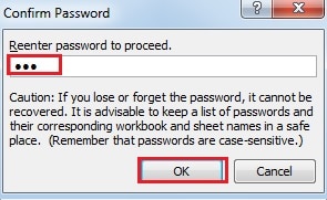
- In the “Confirm Password” window, input the password again.

- And then click “OK”.
- If you want to leave the permission in a new worksheet in case you will forget, you can check the option “Paste permission information into a new workbook”.
- And then click the button “Apply”.

- Next click “OK”.


Thus, you have finished the setting of the target cell. You can also repeat the steps to set password for the sales volume of Sophia. In addition, you can also set the two cells together. All the setting should be adjusted according your actual requirement.
- And then you can protect the worksheet with another password.
Edit Certain Range
Now you have sent the file and the corresponding password to Paul. And if John needs to modify the number, he may input the password first.
- Double click the cell.
- Then input the password into the text box.

- Next click “OK”. Thus, this cell can be edited. However, without the password of the worksheet or other range password, Paul cannot modify other cells.

Excel Disaster can Damage your Password
Even if you have set password to your Excel worksheet, it can also be damaged in a data disaster. As a result, your important data and information will leak. To avoid such accident, a third party Excel recovery tool can help you. It can get back almost all the information in your file within minutes.
Author Introduction:
Anna Ma is a data recovery expert in DataNumen, Inc., which is the world leader in data recovery technologies, including word recovery and outlook repair software products. For more information visit www.datanumen.com
Microsoft Excel предоставляет пользователю несколько, условно выражаясь, уровней защиты — от простой защиты отдельных ячеек до шифрования всего файла шифрами крипто-алгоритмов семейства RC4. Разберем их последовательно…
Уровень 0. Защита от ввода некорректных данных в ячейку
Самый простой способ. Позволяет проверять что именно пользователь вводит в определенные ячейки и не разрешает вводить недопустимые данные (например, отрицательную цену или дробное количество человек или дату октябрьской революции вместо даты заключения договора и т.п.) Чтобы задать такую проверку ввода, необходимо выделить ячейки и выбрать на вкладке Данные (Data) кнопку Проверка данных (Data Validation). В Excel 2003 и старше это можно было сделать с помощью меню Данные — Проверка (Data — Validation). На вкладке Параметры из выпадающего списка можно выбрать тип разрешенных к вводу данных:

Соседние вкладки этого окна позволяют (при желании) задать сообщения, которые будут появляться перед вводом — вкладка Сообщение для ввода (Input Message), и в случае ввода некорректной информации — вкладка Сообщение об ошибке (Error Alert):

Уровень 1. Защита ячеек листа от изменений
Мы можем полностью или выборочно запретить пользователю менять содержимое ячеек любого заданного листа. Для установки подобной защиты следуйте простому алгоритму:
- Выделите ячейки, которые не надо защищать (если таковые есть), щелкните по ним правой кнопкой мыши и выберите в контекстном меню команду Формат ячеек (Format Cells). На вкладке Защита (Protection) снимите флажок Защищаемая ячейка (Locked). Все ячейки, для которых этот флажок останется установленным, будут защищены при включении защиты листа. Все ячейки, где вы этот флаг снимете, будут доступны для редактирования несмотря на защиту. Чтобы наглядно видеть, какие ячейки будут защищены, а какие — нет, можно воспользоваться этим макросом.
- Для включения защиты текущего листа в Excel 2003 и старше — выберите в меню Сервис — Защита — Защитить лист (Tools — Protection — Protect worksheet), а в Excel 2007 и новее — нажмите кнопку Защитить лист (Protect Sheet) на вкладке Рецензирование (Reveiw). В открывшемся диалоговом окне можно задать пароль (он будет нужен, чтобы кто попало не мог снять защиту) и при помощи списка флажков настроить, при желании, исключения:

Т.е., если мы хотим оставить пользователю возможность, например, форматировать защищенные и незащищенные ячейки, необходимо установить первых три флажка. Также можно разрешить пользователям использовать сортировку, автофильтр и другие удобные средства работы с таблицами.
Уровень 2. Выборочная защита диапазонов для разных пользователей
Если предполагается, что с файлом будут работать несколько пользователей, причем каждый из них должен иметь доступ в свою область листа, то можно установить защиту листа с разными паролями на разные диапазоны ячеек.
Чтобы сделать это выберите на вкладке Рецензирование (Review) кнопку Разрешить изменение диапазонов (Allow users edit ranges). В версии Excel 2003 и старше для этого есть команда в меню Сервис — Защита — Разрешить изменение диапазонов (Tools — Protection — Allow users to change ranges):

В появившемся окне необходимо нажать кнопку Создать (New) и ввести имя диапазона, адреса ячеек, входящих в этот диапазон и пароль для доступа к этому диапазону:

Повторите эти действия для каждого из диапазонов разных пользователей, пока все они не окажутся в списке. Теперь можно нажать кнопку Защитить лист (см. предыдущий пункт) и включить защиту всего листа.
Теперь при попытке доступа к любому из защищенных диапазонов из списка, Excel будет требовать пароль именно для этого диапазона, т.е. каждый пользователь будет работать «в своем огороде».
Уровень 3. Защита листов книги
Если необходимо защититься от:
- удаления, переименования, перемещения листов в книге
- изменения закрепленных областей («шапки» и т.п.)
- нежелательных изменений структуры (сворачивание строк/столбцов при помощи кнопок группировки «плюс/минус»)
- возможности сворачивать/перемещать/изменять размеры окна книги внутри окна Excel
то вам необходима защита всех листов книги, с помощью кнопки Защитить книгу (Protect Workbook) на вкладке Рецензирование (Reveiw) или — в старых версиях Excel — через меню Сервис — Защита — Защитить книгу (Tools — Protection — Protect workbook):

Уровень 4. Шифрование файла
При необходимости, Excel предоставляет возможность зашифровать весь файл книги, используя несколько различных алгоритмов шифрования семейства RC4. Такую защиту проще всего задать при сохранении книги, т.е. выбрать команды Файл — Сохранить как (File — Save As), а затем в окне сохранения найти и развернуть выпадающий список Сервис — Общие параметры (Tools — General Options). В появившемся окне мы можем ввести два различных пароля — на открытие файла (только чтение) и на изменение:

Ссылки по теме
- Как установить/снять защиту на все листы книги сразу (надстройка PLEX)
- Подсветка незащищенных ячеек цветом
- Правильная защита листов макросом