Protect all cells in excel

Suppose that your boss wants you to protect an entire workbook, but also wants to be able to change a few cells after you enable protection on the workbook. Before you enabled password protection, you had unlocked some cells in the workbook. Now that your boss is done with the workbook, you can lock these cells.

Follow these steps to lock cells in a worksheet:

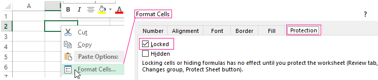
1. Select the cells you want to lock.

2. On the Home tab, in the Alignment group, click the small arrow to open the Format Cells popup window.

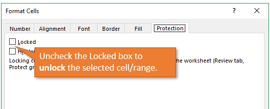
3. On the Protection tab, select the Locked check box, and then click OK to close the popup.

   Note: If you try these steps on a workbook or worksheet you haven’t protected, you’ll see the cells are already locked. This means that the cells are ready to be locked when you protect the workbook or worksheet.

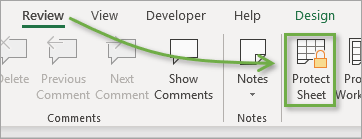
4. On the Review tab in the ribbon, in the Changes group, select either Protect Sheet or Protect Workbook, and then reapply protection. See Protect a worksheet or Protect a workbook.

   Tip: It’s a best practice to unlock any cells that you may want to change before you protect a worksheet or a workbook, but you can also unlock them after you apply protection. To remove protection, simply remove the password.

In addition to protecting workbooks and worksheets, you can also protect formulas.

Excel for the web can’t lock cells or specific areas of a worksheet.

If you want to lock cells or protect specific areas, click Open in Excel and lock cells to protect them or lock or unlock specific areas of a protected worksheet.

When it comes time to send your Excel spreadsheet, it’s important to protect the data that you’re sharing. You might want to share your data, but that doesn’t mean it should be changed by someone else.

Spreadsheets often contain essential data that shouldn’t be modified or removed by the recipient. Luckily, Excel has built-in features to protect your spreadsheets.

In this tutorial, I’ll help you make sure that your Excel workbooks maintain data integrity. Here are three key techniques you’ll learn in this tutorial:

• Password protect entire workbooks to prevent them from being opened by unauthorized users.
• Protect individual sheets and the workbook structure, to prevent the insertion or deletion of sheets in the workbook.
• Protect cells, to specifically allow or disallow changes to key cells or formulas in your Excel spreadsheets.

Even users with the best intentions may accidentally break an important or complex formula. The best thing to do is remove the option to change your spreadsheets altogether.

How to Protect Excel: Cells, Sheets, & Workbooks (Watch & Learn)

In the screencast below, you’ll see me work through several important types of protection in Excel. We’ll protect an entire workbook, a single spreadsheet, and more.

Want a step-by-step walkthrough? Check out my steps below to find out how to use these techniques. You’ll learn how to protect your workbook in Excel, as well as protecting individual worksheets, cells, and how to work with advanced settings. 

We start with broader worksheet protections, then work down to narrower targeted protections you can apply in Excel. Let’s get started learning how to protect your spreadsheet data:

1. Password Protect an Excel Workbook File

Let’s start off by protecting an entire Excel file (or workbook) with a password to prevent others from opening it.

This is a breeze to do. While working in Excel, navigate to the File tab choose the Info tab. Click on the Protect Workbook dropdown option and choose Encrypt with Password.

As is the case with any password, choose a strong and secure combination of letters, numbers, and characters, bearing in mind that passwords are case-sensitive.

It’s important to note that Microsoft has really beefed up the seriousness of their password protection in Excel. In prior versions, there were easy workarounds to bypass password protection of Excel workbooks, but not in newer versions.

In Excel 2013 and beyond, the password implementation will prevent these traditional methods to bypass it. Make sure that you store your passwords carefully and safely or you risk permanently losing access to your crucial workbooks.

Excel Workbook — Mark as Final

If you want to be a bit less forceful with your spreadsheets, consider using the Mark as Final feature. When you mark an Excel file as the final version, it switches the file to read-only mode, and the user will have to re-enable editing.

To change a file to read-only mode, return to the File > Info button, and click on Protect Workbook again. Click on Mark as Final and confirm that you want to mark the document as a final version.

Marking a file as the final version will add a soft warning to the top of the file. Anyone who opens the file after it has been marked as final will see a notice, warning them that the file is finalized. 

Marking a file as the final version is a less formal way of signaling that a file shouldn’t be changed further. The recipient still has the ability to click Edit Anyway and modify the spreadsheet. Marking a file as the final edition is more like a suggestion, but it’s a great approach if you trust the other file users.

2. Password Protect Your Excel Sheet Structure

Next up, let’s learn how to protect the structure of an Excel workbook. This option will ensure that no sheets are deleted, added, or re-arranged inside of the workbook.

If you want everyone to be able to access the workbook, but limit the changes they can make to a file, this is a great start. This protects the structure of the workbook, and limits how the user can change the sheets inside of it.

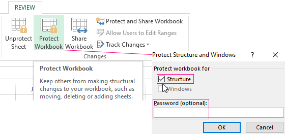
To turn on this protection, go to the Review tab on Excel’s ribbon and click on Protect Workbook.

Once this option is turned on, the following will go into effect:

• No new sheets can be added to the workbook.
• No sheets can be deleted from the workbook.
• Sheets can no longer be hidden or unhidden from the user’s view.
• The user can no longer drag and drop the sheet tabs to reorder them in the workbook.

Of course, trusted users can be given the password to unprotect the workbook and modify it. To unprotect a workbook, simply click on the Protect Workbook button again and input the password to unprotect the Excel workbook.

3. How to Protect Cells in Excel

Now, let’s get down to really detailed methods for protecting a spreadsheet. So far, we’ve been password protecting an entire workbook or the structure of an Excel file. In this section, we dig into how to protect your cells in Excel with specific settings you can apply. We cover how to allow or block certain types of changes to be made to parts of your spreadsheet.

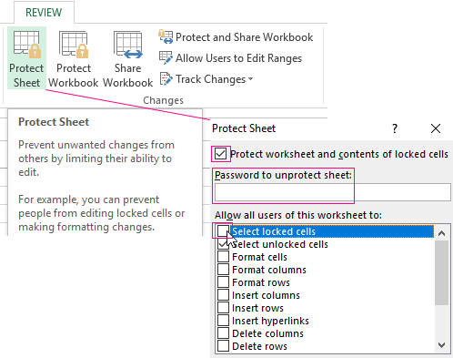
To get started, find Excel’s Review tab, and click on Protect Sheet. On the pop-up window, you’ll see a huge set of options. This window allows you to fine-tune how you want to protect the cells in your Excel spreadsheet. For now, let’s leave the settings at their default.

This option allows for very specific protections of your spreadsheet. By default, the options will almost totally lock down the spreadsheet. Let’s add a password so that the sheet is protected. If you press OK at this point, let’s see what happens when you attempt to change a cell.

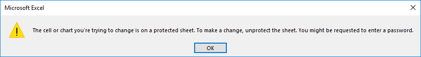
Excel throws off an error that the cell is protected, which is exactly what we wanted.

Basically, this option is crucial if you want to ensure that your spreadsheet isn’t changed by others who have access to the file. Using the protect sheet feature is a way that you can selectively protect the spreadsheet.

To unprotect the sheet, simply click on the Protect Sheet button and re-enter the password to remove the protections added to the sheet.

Specific Protections in Excel

Let’s take a second look at the options that show when you start to protect a sheet in Excel workbooks.

The Protect Sheet menu lets you refine the options for sheet protection. Each of the boxes on this menu lets the user change slightly more inside of a protected worksheet.

To remove a protection, check the respective box in the list. For example, you could allow the spreadsheet user to Format cells by checking the corresponding box.

Here are two ideas on how you could selectively allow the user to change the spreadsheet:

• Check the Format cells, columns, and rows boxes to let the user change the visual appearance of cells without modifying the original data.
• Insert columns and rows could be checked so that the user can add more data, while protecting the original cells.

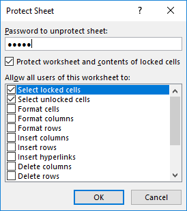
The important box to leave checked is the Protect worksheet and contents of locked cells box. This protects the data inside of cells. 

When you’re working with crucial financial data or formulas that will be used in making decisions, you have to maintain control of the data and ensure that it doesn’t change. Using these types of targeted protections is an important Excel skill to master.

Recap and Keep Learning More About Excel

Locking up a spreadsheet before you send it is crucial to protecting your valuable data and making sure that it’s not misused. The tips I shared in this tutorial help you maintain control of that data even after your Excel spreadsheet is forwarded and shared.

All of these tips are additional tools and steps to becoming an advanced Excel user. Protecting your workbooks is a specific skill, but there are lots of ways to improve your performance. As always, there’s room to grow your Excel skills further. Here are some helpful Excel tutorials with important skills to master next:

• PivotTables are a great tool for working with spreadsheet data. Here’s 5 Advanced Excel Pivot Table Techniques to learn now.
• ExcelZoo has a listing of additional tutorials for protecting your workbooks, sheets, and cells.
• Condition formatting changes how a cell looks based on what’s inside of it. Here’s a comprehensive Excel tutorial on How to Use Conditional Formatting.

How do you protect your important business data when sharing it? Let me know in the comments section if you use these protection tools or others I may not know about.

Did you find this post useful?

I believe that life is too short to do just one thing. In college, I studied Accounting and Finance but continue to scratch my creative itch with my work for Envato Tuts+ and other clients. By day, I enjoy my career in corporate finance, using data and analysis to make decisions.

I cover a variety of topics for Tuts+, including photo editing software like Adobe Lightroom, PowerPoint, Keynote, and more. What I enjoy most is teaching people to use software to solve everyday problems, excel in their career, and complete work efficiently. Feel free to reach out to me on my website.

Data in Excel can be protected from extraneous interference. This is important, because sometimes you spend a lot of time and effort creating a pivot table or a large array, and another person accidentally or intentionally changes or completely deletes all your work.

Let’s consider the ways of protecting an Excel document and its single elements.



Protection of Excel cells from changing

How to put protection on a cell in Excel? By default, all cells in Excel are protected (locked). It’s easy to check: right-click on any cell, select «Format Cells» – «Protection». We can see that the check box on the «Locked» item is selected. But this does not mean that they are protected from changes.

Why do we need this information? The thing is that Excel doesn’t provide the function allowing you to protect a single cell. We can enable protection of the worksheet, and then all the cells on it will be protected from editing and other interference. On the one hand, it is convenient, but what if we don’t need to protect all the cells, but only some of them?

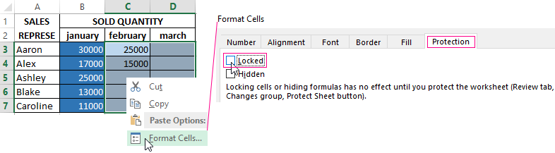
Let’s consider an example. We have a simple spreadsheet with data. We need to send this spreadsheet to branch stores, so that the stores could fill in the «SOLD QUANTITY» column and send it back. To avoid making any changes to other cells, let’s protect them.

First, remove protection from those cells to which employees of branch stores will make changes. Select C3: D7, right-click to open the menu, select «Format Cells» and remove the check box from «Locked».

Now select «REVIEW» – «Changes» — «Protect Sheet» tab. A window appears with 2 check boxes selected. Clear the first one, to exclude any interference of branch stores’ employees, except for filling «SOLD QUANTITY» column. Come up with a password and click OK.

Warning! Do not forget your password!

Now other people can only enter some value in C3: D7 range. Since we have limited all other actions, no one can even change the background color. All the formatting tools on the top toolbar aren’t active, that is, they do not work.



Protection of an Excel workbook from editing

If several people work on one computer, it is advisable to protect their documents from editing by third parties. It is possible to put protection not only on separate worksheets, but also on the whole workbook.

When the workbook is protected, outsiders can open the document, see the written data, but they cannot rename the sheets, insert a new one, change their location, etc. Let’s have a try.

Save the previous formatting. That is, you still can make changes only in «SOLD QUANTITY» column. To protect the workbook completely, select «REVIEW» – «Changes» — «Protect Workbook» tab. Click the check box opposite «Structure» item and come up with a password.

Now, if we try to rename the worksheet, we will not succeed. All commands are gray-colored: they don’t work.

The protection from the worksheet and the workbook is removed with the same buttons. When removing, the system will require the same password.

Whether you are trying to steer clear of accidental overwrites, feeling fickle, or trying to protect some important data; all your reasons are good enough to lock cells in Excel. Locking a cell means that the contents of the cell cannot be changed and the user will receive a prompt when trying to edit a locked cell, not allowing edits to the locked cell.

Some fun facts about cell locking:

• All cells are locked by default (but not protected).
• The cells only get their locked properties when the sheet is protected.
• Once the cells are locked and the sheet protected, the locked cells cannot be edited.
• When trying to edit a locked cell, a prompt will appear, hampering the edit.

There’s a whole world of cell locking but also of cell unlocking. This tutorial will give you the 101 on locking cells, formulas, sheets, and more with locking’s sidekick; unlocking.

How to Lock Cells in Excel

All the cells in a workbook are locked by default. Great, so why are we here? Because these locked cells need to be protected in order for them to work as expected.

You can think of it as – Lock is a kind of flag associated with each cell that enables Excel to understand if that particular cell should or shouldn’t be allowed for editing when sheet protection is turned on. Without the sheet protection feature turned on both locked as well as unlocked cells behave the same way.

For you to lock cells in a way that their contents cannot be altered by other users, the cells need a double treatment:

• Step 1 – The cells have to be locked and
• Step 2 – The sheet has to be protected.

A little heads up. Whether locking a cell, a range of cells, formulas in cells, a column; essentially all of this is «cell» locking and requires relevant selection of the cells. Now let’s find out more about the mentioned double treatment; locking and protecting.

How to Lock all the Cells in a Worksheet

Let’s try to understand how to lock all the cells in a worksheet.

Step 1 – All Cells Need to be Locked

The first part of the double treatment for all the cells is already automatically done; since all the cells are locked by default in Excel. So, we can directly move to Step 2. In Step 2, the sheet protection feature needs to be activated. Let’s see how to get it done.

Step 2 – Protecting the Worksheet

Time to protect the worksheet.

• In the Review tab, from the Protect section, click the Protect Sheet.

• Clicking this button will have a Protect Sheet dialog box appear as shown below.

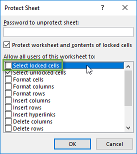
• The first text box is for setting a password on the sheet which needs to be entered when trying to unprotect the sheet. This is optional and can be skipped. The ‘Protect worksheet and contents of locked cells’ tick box should be automatically checked. Leave it checked. Under Allow all users of this worksheet to: select how much control you would like to provide the users by checking the tick boxes against the relevant options and click OK.

• If you used a password, you would see a dialog box asking to reconfirm the password. If you haven’t specified a password, your sheet should be protected now. Nearly all of the options on the ribbon should be disabled.

• Trying to change any cell on the worksheet will not work, and a window hindering the attempted changes will pop up.

How to Lock Specific Cells in a Worksheet

Interestingly, locking specific cells has a few additional steps than locking all of the cells. We will go back to assuming the initial state of a workbook i.e. when all cells are locked by default and the worksheet is unprotected. We need to unlock all the cells and then lock the chosen cells. Here are the steps to do this:

The cells with the values in the blue-colored font are the 2 cells we want to lock on the sheet so that their values cannot be changed. Apart from these two, we wish to lock and protect all the other cells on the sheet.

Step 1 – Unlock all Cells on the Worksheet

So, the prerequisite here is to unlock all the cells on the worksheet. To do this follow along.

• Select all the cells on the sheet and navigate to the ‘Home’ tab, in the ‘Alignment’ section, click the ‘Alignment Settings’ option (the little diagonally pointing arrow in the bottom right corner).

• This will open the Format Cells dialog box. In the Format Cells dialog box, select the Protection tab. The Locked checkbox will be checked by default. Uncheck it to unlock all the cells on the worksheet.

• Click OK and all the cells in the current worksheet will be unlocked.

Step 2 – Lock Specific Cells on the Worksheet

Now we will select the cells on the sheet that we want to lock i.e., D10 and E11. To lock these cells follow the below steps:

• Select the D10 and E11 cells, we will again launch the Format Cells dialog box to lock the chosen cells. Click the ‘Alignment Settings’ option in the Alignment section under the Home.

• In the Format Cells dialog box, select the Protection tab. Check the Locked tick box to lock the chosen cells.

Step 3 – Protecting the Worksheet

Now we have locked the chosen cells. If you try, you will notice that you can still edit the locked cells. For cell locking to work the worksheet needs to be protected and this is what we are going to do now.

• Under the Review tab, in the Protect section, click the Protect Sheet. This will launch the Protect Sheet dialog box.

• Add a password if you wish (optional). Check if the Protect worksheet and contents of locked cells tick box is automatically checked. Leave it checked. Under Allow all users of this worksheet to: select how much control you would like to provide the users by checking the tick boxes against the relevant options and click OK.
• Reconfirm the password if any, is used.

Now you can check the sheet; only meddling with the locked cells will trigger the sheet protection prompt. The other cells are still editable.

Recommended Reading: All About Page Breaks in Excel

How to Lock all Formula Cells in a Worksheet

To protect formulas in a sheet, you need to unlock all the cells in the sheet, select the formula cells, lock them and then protect the sheet. Pretty much like how we lock specific cells (mentioned above). For big and complex worksheets, this would surely be a very daunting task with so many formula cells to lock. Not to worry, we will have Excel select the formula cells itself, which we will then lock and protect the sheet.

Easy now, right? Let’s see the steps for this:

Step 1 – Unlock all Cells on the Worksheet

So, the prerequisite here is to unlock all the cells on the worksheet. To do this follow along.

• Select all the cells on the sheet and navigate to the ‘Home’ tab, in the ‘Alignment’ section, click the ‘Alignment Settings’ option (the little diagonally pointing arrow in the bottom right corner).

• This will open the Format Cells dialog box. In the Format Cells dialog box, select the Protection tab. The Locked checkbox will be checked by default. Uncheck it to unlock all the cells on the worksheet.

• Click OK and all the cells in the current worksheet will be unlocked.

Step 2 – Find and Lock Cells Containing Formulas

Now, let’s quickly try to find and lock the cells that contain formulas:

• Under the Home tab, from the Editing section, click on the Find & Select button, then click on the Go To Special. This will open the Go To Special window.

• In the Go To Special dialog box, select Formulas from the radio buttons. All the checkboxes boxes under the Formulas radio button should get automatically checked.

• Click OK and all the formula cells on the worksheet will be selected now. Be careful not to click any other cell on the worksheet as that will unselect the formula cells.
• After selecting the cells, we will again launch the Format Cells window to lock the chosen cells. Click the ‘Alignment Settings’ option in the Alignment section under the Home.

• In the Format Cells dialog box, select the Protection Check the Locked tick box to lock the chosen cells.

This has locked the chosen cells. If you try, you will notice that you can still edit the locked cells. The sheet needs to be protected for the cell locking to work.

Pro Tip: If you want your formulas to be hidden and not displayed in the formula bar after locking the cells, click the Hidden checkbox on the Format cells window.

Step 3 – Protecting the Worksheet

Now we have locked the chosen cells. If you try, you will notice that you can still edit the locked cells. For cell locking to work, the worksheet needs to be protected and this is what we are going to do now.

• Under the Review tab, in the Protect section, click the Protect Sheet. This will launch the Protect Sheet dialog box.

• Add a password if you wish (optional). Check if the Protect worksheet and contents of locked cells tick box is automatically checked. Leave it checked. Under Allow all users of this worksheet to: select how much control you would like to provide the users by checking the tick boxes against the relevant options and click OK.
• Reconfirm the password if any is used.

If you check now, the entire worksheet can be edited except the cells with the formulas.

How to Lock a Column in a Worksheet

Locking a column works on pretty much the same principle – unlock all the cells in the sheet, select all the cells in the column(s) you wish to lock, lock the cells, protect the sheet.

Here are the detailed steps:

Step 1 – Unlock all Cells on the Worksheet

So, the prerequisite here is to unlock all the cells on the worksheet. To do this follow along.

• Select all the cells on the sheet and navigate to the ‘Home’ tab, in the ‘Alignment’ section, click the ‘Alignment Settings’ option (the little diagonally pointing arrow in the bottom right corner).

• This will open the Format Cells dialog box. In the Format Cells dialog box, select the Protection tab. The Locked checkbox will be checked by default. Uncheck it to unlock all the cells on the worksheet.

• Click OK and all the cells in the current worksheet will be unlocked.

Step 2 – Select & Lock all the Column Cells

Since all the cells in the worksheet are unlocked now, so we will now try to select the column that we want to lock and set the Locked property to true for all its cells.

• Select the column(s) you want to lock. For our case, we want to lock the prices so we’ll select column C by clicking on C. You can also select multiple columns.

• After selecting the column, we will again launch the Format Cells dialog box to lock the chosen column. Click the Alignment Settings Option in the Alignment section under the Home.

• In the Format Cells dialog box, select the Protection Check the Locked tick box to lock the chosen column.

This has locked the chosen column. If you try, you will notice that you can still edit the cells in the locked column. In order for the locking to work, the sheet needs to be protected.

Step 3 – Protecting the Worksheet

To protect the sheet:

• Under the Review tab, in the Protect section, click the Protect Sheet This will launch the Protect Sheet dialog box.

• Add a password if you wish (optional). Check if the Protect worksheet and contents of locked cells tick box is automatically checked. Leave it checked. Under Allow all users of this worksheet to: select how much control you would like to provide the users by checking the tick boxes against the relevant options and click OK.
• Reconfirm the password if any is used.

In this way, the entire column cannot be edited and gets locked.

How to Lock an Entire Workbook

Now that you know how to protect sheets, you may have noticed a button right next to Protect Sheet which is for protecting the whole workbook. Protecting a workbook doesn’t allow users to make changes to the structure of the workbook. For example – users will not be able to add, move, rename or delete sheets in a workbook. However, they can edit and delete the cells unless the cells are locked and worksheet protection is turned on.

To lock a workbook follow these steps:

• Under the Review tab, in the Protect section, click the button Protect Workbook.

• This will launch the Protect Structure and Windows dialog. On this dialog box make sure the Structure tick box is checked. Adding the password is optional. Add password in the Password box if you wish.

• Once done, click OK. It will prompt you to re-enter the password if you have added one, re-enter the password and we are done.

Your entire workbook is now protected. Workbook protection can be verified in three ways:

• The highlighted Protect Workbook button as shown below.

• The inaccessibility of many options (like insert, delete, rename, etc) on the sheet tab right-click menu as shown below.

• The Protect Workbook confirmation on the info page of the file. To check this, navigate to the File tab, then the Info tab to view this.

How To Unlock Specific Cells Ranges in a Worksheet

If you wish to lock specific cells in a sheet, it’s equally possible to want to unlock specific cells in a protected sheet for users to be able to change just a certain range of cells. We will use the Allow Edit Ranges feature to unlock some chosen range of cells. If you find yourself unable to use the feature, unprotect the sheet to make it available.

Without a password, Allow Edit Ranges feature works similar to the selective locking procedure that we have seen above (Unlock all cells, Lock specific cells and then Protect the worksheet). But the real difference can be seen when we use a range editing password.

With a range editing password, the cell ranges that we mark editable only become editable after the password is entered. It should be noted that the range editing password can be (should be) very different from the sheet protection password.

The benefit of this can be clearly seen with an example –

Suppose you have a spreadsheet that needs to be shared with multiple teams in your project. Now, you want that only one team should be able to edit a preset range of cells from the sheet. While all the other teams should just be able to use the spreadsheet in protected form. So, in this case, you can easily protect the worksheet allowing the specific range to be editable with a password using this feature. And share the password only with the team that needs to make the changes.

In this way, anyone who has the range editing password would be able to edit the editable range in the worksheet. While for others the entire worksheet will be locked. So, this just adds a layer of protection over the sheet protection feature of Excel.

Now let’s come back to our example and understand how to make use of this feature. The cells we would want to keep unlocked are D3:D7 to be able to edit the quantities. Follow along –

• Select the cells you would want to keep unlocked.

• Next, in the Review tab, in the Protect section, click Allow Edit Ranges option. The Allow Users to Edit Ranges dialog box will appear.

• Click New. In the New Range dialog box, Excel has already provided the title (changing it is optional) and the selected cell references (the range that we want to keep unlocked). Add the range editing password and click OK.

• Reenter the password to confirm it. Click OK.

• After the range editing password is set, click the Protect Sheet button and protect the sheet with or without a password. And we are done

Trying to change any locked cell on the worksheet will not work and a window hindering the attempted changes will pop up.

Upon trying to edit any cells from D3:D7, you will receive a prompt demanding the password to unlock the cells. Type the password to unlock the cells.

How to Unprotect Sheets in Excel

Let’s talk about unprotecting worksheets. To talk about this feature let’s assume we are working on a sheet that is protected and all the cells are locked for editing.

Follow along  to unprotect and unlock the cells:

• The only thing that we need to do is – to Unprotect the sheet. To do this navigate to the Review tab and click the Unprotect Sheet button. The Unprotect Sheet button will only be available on the ribbon if the sheet is already protected.

• If the sheet was locked without a password it would get unlocked right away. However, Excel will ask you to enter the password if the sheet was locked with a password.
• After the sheet protection is turned off all the cells on the sheet should become editable.

How to Find/Format Locked and Unlocked Cells

After knocking into locked cells over and over while trying to edit them and being unable, we need to get this straight. Let’s find out on the face of it, which cells are unlocked and which aren’t. If you’re feeling a tad impatient, a speedy way to look locked and unlocked cells up is through the CELL function which will display locked cells as 1 (1 means TRUE) and unlocked as 0 (0 means FALSE).

See the formula:

=CELL("protect",C3)

C3 refers to the cell you want to check for its locked or unlocked status. In our sheet, we have locked the cells E3:E7. Here is what our sheet looks like after applying the CELL function:

For a small sheet, this is quite alright but we assure you there’s a better way than having your eyes sift through 1’s and 0’s. We will still use the CELL function but we will use it with the Conditional Formatting feature. Here we have the steps:

• Select all the cells on the worksheet.
• Go to Home > Styles section > Conditional Formatting button > New Rule.

• In the Formatting Rule dialog box. Select Use a formula to determine which cells to format.

• Enter the following formula and set the format you want for the locked cells by clicking on the Format (We will select gray color fill).

=CELL("protect", A1) = 1

• Click OK.

Our locked cells E3:E7 have been conditionally formatted and we can easily identify them based on the background fill.

Prevent Locked Cells from Being Selected

Instead of the users trying to edit a locked cell, receiving the locked cell prompt, clicking OK, and then moving onto what they should do, you can save their time (and yours) by preventing locked cells from being selected in the first place.

You select a cell by clicking on it with the mouse or by navigating to it with the keyboard. All you need to do to prevent locked cells from being selected is unchecking the Select locked cells tick box in the sheet protection dialog box.

• In the Review tab, from the Protection section, click the Protect Sheet button.
• Uncheck the Select locked cells tick box from the Protect Sheet dialog box as shown.

• Click OK.

Now the locked cells cannot be selected by any means. If you try to click a locked cell, no selection on the cell will be made and the selection will remain on any previously selected cell. If you try to navigate to it, the locked cell will be skipped and the nearest editable cell will be selected.

Hide Formulas In Locked Cells

The formula in a cell can be viewed in the Formula bar when that cell is selected, no matter if the cell is locked or unlocked. If you’re feeling secretive and do not want one or more formulas to show in locked cells, we can achieve it in a couple of ways.

You can either prevent the selection of the locked cells with the formulas (mentioned above). If the cell won’t be selected, you can’t view the formula. Or we can hide the formulas. This can be done to already locked cells or the cells can be locked and the formulas can be hidden together. You only have to check the Hidden tick box while locking cells. The steps are as follows:

Step 1 – Mark the Cells Locked and Hidden

• Select the cells containing the formulas you want to hide and also lock. In our case, we are going to lock and hide the formulas of E3:E7.
• After selecting the desired cells, we will launch the Format Cells dialog box to lock the chosen column. Click the Alignment Settings Option in the Alignment section under the Home.

• In the Format Cells dialog box, make sure to check both the tick boxes; Locked and Hidden.

Step 2: Protecting the Worksheet

To protect the sheet:

• Under the Review tab, in the Protect section, click the Protect Sheet This will launch the Protect Sheet dialog box.

• Add a password if you wish (optional). Check if the Protect worksheet and contents of locked cells tick box is automatically checked. Leave it checked. Under Allow all users of this worksheet to: select how much control you would like to provide the users by checking the tick boxes against the relevant options and click OK.
• Reconfirm the password if any is used.

And we are done! If you select the locked cells now, you can’t see the formula in the formula bar. The selection of these cells doesn’t display anything in the formula bar, not even the value itself.

Recommended Reading: Lock & Hide Formulas in Excel – 2 Easy Ways

And that’s that! We hope to have given you some command over cell locking and protection. While you and the sheets are sworn to secrecy, we’ll prepare some more Excel-ling for you; «locked» and loaded.

Bottom Line: Learn how to lock individual cells or ranges in Excel so that users cannot change the formulas or contents of protected cells. Plus a few bonus tips to save time with the setup.

Skill Level: Beginner

Video Tutorial

Download the Excel File

You can download the file that I use in the video tutorial by clicking below.

Protecting Your Work from Unwanted Changes

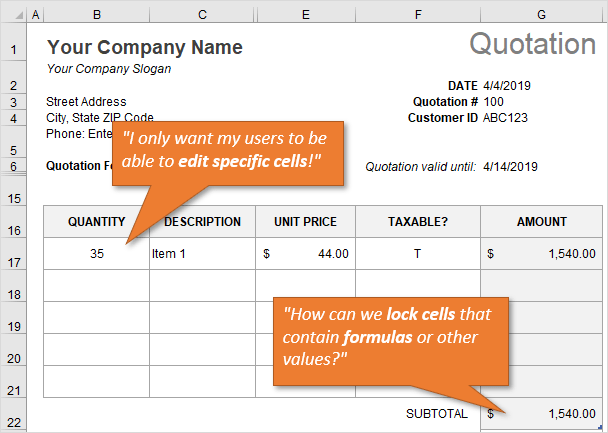
If you share your spreadsheets with other users, you’ve probably found that there are specific cells you don’t want them to modify. This is especially true for cells that contain formulas and special formatting.

The great news is that you can lock or unlock any cell, or a whole range of cells, to keep your work protected. It’s easy to do, and it involves two basic steps:

1. Locking/unlocking the cells.
2. Protecting the worksheet.

Here’s how to prevent users from changing some cells.

Step 1: Lock and Unlock Specific Cells or Ranges

Right-click on the cell or range you want to change, and choose Format Cells from the menu that appears.

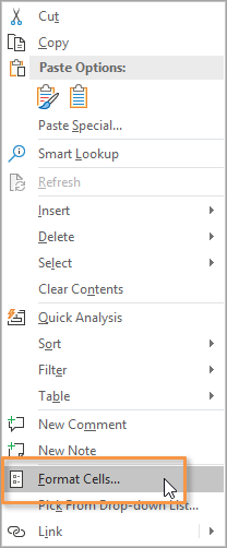
This will bring up the Format Cells window (keyboard shortcut for this window is Ctrl + 1.). Choose the tab that says Protection.

Next, make sure that the Locked option is checked.

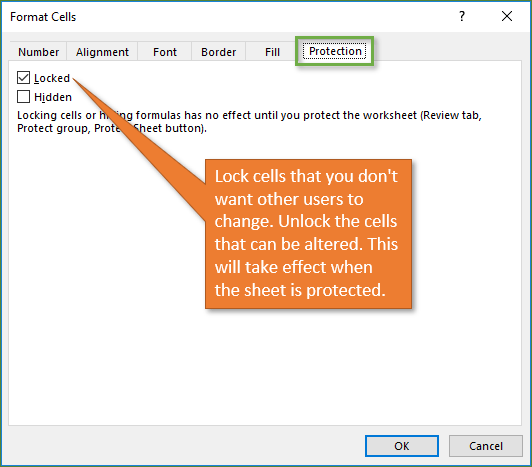
Locked is the default setting for all cells in a new worksheet/workbook.

Once we protect the worksheet (in the next step) those locked cells will not be able to be altered by users.

If you want users to be able to edit a particular cell or range, uncheck the Locked box so they are unlocked. Since cells are locked by default, most of the job will be going through the sheet and unlocking cells that can be edited by users.

I share some shortcuts to make this process faster in the Bonus section below.

Step 2: Protect the Worksheet

Now that you’ve locked/unlocked the cells that you want users to be able to edit, you want to protect the sheet. Once you protect the sheet, users cannot change the locked cells. However, they can still modify the unlocked cells.

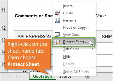
To protect the sheet, simply right-click on the tab at the bottom of the sheet, and choose Protect Sheet… from the menu.

This will bring up the Protect Sheet window. If you want your sheet to be password protected, you have the option of entering a password here. Adding a password is optional. Click OK.

If you’ve chosen to enter a password, then you will be prompted to verify your entry after you’ve clicked OK.

With the sheet protected, users will be unable to change the cells that are locked. If they try to make changes, they will get an error/warning message that looks like this.

You can unprotect the sheet in the same way that you protected it, by right-clicking on the sheet tab. An alternative way to protect and unprotect sheets is by using the Protect Sheet button in the Review tab of the Ribbon.

The button text displays the opposite of the current state. It says Protect Sheet when the sheet is unprotected, and Unprotect Sheet when it is protected.

It’s important to note that all cells can be edited when the sheet is unprotected. After making changes you must protect the sheet again and Save the workbook before sending or sharing with other users.

3 Bonus Tips for Locking Cells and Protecting Sheets

As you can see, it is fairly simple to protect your formulas and formatting from being changed! But I’d like to leave you with three tips to help make it faster & easier for both you and your users.

1. Prevent Locked Cells From Being Selected

This tip will help make it faster and easier for your users to input data in the sheet.

Turning off the Select locked cells option prevents the locked cells from being selected with either the mouse or keyboard (arrow or tab keys). This means users will only be able to select the unlocked cells that they need to edit. They can quickly hit the Tab, Enter, or arrow keys to move to the next editable cell.

To make this change, you just uncheck the option that says “Select locked cells” on the Protect Sheet window.

After pressing OK, you will only be able to select the unlocked cells.

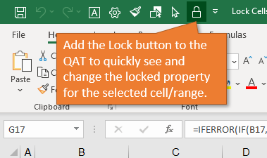
2. Add a button for locking cells to the Quick Access Toolbar

This allows you to quickly see the locked setting for a cell or range.

From the Home tab on the Ribbon, you can open the drop-down menu under the Format button and see the option to Lock Cell.

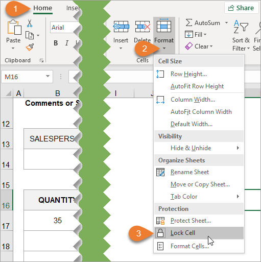
If you right-click on the Lock Cell option, another menu appears giving you the option to add the button to the Quick Access Toolbar.

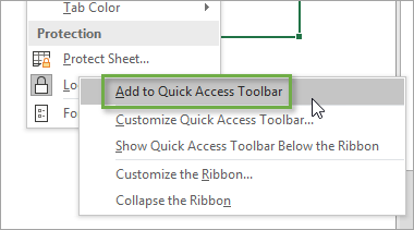
When you select this option, the button will be added to the Quick Access Toolbar at the top of the workbook. This button will remain each time you use Excel. You can easily lock and unlock specific cells on your sheet by clicking on this button.

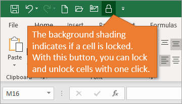
You can also see if the active cell locked or unlocked. The button will have a dark background if the selection is locked.

It’s important to note that this only shows the locked state of the active cell. If you have multiple cells selected, the active cell is the cell you selected first and appears with no fill shading.

Mixed Lock State

If you select a range that contains both locked and unlocked cells, you will see a solid box for the Locked checkbox in the Format Cells window. This denotes the mixed state.

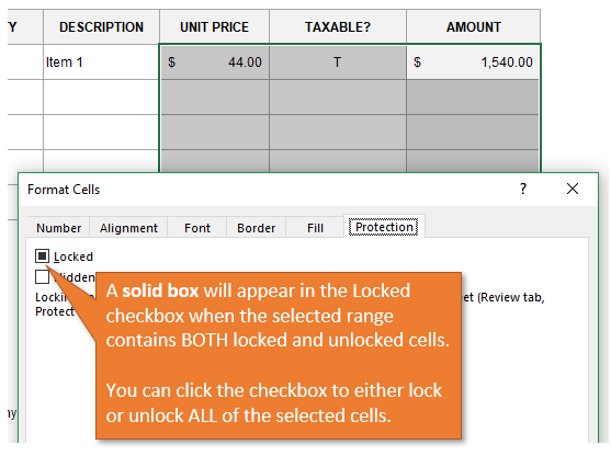
You can click the checkbox to lock or unlock ALL cells in the selected range.

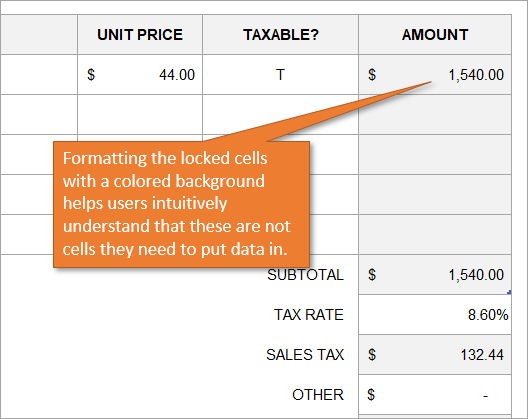
3. Use different formatting for locked cells

By changing the formatting of cells that are locked, you give your users a visual clue that those cells are off limits. In this example the locked cells have a gray fill color. The unlocked (editable) cells are white. You can also provide a guide on the sheet or instructions tab.

You might be wondering where I found this template for a quote. I got it from the template library. You can access the library by going to the File tab, choosing New, and using the search word “quote.”

You can find all sorts of useful templates there, including invoices, calendars, to-do lists, budgets, and more.

Conclusion

By locking your cells and protecting your sheet, you can keep your formulas safe from tampering by other users, and prevent mistakes.

I hope this simple tutorial proves helpful to you. Please leave a comment below if you have any tips or questions about locking cells, protecting sheets with passwords, or preventing users from changing cells.

Thank you! 🙂