
Excel for Microsoft 365 Excel for Microsoft 365 for Mac Excel for the web Excel 2021 Excel 2021 for Mac Excel 2019 Excel 2019 for Mac Excel 2016 Excel 2016 for Mac Excel 2013 Excel 2010 Excel 2007 Excel for Mac 2011 Excel Starter 2010 More…Less
This article describes the formula syntax and usage of the PRODUCT function in Microsoft Excel.
Description
The PRODUCT function multiplies all the numbers given as arguments and returns the product. For example, if cells A1 and A2 contain numbers, you can use the formula =PRODUCT(A1, A2) to multiply those two numbers together. You can also perform the same operation by using the multiply (*) mathematical operator; for example, =A1 * A2.
The PRODUCT function is useful when you need to multiply many cells together. For example, the formula =PRODUCT(A1:A3, C1:C3) is equivalent to =A1 * A2 * A3 * C1 * C2 * C3.
Syntax
PRODUCT(number1, [number2], …)
The PRODUCT function syntax has the following arguments:
-
number1 Required. The first number or range that you want to multiply.
-
number2, … Optional. Additional numbers or ranges that you want to multiply, up to a maximum of 255 arguments.
Note: If an argument is an array or reference, only numbers in the array or reference are multiplied. Empty cells, logical values, and text in the array or reference are ignored.
Example
Copy the example data in the following table, and paste it in cell A1 of a new Excel worksheet. For formulas to show results, select them, press F2, and then press Enter. If you need to, you can adjust the column widths to see all the data.
|
Data |
||
|
5 |
||
|
15 |
||
|
30 |
||
|
Formula |
Description |
Result |
|
=PRODUCT(A2:A4) |
Multiplies the numbers in cells A2 through A4. |
2250 |
|
=PRODUCT(A2:A4, 2) |
Multiplies the numbers in cells A2 through A4, and then multiplies that result by 2. |
4500 |
|
=A2*A3*A4 |
Multiplies the numbers in cells A2 through A4 by using mathematical operators instead of the PRODUCT function. |
2250 |
Need more help?
Продукт в Excel
Функция Product excel — это встроенная математическая функция, которая используется для вычисления произведения или умножения данного числа, предоставленного этой функции в качестве аргументов, например, если мы предоставим аргументы этой формулы как 2 и 3 как = PRODUCT (2,3) тогда отображается результат 6, эта функция умножает все аргументы.
Функция произведения в excel принимает аргументы (вводятся как числа) и выдает произведение (умножение) в качестве вывода. Если ячейки A2 и A3 содержат числа, то мы можем умножить эти числа с помощью ПРОДУКТА в Excel.
Формула ПРОДУКТА в Excel
= ПРОДУКТ (число1, [число2], [число3], [число4],….)
Объяснение
Формула ПРОДУКТА в Excel имеет как минимум один аргумент, а все остальные аргументы являются необязательными. Всякий раз, когда мы передаем одно входное число, оно возвращает значение как 1 * число, то есть само число. ПРОДУКТ в Excel относится к категории математических / тригонометрических функций. Эта формула ПРОДУКТА в Excel может принимать до 255 аргументов в более поздней версии после Excel 2003. В Excel версии 2003 аргумент был ограничен до 30 аргументов.
Формула ПРОДУКТА в Excel не только принимает в качестве аргумента введенный номер один за другим, но также может принимать диапазон и возвращать продукт. Итак, если у нас есть диапазон значений с числами и нам нужен их продукт, мы можем сделать это либо умножением каждого из них, либо напрямую с помощью формулы ПРОДУКТ в Excel, минуя диапазон значений.
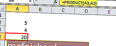
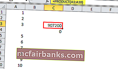
На приведенном выше рисунке мы хотим умножить все значения вместе, указанные в диапазоне A1: A10, если мы сделаем это с помощью математического оператора multiply (*), потребуется много времени по сравнению с достижением того же самого с помощью функции PRODUCT в excel. так как нам нужно будет выбрать каждое значение и умножить, тогда как, используя продукт в excel, мы можем передать значения напрямую как диапазон, и он даст результат.
= ПРОДУКТ (A1: A10)
Следовательно, формула ПРОДУКТ в Excel = ПРОДУКТ (A1: A10) эквивалентна формуле = A1 * A2 * A3 * A4 * A5 * A6 * A7 * A8 * A9 * A10
Однако единственное отличие состоит в том, что когда мы используем функцию ПРОДУКТ в Excel и если мы оставили ячейку пустой, ПРОДУКТ в Excel принимает пустую ячейку со значением 1, но с помощью оператора умножения, если мы оставили ячейку пустой, Excel примет значение равно 0, и результат будет 0.
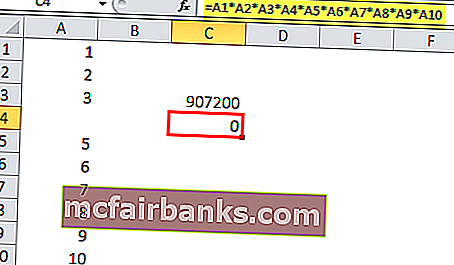
Когда мы удалили значение ячейки A4, excel считает его 0 и возвращает результат 0, как показано выше. Но когда мы использовали функцию ПРОДУКТ в excel, он взял диапазон ввода A1: A10, кажется, что ПРОДУКТ в excel игнорирует ячейку A4, которая была пустой, однако он не игнорирует значение пустой ячейки, а берет пустое ячейка со значением 1. Он принимает диапазон A1: A10, рассматривает A4 со значением 1 и умножает значения ячеек вместе. Он также игнорирует текстовые значения и логические значения. В продукте Excel даты и числовые значения рассматриваются как числа. Каждый аргумент может быть предоставлен как отдельное значение или ссылка на ячейку или как массив значений или ячеек.
Для небольших математических вычислений мы можем использовать оператор умножения, но в случае, если нам нужно иметь дело с большим набором данных, в котором задействовано умножение нескольких значений, эта функция ПРОДУКТ служит большой цели.
Итак, функция ПРОИЗВОДИТ в Excel полезна, когда нам нужно умножить множество чисел, заданных в диапазоне.
Примеры
Давайте посмотрим ниже на некоторые примеры функции ПРОДУКТ в Excel. Эти примеры функций ПРОДУКТ в Excel помогут вам изучить использование функции ПРОДУКТ в Excel.
Вы можете скачать этот шаблон Excel для функции PRODUCT здесь — Шаблон для функции PRODUCT Excel
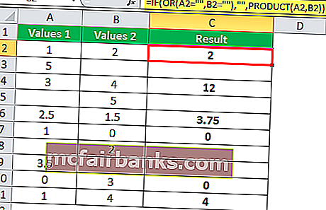
Пример # 1
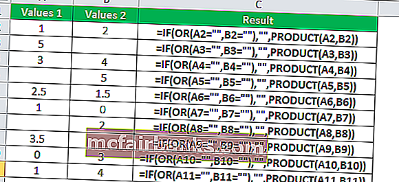
Предположим, у нас есть набор значений в столбцах A и B, который содержит числовые значения с некоторыми пустыми ячейками, и мы хотим умножить каждое значение столбца A на столбец B таким образом, чтобы если какая-либо из ячеек содержала пустое значение, мы получить пустое значение иначе возвращает произведение двух значений.
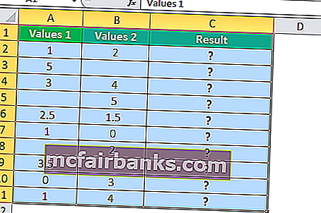
Например, ячейка B2 пуста, поэтому результатом должно быть пустое значение в ячейке C2. Таким образом, мы будем использовать условие ЕСЛИ вместе с функцией ИЛИ. Если одно из значений ячейки ничего не возвращает, ничто другое не возвращает произведение чисел.
Итак, формула ПРОДУКТА в Excel, которую мы будем использовать,
= ЕСЛИ (ИЛИ (A2 = ””, B2 = ””), ””, ПРОИЗВОД (A2, B2))
Применяя формулу ПРОДУКТА в Excel к каждой ячейке, которую мы имеем
Выход:
Пример # 2 — Вложение функции продукта
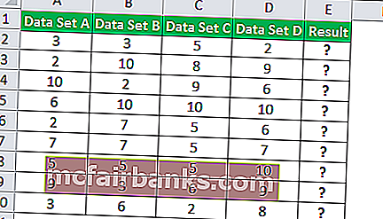
Когда ПРОДУКТ в Excel используется внутри другой функции в качестве аргумента, это называется вложением функции ПРОДУКТ в Excel. Мы можем использовать другие функции и передавать их в качестве аргумента. Например, предположим, что у нас есть четыре набора данных в столбцах A, B, C и D. Нам нужно произведение значения суммы из первого набора данных и второго набора данных на сумму значений из третьего и четвертого наборов данных.
Итак, мы будем использовать функцию SUM и передадим ее в качестве аргумента функции PRODUCT в excel. Нам нужно произведение суммы значений набора данных A и набора данных B, которая равна 3 + 3, умноженная на сумму значений набора данных C и C, которая равна (5 + 2), поэтому результат будет (3 + 3 ) * (5 + 2).
= ПРОДУКТ (СУММ (A2: B2); СУММ (C2: D2))
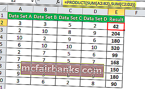
В приведенном выше примере функция суммы передается в качестве аргумента функции ПРОДУКТ в Excel, это называется вложением. Мы можем даже другие функции.
Пример — # 3
Например, предположим, что у нас есть шесть отделов с разным количеством занятых на работе. У нас есть две таблицы с количеством человек в каждом отделе и часами работы каждого человека в каждом отделе. Мы хотим подсчитать общее количество часов работы каждого подразделения.
Итак, мы будем использовать функцию ВПР для поиска значений в обеих таблицах, а затем передадим ее в качестве аргумента для получения общего числа, умножив количество человек на количество рабочих часов на человека.
Итак, формула с вложенной ВПР будет такой:
= ПРОДУКТ (ВПР (G2, $ A $ 2: $ B $ 7,2,0), ВПР (G2, $ D $ 2: $ E $ 7,2,0))
Таким образом мы можем выполнять вложение функций в зависимости от требований и проблем.
![]()
Original text
Contribute a better translation

This Excel tutorial explains how to use the Excel PRODUCT function with syntax and examples.
Description
The Microsoft Excel PRODUCT function multiplies the numbers and returns the product.
The PRODUCT function is a built-in function in Excel that is categorized as a Math/Trig Function. It can be used as a worksheet function (WS) in Excel. As a worksheet function, the PRODUCT function can be entered as part of a formula in a cell of a worksheet.
Syntax
The syntax for the PRODUCT function in Microsoft Excel is:
PRODUCT( number1, number2, ... number_n )
Parameters or Arguments
- number1, number2, … number_n
- The numbers to multiply together. There can be up to 30 numbers entered.
Returns
The PRODUCT function returns a numeric value.
Applies To
- Excel for Office 365, Excel 2019, Excel 2016, Excel 2013, Excel 2011 for Mac, Excel 2010, Excel 2007, Excel 2003, Excel XP, Excel 2000
Type of Function
- Worksheet function (WS)
Example (as Worksheet Function)
Let’s look at some Excel PRODUCT function examples and explore how to use the PRODUCT function as a worksheet function in Microsoft Excel:
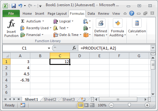
Based on the Excel spreadsheet above, the following PRODUCT examples would return:
=PRODUCT(A1, A2)
Result: 12

=PRODUCT(A1, A2, A3)
Result: 54

=PRODUCT(A1, A2, A3, A4)
Result: -366.12

=PRODUCT(A1, A2, A3, A4, -2)
Result: 732.24
The PRODUCT Excel function is a built-in mathematical function used to calculate the product or multiplication of the given number provided to this function as arguments. For example, if we give the formula arguments 2 and 3 as =PRODUCT(2,3), the result is 6. This function multiplies all the arguments.
The PRODUCT function in Excel takes the arguments (input as numbers) and gives the product (multiplication) as an output. So, for example, if cells A2 and A3 contain numbers, then we can multiply those numbers using PRODUCT in Excel.
Table of contents
- Product In Excel
- PRODUCT Formula in Excel
- Explanation
- Examples
- Example #1
- Example #2 – Nesting of Product Function
- Example – #3
- Recommended Articles
PRODUCT Formula in Excel
=PRODUCT(number1, [number2], [number3], [number4],….)

Explanation
The Excel PRODUCT formula has at least one argument. All other arguments are optional. Whenever we pass a single input number, it returns the value as 1*number, the number itself. The PRODUCT function in Excel is categorized as a Math/Trigonometric function. This PRODUCT formula in Excel can take up to 255 arguments in the later version after Excel 2003. In the Excel version 2003, the argument was limited to only 30 arguments.
The PRODUCT formula in Excel not only takes the input number one by one as an argument but also can take a range and return the product. So, if we have a range of values with numbers and want their product, we can do it by multiplying each one or directly using the PRODUCT formula in Excel, bypassing the value range.

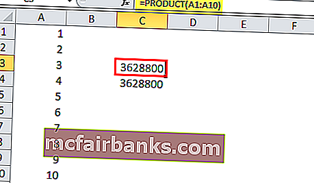
In the above figure, we want to multiply all the values in the range A1:A10. Suppose we use the multiply (*) mathematical operator, it will take much time compared to achieving the same using the PRODUCT function in Excel since we will have to select each value and multiply. Whereas using the PRODUCT function in Excel, we can pass the values directly as a range, and it will give the output.
=PRODUCT(A1:A10)

Therefore, the PRODUCT formula in Excel. =PRODUCT(A1:A10) is equivalent to the formula =A1*A2*A3*A4*A5*A6*A7*A8*A9*A10.
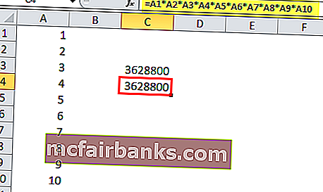
However, the only difference is when we use the PRODUCT function in Excel. If we leave the cell empty, PRODUCT in Excel takes the blank cell with the value 1 but uses the multiply operator. Therefore, Excel will take the value as 0. So, the result would be 0.

When we delete the cell value of A4, Excel considers it as a 0 and returns the output 0, as shown above. But, when we used the PRODUCT function in Excel, it took the input range A1:A10. The PRODUCT function in Excel seems to ignore cell A4, which was empty. However, it does not ignore the empty cell value but takes the blank cell with the value 1. It takes range A1:A10, considers the A4 with value 1, and multiplies the cells’ values. Moreover, it also ignores text values and logical values. The PRODUCT function in Excel considers the dates and numeric values as numbers. Each argument can be supplied as a single value, cell reference, or an array of values or cells.
For small mathematical calculations, we can use the multiplication operator. Still, if we have to deal with a large data set where the multiplication of multiple values is involved, then this PRODUCT function serves a great purpose.
So, the PRODUCT function in Excel is beneficial when we need to multiply many numbers together, given in a range.

Examples
Let us look below are examples of the PRODUCT function in Excel. These Excel PRODUCT function examples will help you explore using the PRODUCT function in Excel.
You can download this PRODUCT Function Excel Template here – PRODUCT Function Excel Template
Example #1
Suppose we have a set of values in columns A and B that contains numeric values with some empty cells. We want to multiply each value of column A with column B in such a manner that if any of the cells have an empty value, we get an empty value. Else, returns the product of two values.

For example, B2 has an empty cell, so the result should be an empty value in cell C2.So, we will use the IF condition along with the OR function. If either of the cell values is nothing returned, nothing else returns the product of the numbers.
So, the PRODUCT formula in Excel that we will use is:
=IF(OR(A2=””,B2=””),””,PRODUCT(A2,B2))
Applying the PRODUCT formula in Excel to each cell, we have:
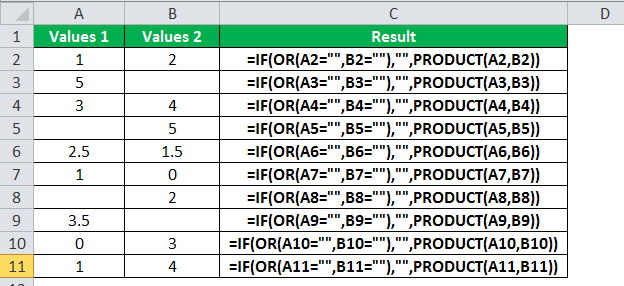
Output:

Example #2 – Nesting of Product Function
When a PRODUCT in Excel is used inside another function as an argument, this is known as the nesting of a PRODUCT function in Excel. We can use other functions and can pass them as an argument. For example, suppose we have four sets of data in columns A, B, C, and D. We want the product of the sum value from the first and second datasets with the sum of values from the third and fourth datasets.

So, we will use the SUM function and pass it as an argument to the PRODUCT function in Excel. We want the product of the sum of the value of “Dataset A” and “Dataset B,” that is, 3+3 multiplied by the sum of the value of “Dataset C.” The“Dataset C,” value is (5+2), so the result will be (3+3)*(5+2).
=PRODUCT(SUM(A2:B2),SUM(C2:D2))

In the above example, the sum function is passed as an argument to the PRODUCT function in Excel. It is known as nesting. But, of course, we can do other functions also.
Example – #3
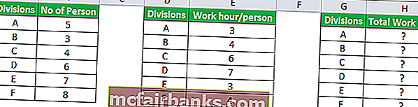
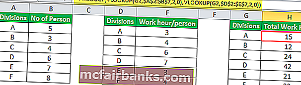
For example, suppose we have six divisions with a different number of persons employed for work. We have two tables with the numbers of persons in each division and the work hour of each person in each division. We want to calculate the total work hour of each division.

So, we will use the VLOOKUP function to lookup the valuesThe VLOOKUP excel function searches for a particular value and returns a corresponding match based on a unique identifier. A unique identifier is uniquely associated with all the records of the database. For instance, employee ID, student roll number, customer contact number, seller email address, etc., are unique identifiers.
read more from both the tables and then pass it as an argument to get the total number by multiplying the number of people by the work hour per person.
So, the formula with Nested VLOOKUP will be,
=PRODUCT(VLOOKUP(G2,$A$2:$B$7,2,0),VLOOKUP(G2,$D$2:$E$7,2,0))

In this way, we can nest the function depending on the requirement and the problem.
Recommended Articles
This article is a guide to the PRODUCT Function in Excel. Here, we discuss the PRODUCT formula in Excel and how to use the PRODUCT Excel function, along with Excel examples and downloadable Excel templates. You may also look at these useful functions in Excel: –
- PRODUCT Formula
- RIGHT Function in Excel | Examples
- IFERROR Function
- POWER Function in Excel
- XOR in Excel
В этом учебном материале вы узнаете, как использовать Excel функцию ПРОИЗВЕД с синтаксисом и примерами.
Описание
Microsoft Excel функция ПРОИЗВЕД Microsoft Excel умножает числа и возвращает произведение.
Функция ПРОИЗВЕД — это встроенная в Excel функция, которая относится к категории математических / тригонометрических функций.
Её можно использовать как функцию рабочего листа (WS) в Excel.
Как функцию рабочего листа, функцию ПРОИЗВЕД можно ввести как часть формулы в ячейку рабочего листа.
Синтаксис
Синтаксис функции ПРОИЗВЕД в Microsoft Excel:
ПРОИЗВЕД(число1;[число2];…)
Аргументы или параметры
- число1;[число2];…
- Числа для умножения. Можно ввести до 30 чисел.
Возвращаемое значение
Функция ПРОИЗВОД возвращает числовое значение.
Применение
- Excel для Office 365, Excel 2019, Excel 2016, Excel 2013, Excel 2011 для Mac, Excel 2010, Excel 2007, Excel 2003, Excel XP, Excel 2000
Тип функции
- Функция рабочего листа (WS)
Пример (как функция рабочего листа)
Рассмотрим несколько примеров функции ПРОИЗВЕД, чтобы понять, как использовать Excel функцию ПРОИЗВЕД в качестве функции рабочего листа в Microsoft Excel:

Hа примере приведенной выше электронной таблицы Excel могут быть возвращены следующие примеры ПРОИЗВЕДОВ:
|
=ПРОИЗВЕД(A1; A2) Результат: 6 =ПРОИЗВЕД(A1; A2; A3) Результат: 22.2 =ПРОИЗВЕД(A1; A2; A3; A4) Результат: —130.98 =ПРОИЗВЕД(A1; A2; A3; A4; —2) Результат: 261.96 |
The Excel PRODUCT function returns the product of numbers provided as arguments. Because it can accept a range of cells as an argument, PRODUCT is useful when multiplying many cells together
The PRODUCT function takes multiple arguments in the form number1, number2, number3, etc. up to 255 total. Arguments can be a hardcoded constant, a cell reference, or a range. All numbers in the arguments provided are multiplied together. Empty cells and text values are ignored.
Examples
The PRODUCT function returns the product of supplied arguments:
=PRODUCT(3,8) // returns 24
=PRODUCT(3,8,4) // returns 96
PRODUCT multiplies all numeric values together, so the following formulas are equivalent:
=PRODUCT(A1:A5)
=PRODUCT(A1,A2,A3,A4,A5)
=PRODUCT(A1:A2,A3:A5)
PRODUCT ignores text values and empty cells. The formulas below will return the same result with all cells have numeric values:
=PRODUCT(A1:A5)
=A1*A2*A3*A4*A5
However, the second formula will return zero (0) if any cells are empty, and a #VALUE! error if any cells contain text.
Notes
- Numbers can be supplied individually or in ranges.
- PRODUCT can accept up to 255 arguments total.
- Only numbers in the array or reference are multiplied.
- Empty cells, logical values, and text in the array or reference are ignored.