
Presentation on theme: «Microsoft Excel.»— Presentation transcript:
1
Microsoft Excel
2
How to Use Tutorial Step 1> The next page will show you the table of contents Step 2> Use the mouse and click on the topic links to begin learning Step 3> You can learn at your own pace, click on the Action buttons to review the material as much as you need to. Step 4> Once you become familiar with this application you can use this tutorial as a reference tool. To begin learning click on this button>>
3
Table of Contents 1_ Introduction to Excel
2_ Overview of the Excel Screen 3_ The Excel Menus: File Menu Edit Menu Insert Menu Format Menu View Menu Help Menu and Office Assistant 4_ Excel Worksheets 5_ Entering Formulas and Data 6_ Formatting Workbooks 7_ Charts 8_ Freezing Panes 9_ Printing 10_ Keyboard Shortcuts
4
Introduction to Excel Excel is a computer program used to create electronic spreadsheets. Within Excel, users can organize data, create charts, and perform calculations. Excel is a convenient program because it allows the user to create large spreadsheets, reference information from other spreadsheets, and it allows for better storage and modification of information. Excel operates like other Microsoft (MS) Office programs and has many of the same functions and shortcuts of other MS programs.
5
Overview of the Excel Screen
Before working with Excel, it is essential to first become familiar with the Excel screen. The following will help you to recognize the various parts of an Excel screen and their functions. The Title bar is located at the very top of the screen. The Title bar displays the name of the workbook you are currently using. The Menu bar is located just below the Title bar. The Menu bar is used to give instructions to the program.
6
Overview of the Excel Screen
Toolbars provide shortcuts to menu commands. There are many different toolbars and the user can choose which toolbars are shown on the screen. To enable more toolbars go to “View” on the Menu bar, select Toolbars, then select which toolbar you wish to add to the screen. The Standard Toolbar provides shortcuts to the File Menu, as well as mathematical functions, chart creation, and sorting. The Formatting Toolbar provides shortcuts to font formatting as well as mathematical functions. The Status Toolbar allows the user to view if the current worksheet is ready to enter data.
7
Overview of the Excel Screen
Microsoft Excel consists of workbooks. Within each workbook, there is an infinite number of worksheets. Each worksheet contains columns and rows. Where a column and a row intersect is called the cell. For example, cell B6 is located where column B and row 6 meet. You enter your data into the cells on the worksheet. The tabs at the bottom of the screen represent different worksheets within a workbook. You can use the scrolling buttons on the left to bring other worksheets into view.
8
Overview of the Excel Screen
The Name Box indicates what cell you are in. This cell is called the “active cell.” This cell is highlighted by a black box. The “=” is used to edit your formula on your selected cell. The Formula Bar indicates the contents of the cell selected. If you have created a formula, then the formula will appear in this space.
9
File Menu When first opening Excel a worksheet will automatically appear. However, if you desire to open a file that you previously worked on go to the “File” option located in the top left corner. Select “Open.” To create a new worksheet go to the “File” option and select “New.” To save the work created go to the “File” option and select “Save.” To close an existing worksheet go to the “File” option and select “Close.” To exit the program entirely go to the “File” option and select “Exit.”
10
Edit Menu Among the many functions, the Edit Menu allows you to make changes to any data that was entered. You can: Undo mistakes made. Excel allows you to undo up to the last 16 moves you made. Cut, copy, or paste information. Find information in an existing workbook Replace existing information.
11
Insert Menu The Insert Menu allows you to:
Add new worksheets, rows, and columns to an existing. You can also insert charts, pictures, and objects onto your worksheet.
12
Format Menu You can change the colors, borders, sizes, alignment, and font of a certain cell by going to the “Cell” option in the Format Menu.
13
Format Menu You can change row and column width and height in the “Row” and “Column” options. You can rename worksheets and change their order in the “Sheet” option. The “AutoFormat” option allows you to apply pre-selected colors, fonts, and sizes to entire worksheets.
14
View Menu The View menu allows you different options of viewing your work. You can enable a Full Screen view that changes the view to include just the worksheet and Menu bar. You can zoom in on your worksheet to focus on a smaller portion.
15
View Menu You can change the view of your work so that it is page by page. You can insert Headers and Footers to your work. You can add comments about a specific cell for future reference.
16
Help Menu and Office Assistant
The Help Menu is used to answer any questions you many have with the program. You can also get online assistance if it is needed. The Office Assistant is a shortcut to the Help Menu. You can ask the assistant a question and it will take you directly to an index of topics that will help you solve your problem.
17
Excel Worksheets With Excel, you will be working with different worksheets within a workbook. Often times it is necessary to name the different worksheets so that it is easier to find them. To do so you must: 1_Double click to highlight an existing worksheet 2_Type in what you would like to rename the worksheet
18
Entering Formulas ADDITION FORMULAS
When entering numerical data, you can command Excel to do any mathematical function. Start each formula with an equal sign (=). To enter the same formulas for a range of cells, use the colon sign “:” ADDITION FORMULAS To add cells together use the “+” sign. To sum up a series of cells, highlight the cells, then click the auto sum button. The answer will appear at the bottom of the highlighted box.
19
Entering Formulas SUBTRACTION FORMULAS
To subtract cells, use the “-” sign. DIVISION FORMULAS To divide cells, use the “/” sign. MULTIPLICATION FORMULAS To multiply cells, use the “*” sign.
20
Tips for Entering Data To highlight a series of cells click and drag the mouse over the desired area. To move a highlighted area, click on the border of the box and drag the box to the desired location. You can sort data (alphabetically, numerically, etc). By highlighting cells then pressing the sort shortcut key.
21
Tips for Entering Data You can cut and paste to move data around.
To update your worksheets, you can use the find and replace action (under the Edit Menu). To change the order of worksheets, click and drag the worksheet tab to the desired order.
22
Formatting Workbooks To add borders to cells, you can select from various border options. To add colors to text or cells, you can select the text color option or the cell fill option, then select the desired color. To change the alignment of the cells, highlight the desired cells and select any of the three alignment options.
23
Formatting Workbooks To check the spelling of your data, highlight the desired cells and click on the spell check button. When entering dollar amounts, you can select the cells you desire to be currency formatted, then click on the “$” button to change the cells. You can bold, italicize, or underline any information in the cells, as well as change the styles and fonts of those cells.
24
Creating Charts With the Excel program you can create charts with the “Chart Wizard.” Step 1: Choose a chart type. Step 2: Highlight the data that you wish to be included in the chart.
25
Creating Charts Step 3: Change chart options. Here you can name the chart and the axes, change the legend, label the data points, and many other options. Step 4: Choose a location for the chart.
26
Freezing Panes If you need the information in one column to freeze, while still being able to scroll through the rest of the data follow these instructions: Step 1: Highlight a specific column. Step 2: Go to the Window Menu and click “Freeze Panes.” Step 3: The cells to the left of the highlighted column should be frozen while you are still able to scroll about the rest of the worksheet (Notice that column A remains while column H is next to it).
27
Printing When printing a worksheet you have a few options.
You can go to “Page Setup” to change the features of your work (the margins, the paper size, the tabs, etc.) This will affect how your project will be printed.
28
Printing You can select “Print Area,” which allows you to only print a highlighted area. You can preview your printing job by selecting “Print Preview.” Finally, you can print your job by going to the File Menu and selecting “Print,” or you can use the shortcut button.
29
Keyboard Shortcuts Here are some basic keyboard shortcuts:
Shift + arrow key = highlight information CTLR + A = Select All CTRL + C = Copy Information CTRL + X = Cut Information CTRL + V = Paste Information CTRL + Z = Undo Information HOME = Move to the beginning of the worksheet
30
Notes to the teacher: This curriculum was designed so that it could be easily modified by the teacher. The teacher can add slides at any point in the curriculum depending on the level of computer literacy of the students. The Basic Outline of the curriculum is to be used as a guidance tool and will help the teacher create a syllabus for the class being taught. Slides that are blank are topics we deemed important but not necessary to have included in the curriculum. These slides were considered advanced topics. (please ignore if there are no blank slides) You can choose to add content to these slides or to delete them.
Слайд 1
Описание слайда:
Презентацию подготовила:
Презентацию подготовила:
Студентка 103 группы лечебного факультета
Марочкина А.Н.
Преподаватель:
Колпакова М.А.
Слайд 2
Описание слайда:
Содержание
Что такое Microsoft Excel
История создания
Создание, загрузка и сохранение фалов — документов.
Окно программы MS Excel
Функции MS Excel
Стандартные функции MS Excel
Заключение
Слайд 3.
Microsoft Excel входит в состав Microsoft Office и на сегодняшний день Excel является одним из наиболее популярных приложений в мире.")
Описание слайда:
Что такое Microsoft Excel
Microsoft Excel-программа для работы с электронными таблицами, созданная корпорацией Microsoft.
Она предоставляет возможности экономико-статистических расчетов, графические инструменты и, язык макропрограммирования VBA (Visual Basic for Application).
Microsoft Excel входит в состав Microsoft Office и на сегодняшний день Excel является одним из наиболее популярных приложений в мире.
Слайд 4
Описание слайда:
История создания
Какова же история создания столь мощного инструмента для вычислений? Всё началось с того, что в 1982 году компания Microsoft выпустила 1-ый табличный процессор под названием Multiplan, который завоевал огромную популярность среди CP/M систем. Самая 1-ая версия Excel появилась на компьютерах Mac в 1985 году.
А 1-ая версия для Windows стала доступна лишь в ноябре 1987 года. Компания Microsoft решила не останавливаться на достигнутом и год за годом укрепляла свои позиции на рынке и выпускала новые, всё более совершенные версии электронных таблиц Excel.
Слайд 5
Описание слайда:
Создание, загрузка и сохранение фалов — документов.
После запуска MS Excel по умолчанию предлагает вам начать создание нового документа под условным наименованием Книга 1.
Можно подготовить документ, а затем сохранить его на диске в виде файла с произвольным именем и расширением.XLS. Сохранение файлов – документов выполняется по стандартным правилам Windows.
Слайд 6
Описание слайда:
Окно программы MS Excel
Окно содержит все стандартные элементы: заголовок, горизонтальное меню, две панели инструментов, полосы прокрутки, строка состояния.
Как и в Word, выдаваемые вами команды применяются либо к выделенной ячейке, либо к выделенному блоку ячеек, либо ко всей таблице.
Ниже панели «Форматирование» располагается строка формул, в которой вы будете набирать и редактировать данные и формулы, вводимые в текущую ячейку.
В левой части этой строки находится раскрывающийся список именованных ячеек, и заголовок этого списка называется полем имен. В этом поле высвечивается адрес выделенной ячейки таблицы.
Слайд 7
Описание слайда:
Функции MS Excel
Функции задаются с помощью математических и других формул, которые выполняют вычисления над заданными величинами, называемыми аргументами функции в указанном порядке, определяемом синтаксисом.
Список аргументов может состоять из чисел, текста, логических величин, массивов, значений ошибок или ссылок. Необходимо следить за соответствием типов аргумента. Кроме того, аргументы могут быть как константами, так и формулами. Эти формулы, в свою очередь, могут содержать другие функции. Ввод формул можно выполнить либо непосредственно в ячейке, либо в строке формул.
Слайд 8
Описание слайда:
Стандартные функции MS Excel
Стандартные функции в MS Excel подразделяются на следующие основные группы:
Финансовые;
Функции для работы с датами и временем;
Математические;
Статистические;
Функции для работы со ссылками и массивами;
Функции для работы с базами данных;
Текстовые;
Логические;
Функции для проверки свойств и значений.
Слайд 9
Описание слайда:
Заключение
Программа Microsoft Excel представляет собой электронную таблицу, которая состоит из строк и столбцов.
Запускается эта программа, любым из стандартных способов. В Microsoft Excel файлы можно создавать, загружать и сохранять.
Excel позволяет разделить окно таблицы на два или четыре подокна и одновременно работать с разными частями одной и той же таблицы.
Окно программы по структуре похоже на окно программы MS Word. Оно содержит все стандартные элементы: заголовок, горизонтальное меню, две панели инструментов, полосы прокрутки, строка состояния.
Также в этой программе можно произвести настройку экрана.
Слайд 10
Описание слайда:
СПАСИБО ЗА ВНИМАНИЕ!
Содержание
- Презентация на тему: Microsoft Excel
- Microsoft Excel.
- Similar presentations
- Presentation on theme: «Microsoft Excel.»— Presentation transcript:
- Introduction to Microsoft Excel
- Similar presentations
- Presentation on theme: «Introduction to Microsoft Excel»— Presentation transcript:
Презентация на тему: Microsoft Excel
Microsoft Excel Использование встроенных функций. Формулы, их копирование, расчеты
Все о формулах Формула выполняет вычисления соответствующих заданий и отображает на листе окончательный результат; В формулах Excel можно использовать числа, знаки арифметических действий и ссылки на ячейки; Формула ВСЕГДА начинается со знака равенства(=); По умолчанию формулы на экране не отображаются, но можно изменить режим работы программ, чтобы увидеть их; Формулы могут включать обращение к одной или нескольким функциям; В формулах недопустимы пробелы; Длина формулы не должна превышать 1024 элементов; Нельзя вводить числа в форматах даты и времени дня непосредственно в формулы. В формулах они могут быть введены только в виде текста, заключенного в двойные кавычки. Excel преобразует их в соответствующие числа при вычислении формулы.
Ввод формулы Щелкните ячейку, в которую нужно ввести формулу; Введите знак равенства — обязательное начало формулы. Введите первый аргумент — число или ссылку на ячейку. Адрес можно ввести вручную или вставить автоматически, щелкнув нужную ячейку; Введите знак арифметического действия; Введите следующий аргумент; Повторяя пункты 4 и 5, закончите ввод формулы; Нажмите Enter. Обратите внимание, что в ячейке отображается результат вычислений, а в строке формул — сама формула.
Вывод формул на экран Выберите из меню Сервис команду Параметры; Щелкните вкладку Вид; Установите флажок Формулы; Щелкните OK. Вычисление части формулы При поиске ошибок в составленной формуле бывает удобно посмотреть результат вычисления какой-то части формулы. Для этого: Встать на ячейку, содержащую формулу; В строке формул выделить часть формулы, которую нужно вычислить; F9 — вычисление Enter – результат вычисления выводит на экран Esc — возврат формулы в исходное состояние.
Совет При вводе формул необходимо учитывать приоритет арифметических операций. В Excel порядок старшинства операций таков: возведение в степень; умножение и деление; сложение и вычитание. Например: D1 равно 28
Виды ссылок на ячейки В формулах Excel обычно использует относительные ссылки. Отсюда следует — ссылки в формулах автоматически изменяются при копировании формул в другое место. Например, если в ячейке B10 содержится формула = СУММ (В3:В9), то при копировании этой формулы в ячейку С10 она преобразуется в =СУММ (С3:С9). Чтобы ссылки в формуле не изменялись при копировании формулы в другую ячейку, необходимо использовать абсолютные ссылки. Абсолютная ссылка обозначается знаком доллара ($), который располагается перед номером строки или обозначением столбца. Например, комиссионный процент по продажам помещен в ячейку D7, тогда абсолютная ссылка на ячейку должна выглядеть как $D$7. Абсолютная строка выглядит как D$7. Абсолютный столбец выглядит как $D7.
Перемещение и копирование формул Формула введена в ячейку. Её можно перенести или скопировать. При перемещении формулы в новое место таблицы ссылки в формуле не изменяются. При копировании формула перемещается в новое место таблицы: а) ссылки перенастраиваются при использовании относительных ячеек; б) ссылки сохраняются при использовании абсолютных ячеек.
Формулы: Замена значениями Формулу на рабочем листе можно заменить её значением, если в дальнейшем понадобится только результат а, а не сама формула. Для этого: Выделите ячейку с формулой, которую нужно преобразо- вать в значение; Щелкните на кнопке Копировать на стандартной панели инструментов; Выберите Правка — Специальная вставка и щелкните на строке Значения. Щелкните на ОК; Нажмите Enter, чтобы убрать «муравьиную дорожку» вокруг ячейки.
Формулы: защита и скрытие Защита ячеек предотвращает изменение или уничтожение важной информации. Также возможно указать, следует ли отображать содержимое ячейки в строке формул. Чтобы снять защиту ячейки (диапазона ячеек) или запретить отображение её содержимого в строке формул, сначала выделите нужную ячейку или диапазон; Выберите Формат — Ячейки и щелкните на вкладке Защита; Снимите флажок Защищаемая ячейка, чтобы снять защиту ячейки. Установите флажок Скрыть формулы, чтобы они не отображались в строке формул при выборе ячейки. Щелкните на ОК; Установите флажок Сервис – Защита – Защитить лист. Результат – весь лист, кроме изменяемых ячеек, защищен
Формулы: создание текстовой строки Иногда бывает нужно объединить содержимое двух ячеек. В Excel такая операция называется конкатенация. Для этого: Выделите ячейку, в которую нужно поместить формулу и введите знак равенства (=), чтобы начать ввод; Введите адрес или имя или щелкните на ячейке на рабочем листе; Введите оператор конкатенации (&), затем введите следующую ссылку; Если необходимо, повторите шаг 3. Не забывайте о том, что в формулу необходимо вставить кавычки с пробелом между ними, чтобы Excel вставила пробел между двумя текстовыми фрагментами. Чтобы закончить ввод формулы, нажмите Enter. Пример: формула=С3&” “D3, где С3- «Парафеева», а D3 — «Таня» Даст результат : «Парафеева Таня» — в одной ячейке
Формулы: ссылки на ячейки из других рабочих листов. При организации формул возможно ссылаться на ячейки других рабочих листов. Для этого: Выделите ячейку, в которую нужно поместить формулу, и введите знак равенства (=); Щелкните на ярлычке листа, содержащего нужную ячейку; Выделите ячейку или диапазон, на который нужно установить ссылку. В строке формул появится полный адрес; Завершите ввод формулы, затем нажмите Enter. Пример: формула = Лист1!В6+Лист2!D9
Все о функциях Функциями называют встроенные в Excel формулы; Функций в Excel сотни: инженерные, информационные, логические, арифметические и тригонометрические, статистические, функции обработки текста, функции работы с датой и временем, функции работы с базами данных и многие-многие другие; Функции можно использовать как по отдельности, так и в сочетании с другими функциями и формулами; После имени каждой функции в ( ) задаются аргументы. Если функция не использует аргументы, то за её именем следуют пустые ( ) без пробела между ними; Аргументы перечисляются через запятую; Функция может иметь не более 30 аргументов.
Ввод функции Щелкните ячейку, в которую хотите ввести функцию; Введите знак равенства, название функции (или выберите из Мастера функций) и открывающуюся круглую скобку; Введите аргумент или щелкните ячейку или диапазон, которые нужно использовать при вычислении функции; Щелкните кнопку ввода в строке формул или нажмите Enter. Закрывающуюся скобку Excel вставит самостоятельно.
Самые популярные функции Excel
Функции: мастер функций Мастер функций выводит на экран список функций, из которого пользователь может выбрать нужную функцию. Для этого: Выделите ячейку, в которую нужно поместить функцию, и щелкните на кнопке на стандартной панели инструментов; Укажите нужный тип функции в списке Категории. Если вы не знаете, к какой категории принадлежит функция, выберите 10 недавно использовавшихся или Полный алфавитный перечень; Выберите конкретную функцию из списка Функция. Прочитайте описание в нижней части окна диалога, чтобы убедиться, что функция выбрана правильно, затем щелкните на ОК. Под строкой формул появится окно, так называемая палитра формул. Введите аргументы в соответствующие поля. Вы можете вводить значения или адреса ячеек вручную, можете щелкать на нужных ячейках или выделять нужные диапазоны; Щелкните на ОК, чтобы завершить ввод функции и поместите её в ячейку.
Источник
Microsoft Excel.
Published byMarcia Booker Modified over 4 years ago
Similar presentations
Presentation on theme: «Microsoft Excel.»— Presentation transcript:
2 MS Excel Microsoft Excel: is a special office program used to apply mathematical operations according to reading a cell automatically, just click on it. It is called electronic tables
3 Starting Excel application
To start MS . Excel do the following: From the Start button on the taskbar , select All Programs. Select Microsoft Office then select Microsoft Office Excel
4 Microsoft Excel windows Elements
Office Button Cell Name Formula Bar Wrap Text Title Bar Auto Sum Auto Fill Merge and Center Cell Column headings Row headings Sheets Worksheet
5 MS Excel To create a new Workbook, do the following:
Click on the Office button click New. To save the workbook, Click the office button then Save as
6 MS Excel To rename worksheet, do the following:
Right click on the worksheet which you want to rename. Click on (Rename) to allow you to write the new name. Write the demanded name then press (Enter) to apply the name.
7 MS Excel To insert the worksheet, click on this button
To order the worksheet, click on the sheet which you want to change its location, then start to drag while pressing on left button of mouse. To delete the worksheet, , do the following: Right click on the worksheet which you want to delete. Click on (Delete).
8 MS Excel To insert rows or columns in worksheet, do the following:
To delete rows or columns from any where in worksheet, do the following: Click on the Home tab, In the Cells group , Click delete. To insert rows or columns in worksheet, do the following: Click on the Home tab, In the Cells group , Click Insert.
9 MS Excel To justify the height of rows, do the following:
Click on the Home tab, In the Cells group , Click Format. Then from the Cell Size menu select (Row Height) In the dialog box: write the demanded height then click OK To justify the width of columns, do the following: Then from the Cell Size menu select (Column Width) In the dialog box: write the demanded width then click OK
10 MS Excel To change the direction of the whole worksheet from right to left or to the opposite: Click on the Page layout tab, In the Sheet options group , Click
11 MS Excel To enter a text or a number on any cell:
click on the cell using the mouse start to use keyboard buttons to write then press Enter. To enter a date or time on any cell: Click on the Home tab, In the Number group Select data, then choose date or time from list.
12 MS Excel To edit the content of any cell, do the following:
Double click on the cell which you want to edit. Then write the demanded text in the cell. To copy or cut the text, determine the text then press To delete the content of cell , click on the demanded cell and then press (Delete)
13 MS Excel to fill the text to other cells on the worksheet, do the following: Click on the cell which you want to fill its content (text/number) to others. Adjust the mouse cursor on the box appearing on the lower right corner, then begin to drag with continued pressure on the left button in the direction that you want to fill the text through.
14 MS Excel Freeze panes: To apply the freeze order, follow these steps:
Click on the cell from which you want to start freezing Click on View tab, then select (Freeze panes)
15 MS Excel To hide worksheets, columns and rows
Click on the Home tab, In the Cells group , Click Format. Then from Visibility menu, select Hide & UnHide.
16 MS Excel Formatting text: Aligning text in cell
Font Size , Font Color, Font type , Bold ,Italic Background color Sort & Filter Aligning text in cell
17 MS Excel Using the style buttons to format Numbers.
Applying conditional formatting Adding Border and shading
18 Performing Simple Calculations
+ , — ,* , /
19 Performing Calculation with Functions
Sum Max (Maximum Value) Min (Minimum value) Average IF count
20 Charts To insert chart , do the following:
Select the column or row which you want to insert a chart for. Then click on insert tab, In the charts group click a chart that you want to use.
21 Chart If you want to change the of the chart after inserting it, click Design tab then select Change Chart Type Control the size of a chart. Chart Title, axis Title. Layout Tab-> Chart title Layout Tab-> axis title
22 Printing your Workbook
Источник
Introduction to Microsoft Excel
Published byKelly Hodge Modified over 7 years ago
Similar presentations
Presentation on theme: «Introduction to Microsoft Excel»— Presentation transcript:
1 Introduction to Microsoft Excel
Objectives: To define spreadsheets and explain basic functionality To introduce the basic features of Excel Vocabulary Entering Data Formatting Data Precision vs. Display Operators & Order of Precedence For those of you who have never used Excel or any other spreadsheet software application – many of these techniques and concepts will be new. We have provided both videos and reading to get you up to speed on the basics of these types of software packages and in specific Excel. For those of you whom have used spreadsheet software.. Some of this may be a review.. but perhaps not all. Like last class – it helps to know something about the tools you’re using to understand the types of results.
2 Spreadsheet: Electronic sheet of paper organized by columns & rows
The advantage of an electronic spreadsheet is it allows you to easily change data and have all “related” calculations automatically update.. Excel is basically a software package that allows you to easily work with data in a grid-like format using columns and rows to display information. Being ‘electronic’ there are many features that make it easier to use than the pencil and paper version – the most notable is the ability for our spreadsheets to be automatically recalculated if any of the data inputs are later updated – but for this to happen we will need to learn how to properly setup and write spreadsheet formulas
3 Active Cell displayed on Formula Bar
Spreadsheets in Excel are referred to as worksheets. A workbook file may contain may worksheets. Sizing Buttons Help Button Quick Access Toolbar Home Ribbon Ribbon Tabs Formula Bar Name Box Column Letter Headings Fx Insert Function Button Contents of Active Cell displayed on Formula Bar Row Numbers Scroll Bars This is a brief overview of the Excel window with the home ribbon displayed. For those not familiar with this version of Excel – I recommend you use the SAM tutorials to catch up – you will be responsible for knowing the terminology presented and being able to correctly identify/use the various worksheet features. The center of the Excel window is the worksheet and worksheet cells – with the row numbers displayed on the left and column letters above. Just above the column letters are two boxes – the name box which we will use later to give a name to a cell or range of cells – and the formula bar. When you click on a specific cell — the contents of this active cell will be displayed in the formula bar. If the value 5 is typed into the cell this value will appear in the formula bar – however if the value 5 is a result of a calculation – the cells typically displays this value but the formula bar will list the actual formula that was written and is saved to this cell. Notice that just to the left of the formula bar is the FX button – which launches the function wizard – as we will see later. Just above the name box and formula bar is the ribbon. Which ribbon is displayed will be determined by which ribbon tab is selected.. The tabs are just above the ribbon buttons – seen here is the home ribbon. Each ribbon is further subdivided into common tool groups such as Clipboard, Font, Alignment etc. Above the ribbon on the left is the quick access toolbar – which you can customize as you see fit – this toolbar is always visible – so regardless of which ribbon is displayed the buttons placed on the quick access toolbar are always one click to use. In a similar manner the sizing buttons for the Excel application window and for the spreadsheet window and the help button are displayed on the upper right hand side. To maneuver within the spreadsheet you can using the up/down arrow keys – move your mouse or click on the horizontal or vertical scroll bars at the bottom and sides of the worksheet. You can also go from one worksheet to another using the sheet tabs at the bottom. On the bottom right of the worksheet window is the zoom tool to help you easily change the size displayed on your screen w/o impacting the font size used within the spreadsheet – which determines print sizes. Sheet Tabs Insert Worksheet Button View Buttons Zoom
4 Each box is referred to as a “cell”
Each box is referred to as a “cell”. Cells may contain Labels, Values or Formulas that result in a value or label. A cell is identified first by its column letter and then by its row number Columns Cell D2 Contains the Formula = B2*C2 Rows Labels Again each box is referred to as a cell and the selected cell is referred to as the ‘active cell’ – When a cell is active — its contents will be displayed in the formula bar. Columns are labeled with letters A,B,C.. At Z they begin again with AA…eventually going to XFD or more. Rows are sequentially numbered from 1 to past 1 million. The number of rows and columns available on the spreadsheet are limited to your computer’s available RAM memory. Cells are identified first by their column letter and then by their row number. The cell containing the title ‘food item is referred to as cell A1. Cells may contain either labels, values or formulas which result in labels or values. Labels are text such as seen in cell A4 – which contains the word ‘eggs’. Cell B2 contains a value — a number which was directly entered into the cell in this case 2.5. Cell D2 contains a formula =B2*C2 resulting in the value 5 – the product of the values contained in cells B2 and cells C2 – the resulting value will normally be displayed in the cell, however when this cell is selected the underlying formula will be display in the formula bar.
5 One can also write formulas that refer to cells on other worksheets – Sheetname!Cell-Reference
input!B1*input!B3 + A1 When referencing a cell on the same spreadsheet as the active cell the sheet name is not required. A workbook can contain any number of worksheets which can be accessed via the corresponding sheet tab. When working on a single worksheet we address a cell reference by its column letter then row.. Such a A1 or E5. When working on multiple worksheets we must refer to cells on different worksheets by prefacing their column and row address with a worksheet name. If you were to write a formula on sheet1 – sheet1 is referred to as the active worksheet. Cells referenced on sheet 1 would not require a sheet name, cells referenced on other worksheets would require their sheet name in addition to their row and column address. For example the formula input!B1*input!B3 +A1 would multiply the value on sheet input in cell B1 with the value on sheet input in cell B3 and then add the value A1 from the active worksheet where the formula is currently being entered. Also note the syntax of cell referencing using sheet names required an exclamation point following the sheet name. In a few moments we will demonstrate how to insert worksheets, modify the sheet tab names and colors and how to input formulas on our worksheets. Sheets may be named and displayed with different colors tabs, The order of the worksheets may be modified as well.
6 File tab – opens menus for opening and
saving Files, and modifying Excel Options Quick Access Toolbar can be customized to include icons to frequently Used features such as Print Preview Home Ribbon use to change fonts, justify text, insert rows etc. Ribbons are organized into Groups of similar tasks such as the Font group or the Number group. In addition, there are other ribbons containing groups/buttons for laying out pages using the review features etc. Here’s a closer look at the home ribbon , tab and quick access toolbar elements. What I suggest – for those who don’t use excel on a daily basis – go in and click on each ribbon tab – look over some of the tool buttons – try them out. The File tab unlike the other ribbon tabs – launches what is referred to as the backstage view – essentially a menu for saving, opening, closing files and for accessing spreadsheet properties –options that can be modified such as how certain keys work, what language is used, and even spreadsheet security.
7 Highlight your data, select a Chart type and Edit & its done!
Another feature of Excel that is basic to its use is creating graphs – to create a simple chart as seen above – just highlight the data – select the chart from the insert ribbon and its done. Of course we’ll spend some additional time talking about charts later this semester – but if you don’t know how to do a simple one – again use SAM tutorials provided for help.
8 The “Power” of using Spreadsheet Applications
=B2*C2 Each entry can be related to other values by including cell referencing in formulas. Formula values are automatically updated when a referenced value changes Formulas can be copied Charts can be easily generated One of the great advantages of using an electronic spreadsheet is that we can setup formulas that reference cells containing our data. As we saw in the demo, By doing this – if the data is later modified these calculations will be automatically updated. In this example, if the price of carrots in cell B2 was increased from $1 to $2 both cell D2 the total cost of carrots and cell D4 the total cost of all items would be automatically updated. Another advantage of using an electronic spreadsheet such as Excel, is that it also enables the user to quickly and easily create charts from this data such as the one seen here on this slide. And later on in Excel we will see how we can copy elements of a worksheet – to make them simpler to create But in order to take advantage of these spreadsheet features we must write formulas correctly. Our formulas serve as basic instructions telling Excel what we want to do.
9 Formulas always start with an equal sign =
A formula is a sequence of values, cell references and operators that produce a new value. = E8 + 3*(E10 — E11) Formulas always start with an equal sign = In addition a formula can also contain built-in functions like SUM, AVERAGE, IF, COUNTIF, etc. =Sum(A2:A8)*2 First lets formally define what a formula is in EXCEL: A Formula is any sequence of values, cell references and operators ..such as addition, subtraction, or multiplication that produce a new value.. Seen here is a formula that will add the contents of cell E8 to 3. Notice that a formula begins with an equal sign. To alert Excel that you wish to enter a formula and not a label or value – you must preface a formula with an equal sign. Formulas may also contain functions – which are sort of built in shortcut calculations such as SUM or Average. Using and writing functions will be the topic of future lectures
10 Things you need to know when writing formulas in Excel
Data precision vs. cell display Types of operators that can be used Order of precedence of operators / ≤ − What else do we need to know in order to write an Excel formula? Consider for example if we want to tell Excel to multiply two values and one of the values is the result of a previous subtraction such as multiply 3 by the difference of the values in cells E10 and E11 – (write out words on callout) How do we tell Excel to multiply two values, and how do we indicate that we want the subtraction performed BEFORE the multiplication. To understand how write this formula so that we get the desired result we will now learn about the types of operators available in Excel and their representative symbols, and how the order of these operators will affect our resulting values. We will also discuss the difference between Data Precision and Cell Display to see how these will impact what we view on the worksheet. =B2+B3*B1/B8^2
, =, ,=» > 11 Relational operators: >, =, ,=
In order to write Excel formulas we also need to use the correct Operator Symbols Formulas contain two types of components: Operators: Operations to be performed Arithmetic operators: * / + — ^ Relational operators: >, =, ,= Operands: Values to be operated on Addition Operator Formulas are composed of two elements – operators and operands…the values we require and the operations we wish to perform on them. The Arithmetic operators available to us in Excel include addition – represented by a plus sign, subtraction represented by a minus sign, multiplication represented by an asterisk, division represented by a slash and exponentiation represented by the hat symbol found above the value 6 on most keyboards. (use a callout for this list) In the example here, the operands B2 and 5 are acted on by the addition operator. To perform this operation, Excel will take the value in cell B2 and add it the value 5. In addition to arithmetic operators Excel provides relational operators the greater than relationship is represented by the greater than symbol usually found above the period on the keyboard The less than relationship is represented by the less than symbol The greater than or equal to relationship is represented by typing the symbol greater than immediately followed by and equal sign And the less than or equal to relationship is represented by typing the symbol less than immediately followed by and equal sign A less than sign followed by a greater than sign represents a ‘not equal to’ relationship To represent an equal to relationship the equal sign is used as seen here (callout =B2=5) – here the first equal sign indicates a formula will follow and the 2nd indicated that the values B2 and 5 be tested to see if they are equal. We will be using these relational operators later in this course when we discuss Boolean logic. = B2 + 5 Operands
12 Precedence of Operators
( ) Parenthesis is a special operator that forces evaluation of the expression inside it first Exponentiation (2^3 8) Arithmetic operators: Multiplication & Division Multiplication & Division have equal precedence and are evaluated from left to right Arithmetic operators: Addition & Subtraction Addition & Subtraction have equal precedence and are evaluated from left to right Relational operators have a lower precedence than arithmetic operators Which operation is performed first is prescribed by the order of the precedence rules.. Similar to those you learned in algebra.. Remember the computer is very consistent about applying those rules.. So on a math test if you forgot to write a parenthesis, but you knew what you were doing…you might still end of with the correct answer.. But not here…Excel will only do exactly what you tell it to do! The prescribed order of operations are as follows: First are foremost – operations in parentheses will be performed. Next in order is Exponentiation – Division and Multiplication follow with equal precedence ..evaluated from left to right..so in the formula =25/5*2 will first divide twenty five by five and then multiply by 2 resulting the value 10 – if you had wanted to perform the multiplication of 5*2 first and then divide 25 by the resulting value 10 to get 2.5 – you would need to include parentheses (use a callout) Next in order of precedence are the arithmetic operators of addition and subtraction – again they have equal precedence and are evaluated from left to right. And last to be evaluated will be relational operators such as greater than, or less than.
13 Precision: number of decimal places stored in the computer.
Formatted Display: number of decimal places that appear in a cell Does the addition appear to be correct in col B? Type in a cell : =1/8 display in cell What value results for each — if multiplied by 1000? Displayed on this slide are two sample spreadsheets. Consider the one on the left where the formula = 1 divided by 8 has been placed in cells B1 through B4. Cell B1 has been formatted using the Increase/Decrease decimal toolbar to show zero decimal places and thus 1/8 is displayed as a zero. In cell B2 we show this same value displayed with 1 decimal place, in row 3 with 2 decimal places and finally in row 4 with three decimal places. What value would result if we write another formula = B1 *100..(put in callout)? At first glance it might seem like the computer would perform the computation zero times And get a result of zero. But such is not the case. Even though the displayed value in cell B1 is zero.. The actual value stored by the computer is still the calculation of one divided by eight or Thus the result of this formula would be 12.5. The difference between the displayed value and the precise value stored in a cell can sometimes cause confusion .. Consider the example in the right box of this slide. Here the identical values were entered in cells a2 to a4 as in cells b2 to b4.. But they are displayed with a different number of decimal places. Upon first glance if you were to add the values in column B.. It seems that the resulting value is just plain wrong.. Adding the ones column we have this should give use a zero in the ones column ..eventually resulting in the value 170 not Clearly your boss might think either you don’t know what you’re doing or Excel has some sort of ‘bug’ and just can’t add. In truth we need to be careful to display appropriate numbers of decimal places when presenting data – and most importantly to be aware that the differences are often attributable to rounding of the displays and not the actual values stored – and thus not cause for panic.
14 Formatting affects display not the precise value:
Formatting Number Group Percent Decimal Display Currency Commas Indeed there are several ways to change a number’s format without actually changing the precise value stored in a cell. In cell E2 for example is the calculation 4 divided 6.34 (show callout =d2/d4) results in the value When its displayed in percentage format.. The cell will contain the numerals 63 with a percentage sign… however the precise value stored is still if you multiply cell E2 by 100 you will get 63 not (have call out .63*100 vs. 63*100) The currency format will display a dollar sign symbol and 2 decimal places.. again w/o changing the precise value stored. Excel even gives us an option to display commas..
15 Values can also be used to display dates
Dates are values that can be entered in several formats: January 27, 2013 or 1/27/2013 Excel converts these dates to a numerical representation (1/22/2013 41301) Thus dates may be used in formulas: =A1–B1 will result in the value 5 Excel also has a facility for storing dates. If you type into a cell ‘1/27/2013’ for example without an equal sign – normally Excel will perceive that this entry is a date and store it as such. In a similar manner if you enter the text february 1, 2013– Excel will also most likely perceive this to be a date. Dates entered in a ‘date format’ are converted into values…based on a precise mathematical formula – where January 1, 1900 is the value 1 and each succeeding day is one more than the previous. This allows us to perform arithmetic operations on dates.. So for example you calculate the date it will be five days from today or the number of days it took to ship an item if you have both the ship date and received date. While these dates are stored as numbers – they can be displayed in a variety of formats which can be specified from the Format Cells Number tab. Now in cell C1 lets subtract the 2 dates to see how many days lie between them..=b1-a1. You might end up with the value 5 or some strange answer like January 5, What is going on? Actually – the precise values of these two displays are actually the same. But somehow Excel decided to display the value as a date – when we actually wanted a number display. In some cases the opposite can happen – if you add 5 days to a specific date – at times you might erroneously get a number instead of a new date. To correct this problem we can modify the cell display. To change the cell display use the Format menu and select Cells and the Number tab of the dialog box. Then choose the correct display in this case the Number format Also note that dates cannot be typed directly in a formula. If you write 1/27/2013-1/22/2013 directly into a cell ..the computer will interpret this as 1 divided by 27 divided by To subtract these dates you will need to enter each individual date into a cell – say place jan 27 in cell a1 and jan 22 in cell b1 and then write the formula a1-b1! Note: To do arithmetic calculations with dates if you type =1/27/2013-1/22/2013 directly in a cell it does not interpret it a date – cell references must be used.
16 Walkthrough: Building a Simple Spreadsheet
Entering labels and values Formatting cells font, size, style, color, borders, alignment Numeric Format, Currency, Decimal Places text wrap, center titles Column widths, row height Inserting/Deleting rows and columns and sheets Writing a simple formula & modify decimal display Create a simple chart Sheet tabs Creating a new worksheets in a workbook (“new sections in a document”, Naming Sheets Create the worksheet similar to the Foods worksheet for this week problems.. Demonstrating each of the feature listed here: Lets switch now to a new worksheet and begin learning how to enter data, format our cells, insert and delete columns, rows and worksheets as well demonstrate how to write simple formulas. Use spreadsheet: Consider the Simple formulas spreadsheet available in your course notes – similar to the one we’ve used in our slides listing food quantities and prices(show original spreadsheet for a moment). Lets try to re-create some of these elements beginning with a new worksheet. (follow steps) To launch EXCEL click on the start menu and select Excel.. If its not pinned to your menu then select ‘all programs’ ‘microsoft office’ and then excel. Here is our workbook: Note the ribbons, scroll bars and worksheet tabs. In cell A1 lets type ‘food item’ — To type in a cell first select it by clicking you mouse in the desired location. When you’re done typing click enter to — the active cell is then changed to the cell below what you’ve just typed. Now lets type cereal then enter, milk, cheese, and meat. (type in make error typing ‘mead’ Unfortunately I’ve incorrectly typed the word ‘meat’ – to correct an error while your still typing you can use the backspace key as seen here.. Or you can use your mouse to highlight parts of the text to delete or type over, or use click between 2 letters to insert text. One can also create line breaks within a cell wrapping the text to automatically size to the column.. Use the Wrap Text button on the Home ribbon. You wrap the text at a specific point double clickon the cell, which gets you into the edit mode, and then place the cursor where you’d like a new like and typing Alt Enter. Now lets fill in column B — to move to different cells you can use either the mouse or the up/down arrows on your keyboard. In cell B1 lets type price per package, and the values 2.5, 1.5, 3.5, 3.75. Our new spreadsheet contains may of the elements of the original – but looks completely different. Shown here are the two worksheets side by side – consider the differences- For one thing the text of the original is larger, darker and in some places italicized. Row 1 is in yellow and the other rows are highlighted in grey. The title in column B seems to extend over the line and doesn’t wrap around as in our original worksheet. All of these elements can be modified using the formatting tools. First lets change the font size of cell A1 to 12 and bold the text using the Bold button on the Font group of the home ribbon. This ribbon group can be used to italicize, underline, capitalize text. Or to change font or font sizes. The Paragraph group buttons can be used to align the text. Even more options are available by launching the format dialog box from the launch button located at the bottom-right of the ribbon group Use the fill color button on this same ribbon group to change the cell color to yellow. Now that we’ve done all of this formatting in cell A1 – will we need to do it again and again for each cell on my worksheet? If you select multiple cells at once you can simultaneously set the formats for all selected cell. But since we didn’t originally do that, we can accomplish this by copying only the cell format in cell A1- without actually copying the contents. A neat tool that will allow you to do this is the format painter.. Click on the cell you wish to emulate, then click on the ‘paintbrush’ toolbar button. One click will let you copy this format to a single selection – double clicking will allow you to copy the format to multiple selections. Here we’ll click once.. Notice the cursor turns into a paintbrush.. Now click on cell B1.. And the format is copied. Note that these formats are not linked – if you later change the format in the original cell.. It will have no affect on any other cells. (demo by changing format).. By the way to undo an action use the ‘undo’ toolbar button – this is also available from the edit menu. Now consider the values we typed in column B, notice that on the original worksheet all values contain 2 decimal places and are lined up by their decimal point. To accomplish this we can again use the tool buttons on the Number group of the Home ribbon. first selecting the range of cells we wish to format – (demo select cells, format, cells, number) then select the , button to select comma style. This automatically provides 2 2 decimal places – and for larger number thousands separators. To increase or decrease the number of decimal places you can also use the increase/decrease decimal buttons or go into the formatting dialog box and select another options. Another difference between the 2 worksheets is the width of column B and how the title price per package is laid out. Just place your cursor on the column heading line between B and C and drag. To exactly size a column to fit the widest text in that column double click on the line Notice that when we did this – the title still appears on one line. To wrap the text of the title to fit on multiple lines within a cell – we can again use text wrap button. Not complete Now lets add the number of packages in column C – first by typing our label in cell c1, #pkgs, and then by – typing in 2,1,2,1 in cells C2:C5 use the increase/decrease buttons to format the values To complete the formatting of the new worksheets lets italicize and bold column A (bold, italicize column A), Lets bold bold columns B and C (highlight b2:c5 – click on bold toolbar button). Lets copy the format from column B title to column C title by using the paintbrush and then lets change the background of cells a2:c5 by selecting the entire area and choosing the fill color grey (click on a2:c5, click on fill toolbar button and select grey). Also notice that there are lines on the original spreadsheets. Lets highlight the entire selection and then from the toolbar button borders, select the border – ‘all borders’ One last formatting issue is to adjust the height of column A on our spreadsheet to remove the extra space that was somehow created when we wrapped the text. Row height like column widths can be directly sized from the Format menu – in this case selecting the Row option and then typing in the height. Alternatively one can click on the line below the row number of the row you wish to adjust, and then drag the line up or down until the desired height is obtained. Now let maximize our current worksheet so that its easier to work with and then input the column title total To calculate the total price we want to multiply the price per package by the number of packages. If we type 2.5 * 2 – however — if the price were to change to say $3 per package notice that the new price is not reflected into the total – we would need to retype the formula to get a new price – A better method is to refer to the cells containing the values — remember a formula begins with an equal sign – then you can type in the cell reference such as B2 or just use the mouse to highlight the cell containing the desired value.. (demo) When we use formulas it is also possible to copy them – to obtain similar values for other cells – we’ll be talking about this in much more detail in the next lecture. Now lets just go ahead and copy the formulas. Lets also go ahead and copy the format from column C using the paintbrush into column D. Since we want column D to also have currency lets highlight cells d2 to d5 and use the currency style toolbar button. Another thing we can do is total up these values – by summing the cells d2,d3,, through d8 – (type in totals and do sum). Column D is formatted as currency – this can be quickly accomplished by clicking on the currency style toolbar button. If you look at the original worksheet you will notice that the line for eggs has been omitted from our worksheet. To correct this error we will need to insert a row between milk and cheese. To insert a row – click on a cell in the row just below where you want the insertion and then select insert row from the menu (demo) In a similar manner one can insert a column by clicking on the column just to the right of where you want it inserted – and then selecting Insert/Columns from the menu. Now we can fill the data for eggs, price $1, quantity 1 and total 1. Note that the current total is When total value for eggs of $1 is entered this total of does not change to as desired. Lets double click on the cell to take a look at the formula. The formula in cell D7 for Total is =d2+d3+d5+d6. The row references for cheese and meat automatically changed when we inserted a row for eggs– however the row for eggs was not included in this formula! We will need to change the formula to update the total to add cell D4. We’ll see in the next lecture how to make this happen automatically. One last task we’ll do here is to change the worksheet name. In our original worksheet we named the sheet ‘finished list’. To accomplish this task move the cursor to the active sheet tab (demo) and right click to reveal the tab menu. You can also double click on the tab and type the sheet name in directly – lets also modify the tab color..(demo) and move around the sheet order – placing after sheet 2 (demo). We’ve now demonstrated many of the basic mechanical skills required to build a spreadsheet lets just end this demonstration by saving our file. To save a file for the first time select file then save as.. This will bring up the save as dialog box where you can maneuver to the desired directory and give your file a name. When re-saving a file you can use the file save menu selection or click on the save toolbar button. atures listed here.
17 Microsoft Excel Vocabulary
To learn how to write simple formulas and setup simple worksheets – you can get on Excel yourself and try to mimic what we’ve done here.. Our first Excel lab also leads you through several exercises and tutorials that will help you learn the mechanics of using a spreadsheet. It is recommended that you try this out as well as feel comfortable with spreadsheet nomenclature – by reviewing the vocabulary listed here. In the next lecture several lectures we will cover in more depth how create more complex worksheets and how to copy formulas to model our problem solutions.
18 Follow-Assignments: Read the chapters of the Course Notes — 1.1, 1.2 p.1-30 Read ICAPS: pages 1-6, 11-14, 20-27, 37-39, , 67-71
Источник
1.
Microsoft Excel.
Презентацию подготовила:
Студентка 103 группы лечебного факультета
Марочкина А.Н.
Преподаватель:
Колпакова М.А.
2. Содержание
• Что такое Microsoft Excel
• История создания
• Создание, загрузка и сохранение фалов — документов.
• Окно программы MS Excel
• Функции MS Excel
• Стандартные функции MS Excel
• Заключение
3. Что такое Microsoft Excel
Microsoft Excel-программа для работы с
электронными таблицами, созданная
корпорацией Microsoft.
Она предоставляет возможности
экономико-статистических расчетов,
графические инструменты и, язык
макропрограммирования VBA (Visual
Basic for Application).
Microsoft Excel входит в состав Microsoft
Office и на сегодняшний день Excel
является одним из наиболее популярных
приложений в мире.
4. История создания
• Какова же история создания столь мощного инструмента для
вычислений? Всё началось с того, что в 1982 году компания Microsoft
выпустила 1-ый табличный процессор под названием Multiplan, который
завоевал огромную популярность среди CP/M систем. Самая 1-ая
версия Excel появилась на компьютерах Mac в 1985 году.
• А 1-ая версия для Windows стала доступна лишь в ноябре 1987 года.
Компания Microsoft решила не останавливаться на достигнутом и год за
годом укрепляла свои позиции на рынке и выпускала новые, всё более
совершенные версии электронных таблиц Excel.
5. Создание, загрузка и сохранение фалов — документов.
Создание, загрузка и сохранение фалов документов.
После запуска MS Excel по
умолчанию предлагает вам начать
создание нового документа под
условным наименованием Книга 1.
Можно подготовить документ, а
затем сохранить его на диске в виде
файла с произвольным именем и
расширением.XLS. Сохранение
файлов – документов выполняется
по стандартным правилам Windows.
6. Окно программы MS Excel
Окно содержит все стандартные
элементы: заголовок, горизонтальное
меню, две панели инструментов,
полосы прокрутки, строка состояния.
Как и в Word, выдаваемые вами
команды применяются либо к
выделенной ячейке, либо к
выделенному блоку ячеек, либо ко
всей таблице.
Ниже панели «Форматирование»
располагается строка формул, в
которой вы будете набирать и
редактировать данные и формулы,
вводимые в текущую ячейку.
В левой части этой строки находится
раскрывающийся список именованных
ячеек, и заголовок этого списка
называется полем имен. В этом поле
высвечивается адрес выделенной
ячейки таблицы.
7. Функции MS Excel
Функции MS Excel
Функции задаются с помощью
математических и других формул,
которые выполняют вычисления над
заданными величинами,
называемыми аргументами функции
в указанном порядке, определяемом
синтаксисом.
Список аргументов может состоять
из чисел, текста, логических
величин, массивов, значений ошибок
или ссылок. Необходимо следить за
соответствием типов аргумента.
Кроме того, аргументы могут быть
как константами, так и формулами.
Эти формулы, в свою очередь, могут
содержать другие функции. Ввод
формул можно выполнить либо
непосредственно в ячейке, либо в
строке формул.
8. Стандартные функции MS Excel
Стандартные функции в MS Excel подразделяются на следующие основные группы:
1. Финансовые;
2. Функции для работы с датами и временем;
3. Математические;
4. Статистические;
5. Функции для работы со ссылками и массивами;
6. Функции для работы с базами данных;
7. Текстовые;
8. Логические;
9. Функции для проверки свойств и значений.
9. Заключение
Программа Microsoft Excel представляет собой
электронную таблицу, которая состоит из строк и
столбцов.
Запускается эта программа, любым из стандартных
способов. В Microsoft Excel файлы можно создавать,
загружать и сохранять.
Excel позволяет разделить окно таблицы на два или
четыре подокна и одновременно работать с
разными частями одной и той же таблицы.
Окно программы по структуре похоже на окно
программы MS Word. Оно содержит все стандартные
элементы: заголовок, горизонтальное меню, две
панели инструментов, полосы прокрутки, строка
состояния.
Также в этой программе можно произвести
настройку экрана.
10. СПАСИБО ЗА ВНИМАНИЕ!
Слайды и текст этой онлайн презентации
Слайд 1

Microsoft Excel
Электронные таблицы Microsoft Excel предназначены для создания и редактирования табличных (бухгалтерских) документов, создания диаграмм, простых баз данных, анализа данных.
Слайд 2
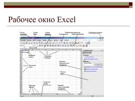
Рабочее окно Excel
Слайд 3

Создание таблицы
В клетки на рабочем листе Excel можно вводить:
Текст;
Формулы.
Формулы могут включать числа, ссылки на ячейки и диапазоны ячеек текущего рабочего листа или других листов, знаки математических действий
При создании таблицы используются приемы автозаполнения и автосуммирования.
Слайд 4

Пример таблицы
Слайд 5

Автоматизация при создании таблиц. Автозаполнение
Автозаполнение применяется если в строке или столбце содержатся:
Одни и те же числа или текст;
Числовой ряд (арифметическая или геометрическая прогрессия);
Стандартные списки (например, названия дней недели).
Слайд 6
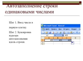
Автозаполнение строки одинаковыми числами
Шаг 1. Ввод числа в
первую клетку.
Шаг 2. Буксировка курсора автозаполнения вдоль строки.
Слайд 7
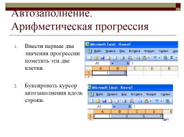
Автозаполнение. Арифметическая прогрессия
Ввести первые два значения прогрессии пометить эти две клетки.
Буксировать курсор автозаполнения вдоль строки.
Слайд 8

Автозаполнение. Геометрическая прогрессия
Заполнить первую клетку;
Пометить ряд клеток в строке или столбце, в которых должна быть прогрессия;
[Правка] — [Заполнить] — [Прогрессия…];
Выбрать тип прогрессии «геометрическая», задать шаг, конечное значение и щелкнуть левой кнопкой мыши на кнопке «OK» всплывающей панели «Прогрессия».
Слайд 9

Автосуммирование
Позволяет автоматически вычислять строку (столбец) с итоговыми суммами.
Слайд 10
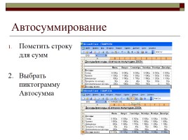
Автосуммирование
Пометить строку для сумм
2. Выбрать пиктограмму Автосумма
Слайд 11

Форматирование таблицы
Форматирование таблицы включает:
Форматирование ячеек;
Форматирование строк;
Форматирование таблицы в целом
Слайд 12
Форматирование ячеек
Для форматирования выбрать Format/Font
Форматирование ячеек включает задание:
Формата числа;
Выравнивание текста в ячейке;
Задание параметров шрифта;
Задание границ ячейки;
Заливку ячеек (цвет);
Введение защиты ячейки;
Слайд 13
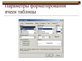
Параметры форматирования ячеек таблицы
Слайд 14
Условное форматирование ячеек таблицы
Можно задать особые параметры формата ячеек (например, другой цвет ячейки) в таблице при выполнении какого-либо условия (например, >100). Для этого:
Пометить ячейки таблицы;
[Формат]–[Условное форматирование…];
Задать условия и вид форматирования.
Слайд 15

Примечания к ячейкам
К любой ячейке таблицы можно создать примечание (комментарий). Для этого:
Пометить ячейку.
[Вставка] – [Примечание].
Ввести текст примечания.
Слайд 16

Форматирование строк/столбцов
Форматирование строк(столбцов) включает:
Настройку высоты строк (ширины столбцов);
Автоподбор высоты строк (ширины столбцов).
Слайд 17

Автоформат таблицы
При форматировании таблицы в целом выбирается один из стандартных видов внешнего оформления таблицы. Для этого:
Пометить форматируемую область таблицы;
[Формат] — [Автоформат] — [<Тип формата>].
Слайд 18
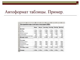
Автоформат таблицы. Пример.
Слайд 19
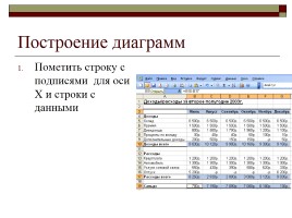
Построение диаграмм
Пометить строку с подписями для оси Х и строки с данными
Слайд 20
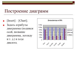
Построение диаграмм
[Insert] – [Chart];
Задать атрибуты диаграммы (подписи осей, название диаграммы, легенду и т. д.) в ходе диалога.
Слайд 21

Базы данных
Можно использовать таблицу как базу данных, так как в Excel предусмотрены средства сортировки и поиска данных в таблице по критериям, задаваемым пользователем, имеются средства интерфейса пользователя (формы) для работы с данными в таблицах.
Слайд 22
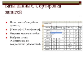
Базы данных. Сортировка записей
Пометить таблицу базы данных;
[Фильтр] – [Автофильтр];
Открыть меню в столбце;
Выбрать пункт «Сортировка по возрастанию (убыванию)»
Слайд 23
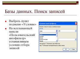
Базы данных. Поиск записей
Выбрать пункт подменю «Условие»
На всплывающей панели «Пользовательский автофильтр» устанавливаем условия отбора записей
Слайд 24

Анализ данных
Количество строк и столбцов таблицы и количество поставщиков или потребителей может быть очень велико (несколько сотен). Это затрудняет оценку итогов деятельности непосредственно по данным, приведенным в таблице.
Слайд 25

Анализ данных
В результате анализа часто требуется получить в сжатом виде данные по потребителям (фирмам):
Сколько каждой фирмой закуплено товаров за месяц по видам продукции;
Какая сумма фирмой уже выплачена;
Сколько фирма еще должна выплатить.
Слайд 26
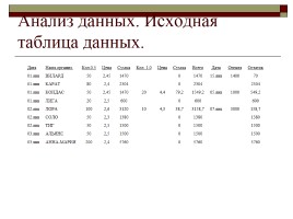
Анализ данных. Исходная таблица данных.
Слайд 27
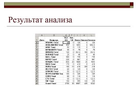
Результат анализа
Слайд 28

Создание сводной таблицы
Сводная таблица может включать результаты анализа сразу по двум показателям, например, содержать сводные данные о закупках или отгрузке продукции одновременно по фирмам и по датам.
Слайд 29
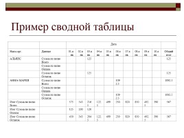
Пример сводной таблицы
Слайд 30

Решение задач. Подбор параметра.
Excel включает средства, позволяющие автоматически подбирать значения параметров, при которых достигается заданное значение какого-либо показателя, связанного функционально с этим параметром (например, достигать заданную прибыль при подборе значения накладных расходов)
Слайд 31
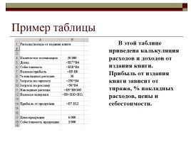
Пример таблицы
В этой таблице приведена калькуляция расходов и доходов от издания книги. Прибыль от издания книги зависит от тиража, % накладных расходов, цены и себестоимости.
Слайд 32
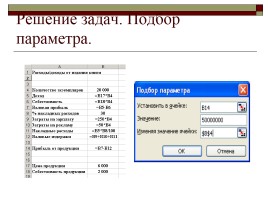
Решение задач. Подбор параметра.
Слайд 33

Решение задач. Подбор параметра
Пометить целевую ячейку;
[Сервис] – [Подбор параметра…];
В появившейся диалоговой панели «Подбор параметра» внести:
— в окно «Установить в ячейке:»- адрес целевой ячейки;
— в окно «Значение:» — желаемое значение в целевой ячейке;
— в окно «Изменяя значение ячейки:» — адрес изменяемой ячейки;
Слайд 34

Решение задачи оптимизации
В составе Excel есть программа Solver, предназначенная для нахождения значений нескольких параметров при наличии ограничений при которых значение параметра, связанного функционально с ними максимизируется или минимизируется. Примером может быть задача получения максимальной прибыли за счет перераспределения по кварталам затрат на рекламу.
Слайд 35

Решение задачи оптимизации
Слайд 36

Для решения задачи оптимизации нужно…
1. Пометить целевую ячейку;
2. [Сервис] — [Поиск решения…].
В результате появится диалоговая панель «Поиск решения»
Слайд 37
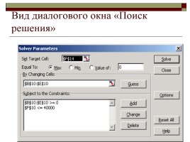
Вид диалогового окна «Поиск решения»
Слайд 38

В окнах диалоговой панели нужно задать…
— в окно «Установить целевую ячейку:» ввести адрес целевой ячейки:
— активизировать один из элементов (максимальному значению, минимальному значению) в группе «Равной:» или задать фиксированное значение, достигаемое в целевой ячейке в результате оптимизации в окно «значению»;
— указать диапазон изменяемых ячеек в окне «Изменяя ячейки:»;
— ввести ограничения в окно «Ограничения». Вызов панели ввода ограничений — щелчком левой кнопки мыши на кнопке «Добавить».
Слайд 39

Для получения автоотчета по результатам оптимизации нужно…
Во всплывающей после активизации кнопки Solver панели Solver Results нужно выбрать:
[Answer] – [OK]
Слайд 40

Создание и использование макросов
В макросы записывают последовательности команд, соответствующих выполнению нескольких часто повторяющихся последовательных действий с таблицами или диаграммами Excel. Запуск макроса будет приводить к автоматическому выполнению всей последовательности действий. Для возможности работы с макросами нужно установить низкий уровень защиты:
[Сервис] – [Макрос] – [Безопасность…] – [Низкая].
Слайд 41

Создание макроса с помощью макрорекордера
[Сервис] — [Макрос] — [Начать запись];
Вввести имя макроса в окно ввода “Имя макроса” панели “Запись макроса” и нажать кнопку [OK];
Выполнить действия с таблицей или диаграммой;
Остановить запись макроса щелчком левой кнопки мыши на кнопке “OK” всплывающей панели «Остановить запись макроса».
Слайд 42

Запуск макроса
[Сервис] — [Макрос] – [Макросы…] ;
Выбрать из меню нужный макрос;
[Выполнить].
Слайд 43

Создание средств запуска макросов
Для запуска макросов могут быть созданы и использоваться:
кнопки, которые могут быть добавлены в имеющиеся пиктографические меню Excel;
кнопки управления “Кнопка” из панели инструментов “Формы”;
графические объекты и объекты WordArt.
Слайд 44

Для создания кнопки в пиктографическом меню нужно…
[Вид] — [Панели инструментов] — [Настройка…];
[Команды] – [Макросы];
Отбуксировать кнопку “Кнопка” на имеющуюся панель инструментов, например, на панель “Стандартная”;
[Закрыть].
Слайд 45

Для создания кнопки управления на рабочем листе нужно…
[Вид] – [Панели инструментов] – [Формы];
Выбрать объект “Кнопка” и установить его в нужном месте листа рабочей книги Excel и нужного размера;
Связать кнопку “Кнопка” с макросом для чего вызвать контекстное меню правой кнопкой мыши и выбрать пункт “Назначить макрос”, затем указать требуемый макрос в списке.
Слайд 46

Для создания средства запуска макроса в форме графического объекта или объекта WordArt нужно…
Создать такой объект;
Вызвать контекстное меню правой кнопкой мыши и выбрать пункт “Назначить макрос”, затем указать требуемый макрос в списке.