
Excel for Microsoft 365 Excel for Microsoft 365 for Mac Excel for the web Excel 2021 Excel 2021 for Mac Excel 2019 Excel 2019 for Mac Excel 2016 Excel 2016 for Mac Excel 2013 Excel 2010 Excel 2007 Excel for Mac 2011 Excel Starter 2010 More…Less
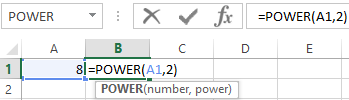
Let’s say you want to calculate an extremely small tolerance level for a machined part or the vast distance between two galaxies. To raise a number to a power, use the POWER function.
Description
Returns the result of a number raised to a power.
Syntax
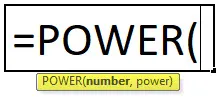
POWER(number, power)
The POWER function syntax has the following arguments:
-
Number Required. The base number. It can be any real number.
-
Power Required. The exponent to which the base number is raised.
Remark
The «^» operator can be used instead of POWER to indicate to what power the base number is to be raised, such as in 5^2.
Example
Copy the example data in the following table, and paste it in cell A1 of a new Excel worksheet. For formulas to show results, select them, press F2, and then press Enter. If you need to, you can adjust the column widths to see all the data.
|
Formula |
Description |
R |
|
=POWER(5,2) |
5 squared. |
25 |
|
=POWER(98.6,3.2) |
98.6 raised to the power of 3.2. |
2401077.222 |
|
=POWER(4,5/4) |
4 raised to the power of 5/4. |
5.656854249 |
Need more help?
Want more options?
Explore subscription benefits, browse training courses, learn how to secure your device, and more.
Communities help you ask and answer questions, give feedback, and hear from experts with rich knowledge.
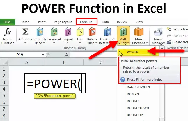
In mathematics, we had exponents, the power to a given base number. In Excel, we have a similar built-in function known as the POWER function, which is used to calculate the power of a given number or base. To use this function, we can use the keyword =POWER( in a cell and provide two arguments, one as the number and another as power.
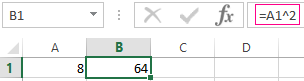
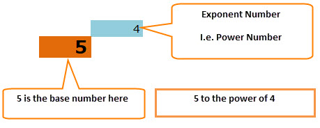
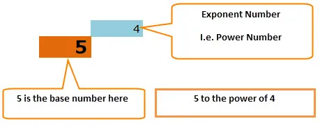
For example, suppose the base number 4 is raised to the power number 3. i.e., 4 cube. =4*4*4 = 64.
A POWER in Excel is a Math/Trigonometric function that computes and returns the result of a number raised to a power. The POWER Excel function takes two arguments: the base (any real number) and the exponent (power that signifies how many times the given number will be multiplied by itself). For example, 5 multiplied by a power of 2 is the same as 5 x5.
Table of contents
- Power in Excel
- Formula of POWER Function
- Explanation of POWER Function in Excel
- How to Use POWER Function in Excel
- POWER in Excel Example #1
- POWER in Excel Example #2
- POWER in Excel Example #3
- POWER in Excel Example #4
- Recommended Articles
The Formula of POWER Function


Explanation of POWER Function in Excel
The POWER function in Excel takes both arguments as a numeric value. Hence, the arguments passed are of integer type where the number is the base number, and the POWER is the exponent. Both arguments are required and are not optional.


We can use the POWER function in Excel in many ways, like for mathematical operations. For example, we can use the POWER function equation to compute the relational algebraic functions.
How to Use POWER Function in Excel
The Excel POWER function is very simple and easy to use. Let us understand the working of POWER in Excel by some examples.
You can download this POWER Function Excel Template here – POWER Function Excel Template
POWER in Excel Example #1
We have a POWER function equation y=x^n (x to the power n), where y is dependent on the value of x, and n is the exponent. We also want to draw the graph of this f(x, y) function for given values of x and n=2. For example, the values of x are:

So, in this case, since the value of y depends upon the nth power of x, we will calculate the value of Y using the POWER function in Excel.
- 1st value of y will be 2^2 (=POWER(2,2)
- 2nd value of y will be 4^2 (=POWER(4,2)
- ……………………………………………………………
- ……………………………………………………………
- 10th value of y will be 10^2 (=POWER(10,2)

Now, selecting the values of x and y from range B4:K5, choose the graph (in this example, we have chosen the scatter graph with smooth lines) from the “Insert” tab.

So, we get a linear, exponential graph for the given POWER function equation.

POWER in Excel Example #2
In algebra, we have the quadratic POWER function equation, represented as ax2+bx+c=0, where x is unknown, and a, b and c are the coefficients. The solution of this POWER function equation gives the roots of the equation, which are the values of x.
The roots of the quadratic POWER function equation are computed by following mathematical formula:
- x = (-b+ (b2-4ac)1/2)/2a
- x = (-b- (b2-4ac)1/2)/2a
b2-4ac is called discriminant and describes a quadratic POWER function equation’s number of roots.
Now, we have a list of quadratic POWER function equations given in column A. But, first, we need to find the roots of the equations.

^ is the exponential operator used to represent the power (exponent). For example, X2 is the same as x^2.
We have five quadratic POWER function equations, and we will solve them using the formula with the help of the POWER function in Excel to find the roots.
In the first POWER function equation, a=4, b=56, and c = -96. If we mathematically solve them using the above formula, we have the roots -15.5 and 1.5.

To implement this in Excel formula, we will use the POWER function in Excel and the formula will be:
- =((-56+POWER(POWER(56,2)-(4*4*(-93)),1/2)))/(2*4) will give the first root and
- =((-56-POWER(POWER(56,2)-(4*4*(-93)),1/2)))/(2*4) will give the second root of the equation
So, the complete formula will be,
=”Roots of equations are”&” “&((-56+POWER(POWER(56,2)-(4*4*(-93)),1/2)))/(2*4)&” , “&((-56-POWER(POWER(56,2)-(4*4*(-93)),1/2)))/(2*4)
The formulas are concatenated with the string “Roots of equation are.”
Using the same formula for other POWER function equations, we have:

Output:

POWER in Excel Example #3
So, we can use the POWER function in Excel for different mathematical calculations.
Suppose we have to find out the compound interestCompound interest is the interest charged on the sum of the principal amount and the total interest amassed on it so far. It plays a crucial role in generating higher rewards from an investment.read more for which the formula is:
Amount = Principal (1 + r/n)nt
- Where r is the interest rate, n is the number of times interest is compounded per year, and t is the time.
- If an amount of $4,000 is deposited into an account (saving) at an interest rate of 5% annually, compounded monthly, the value of the investment after 5 years can be calculated using the above compound interest formula.
- When, Principal = $4000, rate = 5/100 that is 0.05, n =12 (compounded monthly), time =5 years.
We have the formula using the compound interest formula and implementing it into the Excel formula using the POWER function.
=B2*(POWER((1+(B3/B5)),(B4*B5)))
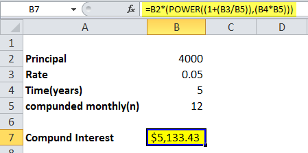
So, the investment balance after 5 years is $5.133.43.
POWER in Excel Example #4
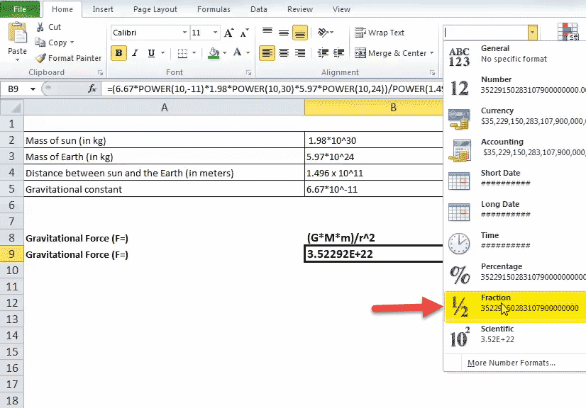
According to Newton’s gravitation law, two bodies at a distance of r from their center of gravity attract each other in the universe according to a gravitational POWER Excel formula.
F = (G*M*m)/r2
When F is the magnitude of the gravitational force, G is called the gravitational constant, M is the mass of the first body, m is the mass of the second body, and r is the distance between the bodies from their center of gravity.
Let us calculate the magnitude of gravitational force by which the sun pulls the earth.
- The mass of the sun is 1.98*10^30 kg.
- The mass of the earth is 5.97*10^24 kg.
- The distance between the sun and the earth is 1.496 x 10^11 meters.
- Gravitational constant value is 6.67*10^-11 m3kg-1s-2.
In Excel, if we want to calculate the gravitational force, we will again be using the POWER in Excel that can operate over big numeric values.
- So, we can convert the scientific notation values into the POWER Excel formula using the POWER in Excel.
- 1.98*10^30 will be represented as 1.98*Power(10,30), similarly to other values.
- So, the POWER Excel formula to calculate the force will be: = (6.67*POWER(10,-11)*1.98*POWER(10,30)*5.97*POWER(10,24))/POWER(1.496*POWER(10,11),2)

Since the value obtained as force is a big number Excel expressed it scientific notationIn Excel, scientific notation is a specific style of writing numbers in scientific and exponential forms. Scientific notation compactly helps display values, allowing us to compare and use the same in calculations.read more. To change it into a fraction, change the format to the fraction.
Output:
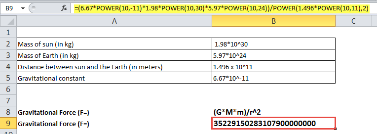
So, the sun pulls the earth with a force of magnitude 35229150283107900000000 Newton.
Recommended Articles
This article is a guide to the POWER Function in Excel. Here, we discuss the POWER formula in Excel and how to use the POWER Excel function, along with Excel examples and downloadable Excel templates. You may also look at these useful functions in Excel: –
- Excel vs. AccessExcel and Access are two of Microsoft’s most powerful tools for data analysis and report generation, but there are some significant differences between them. Excel is an older product of Microsoft, whereas Access is the most advanced and complex product of Microsoft. Excel is very easy to create dashboards and formulas, whereas Access is very easy for databases and connections.read more
- GetPivotData in Excel
- NOT Function
Содержание
- POWER в Excel (формула, примеры) — Как использовать функцию POWER?
- СИЛА в Excel
- POWER Formula в Excel
- Как использовать функцию POWER в Excel?
- Пример № 1
- Пример № 2
- Пример № 3
- Функция POWER в VBA
- Что нужно помнить о функции POWER
- Рекомендуемые статьи
- How to raise a number to a power in Excel using the formula and operator
- How to raise to the power of in excel?
- Variant 1. Use the character «^»
- Variant 2. Using the function
- Formula for the exponentiation in Excel
- Square root power in Excel
- How to write a number to the degree in Excel?
POWER в Excel (формула, примеры) — Как использовать функцию POWER?

ВЛАСТЬ в Excel (Содержание)
- СИЛА в Excel
- POWER Formula в Excel
- Как использовать функцию POWER в Excel?
СИЛА в Excel
Я до сих пор помню дни, когда мой учитель математики почти каждый день бил меня за то, что я не помнил КВАДРАТНЫЙ КОРЕНЬ чисел. Я буквально плакал, когда наступил математический период. Есть много случаев, когда я занимался математикой только для того, чтобы избежать побоев со стороны моего учителя математики.
Хорошо, теперь мне не нужно запоминать все эти КВАДРАТНЫЕ КОРНИ, вместо этого я могу положиться на красивую функцию под названием POWER Function.
Функция POWER помогает поднять число в другое число раз до мощности.
Например: каково значение 5 на квадрат 3? Ответ 5 * 5 * 5 = 125 .
POWER Formula в Excel
Ниже приведена формула СИЛА:

Функция Power включает в себя два параметра, и оба являются обязательными аргументами.
Число: число, которое вам нужно для поднятия силы, т.е. базовое число любого действительного числа.
Мощность: сколько раз вам нужно поднять базовое число. Это показатель для поднятия базового числа.
Символ или оператор (оператор каретки) действует как показатель степени. Например: 6 2 = 36. Это не 6 умножается на 2, а 6 * 6 = 36. Шесть умножается на сам шесть дважды.

Простое уравнение 5 * 5 * 5 * 5 = 625
Как использовать функцию POWER в Excel?
Эта функция POWER очень проста в использовании. Давайте теперь посмотрим, как использовать функцию POWER с помощью нескольких примеров.
Вы можете скачать эту функцию POWER в шаблоне Excel здесь — функция POWER в шаблоне Excel
Пример № 1
Предположим, у вас есть базовые числа из A2: A6 и степенное число (экспоненциальные числа) из B2: B6. Показать мощность значений в столбце A, используя числа питания в столбце B.

Применить формулу силы в ячейке C2


Перетащите формулу в другие ячейки.

- Первое значение — это базовое число 8, возведенное в степень 3, то есть 8 куб. = 8 * 8 * 8 = 512.
Во-вторых, базовое число 11 повышается до степени 6, то есть 11 умножается в 6 раз на 11. = 11 * 11 * 11 * 11 * 11 * 11 = 17, 71 561. Точно так же все значения привели таким образом.
Пример № 2
Используйте те же данные из приведенного выше примера. Вместо использования функции POWER мы используем оператор каретки (^) для выполнения расчетов. Результаты будут такими же, хотя.

Примените формулу в ячейке H2


Перетащите формулу в другие ячейки.

Пример № 3
Использование функции POWER вместе с другими функциями. Из приведенных ниже данных увеличьте все четные числа на 2, если число не четное, то увеличьте значение на 5.
Здесь сначала нужно проверить, является ли число четным или нет. Если число найдено даже тогда, увеличьте мощность на 2, если не увеличьте мощность на 5.

Проблема такого типа может быть решена с помощью условия IF, чтобы проверить, является ли число четным или нет.
Примените формулу в ячейке B2.


Перетащите формулу в другие ячейки.

- Если условие IF проверяет, равно ли указанное число четному числу или нет. = ЕСЛИ (А2 = РАВ (А2),
- Если логика ПЧ истинна, функция POWER повысит мощность на 2. = POWER (A2, 2),
- Если логика ПЧ ложна, функция POWER увеличивает мощность на 5. = POWER (A2, 5),
Функция POWER в VBA
В VBA также мы можем использовать функцию POWER. Однако дело в том, что мы не видим многих из этих живых примеров в нашей повседневной жизни.
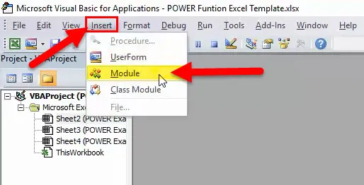
Шаг 1: Откройте редактор VBA (ALT + F11).

Шаг 2: Перейти, чтобы вставить и вставить модуль. Это мгновенно создаст новый модуль для написания нашего кода для функции POWER

Шаг 3: Скопируйте и вставьте приведенный ниже код в новый модуль.
Dim My_Result As String
My_Result = Application.WorksheetFunction.Power (6, 3)
Теперь ваше окно должно выглядеть так, как показано ниже.

Если вы запустите код, вы получите следующий результат.

Что нужно помнить о функции POWER
- Для лучшего понимания мы можем представить степенную функцию таким образом. POWER (X, Y) или POWER (X Y) оба одинаковы.
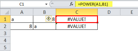
- Функция POWER применяется только для числовых значений. Что-нибудь кроме числовых значений, это вызовет ошибку как # ЗНАЧЕНИЕ! Если какой-либо из параметров содержит нечисловые значения, мы получим ошибку. На рисунке ниже показан пример ошибки.

Это покажет ошибку.

Рекомендуемые статьи
Это было руководство к функции питания. Здесь мы обсуждаем формулу POWER и как использовать функцию POWER вместе с практическими примерами и загружаемыми шаблонами Excel. Вы также можете просмотреть наши другие предлагаемые статьи —
- Как использовать функцию поиска в Excel?
- Функция Excel НЕ
- ТРАНСПОЗИРОВАТЬ функцию Excel
- LOOKUP в MS Excel
Источник
How to raise a number to a power in Excel using the formula and operator
Often, users need to raise a number to a power. How to do it correctly with the help of «Excel»?
In this article, we will try to understand popular user questions and give instructions on how to use the system correctly. MS Office Excel allows you to perform a number of mathematical functions: from the simplest to the most complex. This universal software is designed for all occasions.
How to raise to the power of in excel?
Before searching for the required function, pay attention to the mathematical laws:
- «1» will remain «1» to any degree.
- «0» will remain «0» to any degree.
- Any number raised to zero degree equals one.
- Any value of «A» in the power of «1» will be equal to «A».
Examples in Excel:
Variant 1. Use the character «^»
The standard and easiest option is to use the «^» icon, which is obtained by pressing Shift + 6 with the English keyboard layout.
- In order for the number to be exponentiation to the required degree, it is necessary to put the «=» sign in the cell before specifying the number you want to build.
- The degree is indicated after the sign «^».
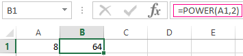
We built 8 into a «square» (that is, to the second degree) and got the result of the calculation in cell «A2».
Variant 2. Using the function
In Microsoft Office Excel there is a convenient function «POWER», which you can activate for simple and complex mathematical calculations
The function looks like this:
- The numbers for this formula are indicated without spaces or other signs.
- The first digit is the value «number». This is the basis (that is, the figure that we are building). Microsoft Office Excel allows the introduction of any real number.
- The second figure is the value of «degree». This is an indicator in which we build the first figure.
- The values of both parameters can be less than zero ( with a «-» sign).
Formula for the exponentiation in Excel
Examples of using the =POWER() function.
Using the function wizard:
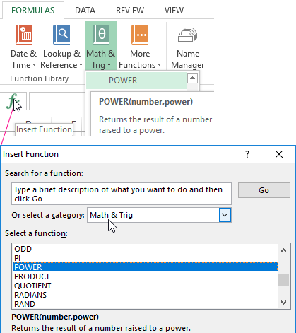
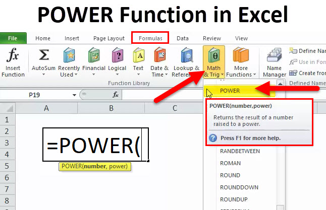
- Start the function wizard by using the hotkey combination SHIFT + F3 or click on the button at the beginning of the formula line «fx» (insert function). From the «Or select a category:» drop-down list, select «Math & Trig», and in the bottom field «Select a function:», specify the function «POWER» we need and click OK. Or select: «FORMULAS»-«Function Library»-«Math & Trig»-«POWER».

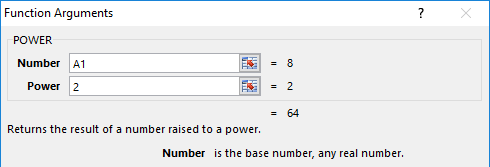
- In the dialog that appears, fill in the fields with arguments. For example, we need to exponentiate «2» to the degree of «3». Then in the first field enter «2», and in the second — «3».
- Press the «OK» button and get in the cell into which the formula was entered, the value we need. For this situation, it is «2» in the «cube», i.e. 2 * 2 * 2 = 8. The program has calculated everything correctly and has given you the result.
If you think that extra clicks are a dubious pleasure, we offer one simpler variant.
Entering the function manually:
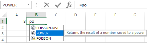
- In the formula line we put the sign «=» and begin to enter the name of the function. Usually it is enough to write «=po…» — and the system itself will guess to offer you a useful option.
- As soon as you saw such a hint, just press the «Tab» key. Or you can continue to write, manually enter each letter. Then in parentheses, specify the required parameters: two numbers separated by a semicolon.
- After that, click on «Enter» — and in the cell the calculated value 8 appears.
The sequence of actions is simple, and the user gets the result quickly enough. In arguments, instead of numbers, you can specify cell references.
Square root power in Excel
To extract the root using Microsoft Excel formulas, we use a slightly different, but very convenient, way of calling functions:
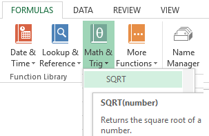
- Go to the «FORMULAS» tab. In the «Function Library» section of the toolbar, click on the «Math & Trig» tool. And from the drop-down list, select the «SQRT» option.
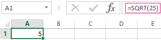
- Enter the function argument at the system request. In our case, it was necessary to find the root from «25», so we enter it into the line. After entering the number, just click on the «OK» button. In the cell, the figure obtained as a result of the mathematical calculation of the root will be reflected.
ATTENTION! If we need to know the root of the degree in Excel then we do not use the function =SQRT(). Let us recall the theory from mathematics:
«A root of the n -th degree of a is a number b whose n -th degree is equal to a «, that is:
n √a = b; b n = a
«A root of n -th degree from the number a will be equal to raising to the degree of the same number a by 1/ n «, that is:
n √a = a 1/n
From this it follows that to calculate the mathematical formula of the root in the n -th degree for example:
5 √32 = 2
In Excel, you should write through this formula: = 32 ^ (1/5), that is: = a ^ (1 / n) — where a is a number; N-degree:
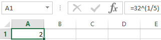
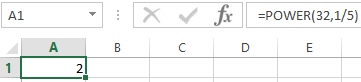
Or through this function: =POWER(32,1/5)
In the arguments of a formula and a function, you can specify cell references instead of the numbers.
How to write a number to the degree in Excel?
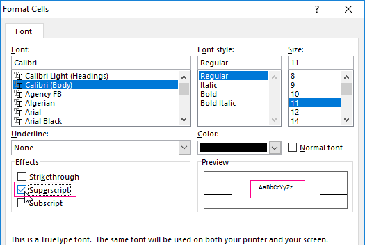
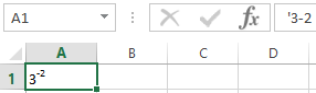
It is often important for you that the number in the degree is correctly displayed when printing and looks beautiful in the table. How to write a number to the degree in Excel? Here you need to use the Format Cells tab. In our example, we recorded «3» in the cell «A1», which should be presented to the -2 degree.
The sequence of actions is as follows:
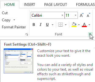
- Right click on the cell with the number and select the tab «Format Cells» from the pop-up menu. If it does not work out — find the «Format Cells» tab in the top panel or press CTRL + 1.
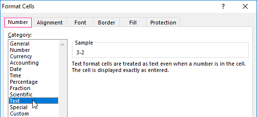
- In the menu that appears, select the «Number» tab and set the format for the «Text» cell. Click OK.
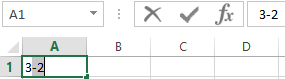
- In cell A1 enter «-2» next to «3» and select it.
- Again, we call the format of cells (for example, by pressing CTRL + 1 hot keys) and now the «Font» tab is only available for us, where we tick the «Superscript» option. And click OK.
- The result should display the following meaning:
Using Excel’s features is easy and convenient. With them you save time on the implementation of mathematical calculations and the search for the necessary formulas.
Источник
Summary
The Excel POWER function returns a number raised to a given power. The POWER function is an alternative to the exponent operator (^).
Purpose
Raise a number to a power
Return value
Arguments
- number — Number to raise to a power.
- power — Power to raise number to (the exponent).
Syntax
Usage notes
The POWER function returns a number raised to a given power. POWER is an alternative to the exponent operator (^) in a math equation.
The POWER function takes two arguments: number and power. Number should be a numeric value, provided as a hardcoded constant or as a cell reference. The power argument functions as the exponent, indicating the power to which number should be raised.
Examples
To raise 2 to the 3rd power, you can use POWER like this:
=POWER(2,3) // returns 8
To raise 2 to the 8th power:
=POWER(2,8) // returns 256
To cube the value in cell A1:
=POWER(A1,3) // cube A1
Fractional exponents
To use the power function with a fractional exponent, enter the fraction directly as the power argument:
=POWER(27,1/3) // returns 3
=POWER(81,1/4) // returns 3
=POWER(256,1/8) // returns 2
Exponent operator
In Excel, exponentiation can also be handled with the exponent (^) operator, so:
=2^2=POWER(2,2)=4
=2^3=POWER(2,3)=8
=2^4=POWER(2,4)=16

Author![]()
Dave Bruns
Hi — I’m Dave Bruns, and I run Exceljet with my wife, Lisa. Our goal is to help you work faster in Excel. We create short videos, and clear examples of formulas, functions, pivot tables, conditional formatting, and charts.
This is the best learning resource I have stumbled upon in many years during the process of my Excel learning.
Get Training
Quick, clean, and to the point training
Learn Excel with high quality video training. Our videos are quick, clean, and to the point, so you can learn Excel in less time, and easily review key topics when needed. Each video comes with its own practice worksheet.
View Paid Training & Bundles
Help us improve Exceljet
POWER in Excel (Table of Contents)
- POWER in Excel
- POWER Formula in Excel
- How to Use POWER Function in Excel?
POWER in Excel
I still remember the days when my maths teacher beat me almost every day for not remembering the SQUARE ROOT of numbers. I literally cried when maths period is on the way. There are many instances where I bunked the math class just to get away from those beatings from my maths teacher.
Ok, now I need not to remember all those SQUARE ROOTS; instead, I can rely on a beautiful function called the POWER Function.
POWER function helps in raising the number to another number of times to the power.
For example: What is the value of 5 to the square of 3? The answer is 5*5*5 = 125.
POWER Formula in Excel
Below is the POWER Formula:
The Power Function includes two parameters, and both are required arguments.
- Number: The number you need to raise the power, i.e. the base number of any real number.
- Power: The number of times you need to raise the base number. It is the exponent to raise the base number.
The symbol or operator ^ (caret operator) acts as an exponent. For example: 6^2 = 36. This is not 6 is multiplied by 2 rather 6 * 6 = 36. Six is multiplied by the six itself twice.
The simple equation is 5 * 5 * 5 * 5 = 625
How to Use the POWER Function in Excel?
This POWER function is very simple easy to use. Let us now see how to use the POWER Function with the help of some examples.
You can download this POWER Function in Excel Template here – POWER Function in Excel Template
Example #1
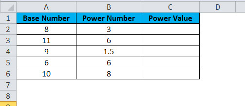
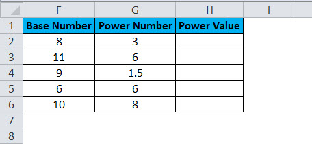
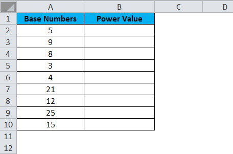
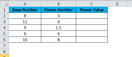
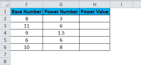
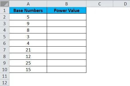
Assume you have base numbers from A2:A6 and the power number (exponential numbers) from B2:B6. Show the power of values in column A by using power numbers in column B.
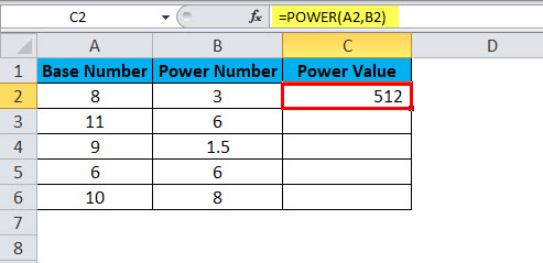
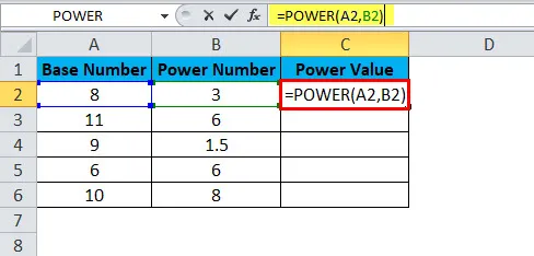
Apply Power formula in the cell C2

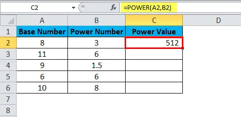
The answer will be:
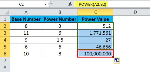
Drag and drop the formula to other cells.
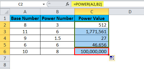
- The first value is base number 8 is raised to the power number 3. i.e. 8 cube. =8*8*8 = 512.
Secondly, base number 11 is raised to the power number 6, i.e. 11 is multiplied 6 times to the 11 itself. =11 * 11* 11* 11* 11* 11 = 17, 71,561. Similarly, all the values have resulted in that way.
Example #2
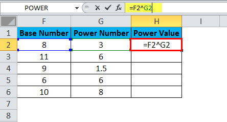
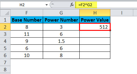
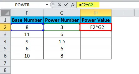
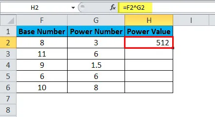
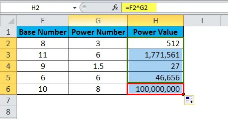
Use the same data from the above example. Instead of using the POWER Function, we use the caret operator (^) to do the calculation. The results will be the same, though.
Apply formula in the cell H2
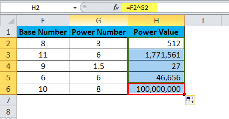
The answer will be:
Drag and drop the formula to other cells.
Example #3
Using POWER Function along with other functions. From the below data, raise all the even numbers power by 2; if the number is not even, then raise the power by 5.
Here, first, we need to test whether the number is even or not. If the number found, raise the power by 2; if not, raise the power by 5.
This type of problem can be addressed by using the IF condition to test whether the number is even or not.
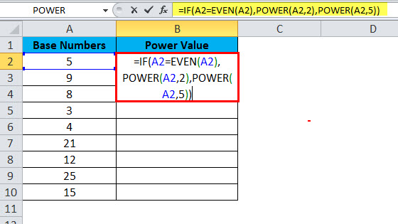
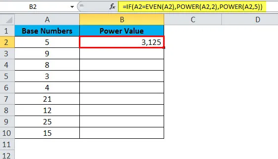
Apply formula in cell B2.
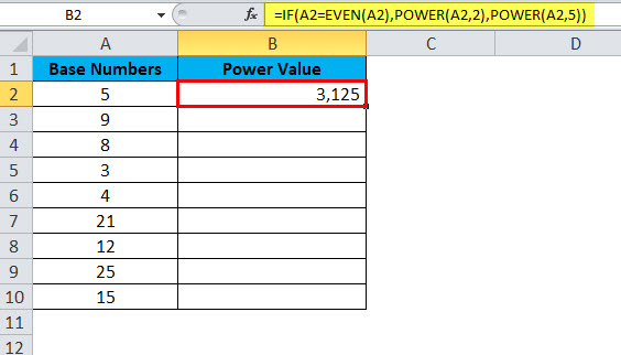
The answer will be:
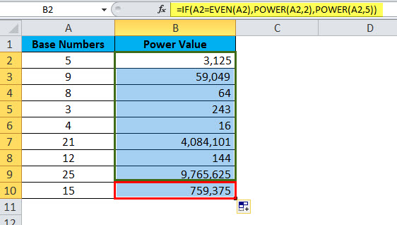
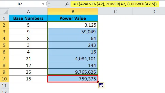
Drag and drop the formula to other cells.
- IF condition tests whether the supplied number is equal to an even number or not. =IF(A2=EVEN(A2),
- If the IF logic is true then the POWER function will raise the power by 2. =POWER(A2,2),
- If the IF logic is false, then the POWER function will raise the power by 5. =POWER(A2,5),
POWER Function in VBA
In VBA, also we can use the POWER function. However, the thing is, we do not get to see many of these live examples in our day-to-day life.
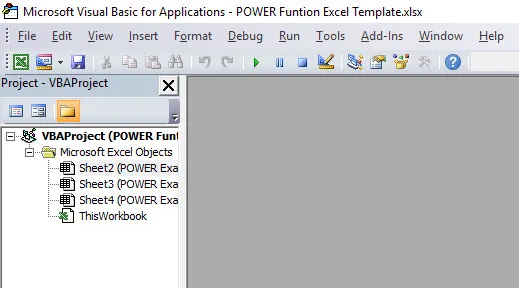
Step 1: Open your VBA editor (ALT + F11).
Step 2: Go to insert and insert Module. This would instantly create a new module to write our code for the POWER function.

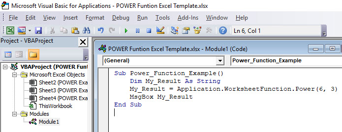
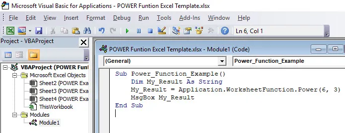
Step 3: Copy and paste the below code inside the new module.
Sub Power_Function_Example ()

Dim My_Result As String

My_Result = Application.WorksheetFunction.Power(6, 3)

MsgBox My_Result

End Sub
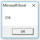
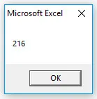
Now your window should look like the one below one.
If you run the code, you will get the below result.
Things to Remember about POWER Function
- For a better understanding, we can represent the power function in this way. POWER(X, Y) or POWER(X^Y) both are the same only.
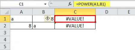
- The POWER function is applied only for numerical values. Anything other than numerical values, it will throw the error as #VALUE! If any one of the parameters contains non-numerical values, we will get the error. The below image shows an example of the error.
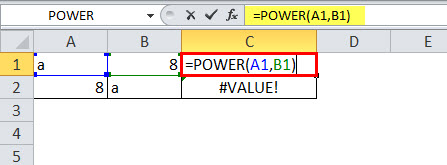
It will show an error.
Recommended Articles
This has been a guide to POWER Function. Here we discuss the POWER Formula and how to use the POWER Function along with practical examples and downloadable excel templates. You can also go through our other suggested articles –
- How to Use FIND Function in Excel?
- Excel NOT Function
- TRANSPOSE Excel Function
- LOOKUP in MS Excel
- СИЛА в Excel

ВЛАСТЬ в Excel (Содержание)
- СИЛА в Excel
- POWER Formula в Excel
- Как использовать функцию POWER в Excel?
СИЛА в Excel
Я до сих пор помню дни, когда мой учитель математики почти каждый день бил меня за то, что я не помнил КВАДРАТНЫЙ КОРЕНЬ чисел. Я буквально плакал, когда наступил математический период. Есть много случаев, когда я занимался математикой только для того, чтобы избежать побоев со стороны моего учителя математики.
Хорошо, теперь мне не нужно запоминать все эти КВАДРАТНЫЕ КОРНИ, вместо этого я могу положиться на красивую функцию под названием POWER Function.
Функция POWER помогает поднять число в другое число раз до мощности.
Например: каково значение 5 на квадрат 3? Ответ 5 * 5 * 5 = 125 .
POWER Formula в Excel
Ниже приведена формула СИЛА:
Функция Power включает в себя два параметра, и оба являются обязательными аргументами.
Число: число, которое вам нужно для поднятия силы, т.е. базовое число любого действительного числа.
Мощность: сколько раз вам нужно поднять базовое число. Это показатель для поднятия базового числа.
Символ или оператор (оператор каретки) действует как показатель степени. Например: 6 2 = 36. Это не 6 умножается на 2, а 6 * 6 = 36. Шесть умножается на сам шесть дважды.
Простое уравнение 5 * 5 * 5 * 5 = 625
Как использовать функцию POWER в Excel?
Эта функция POWER очень проста в использовании. Давайте теперь посмотрим, как использовать функцию POWER с помощью нескольких примеров.
Вы можете скачать эту функцию POWER в шаблоне Excel здесь — функция POWER в шаблоне Excel
Пример № 1
Предположим, у вас есть базовые числа из A2: A6 и степенное число (экспоненциальные числа) из B2: B6. Показать мощность значений в столбце A, используя числа питания в столбце B.
Применить формулу силы в ячейке C2
Ответ будет:
Перетащите формулу в другие ячейки.
- Первое значение — это базовое число 8, возведенное в степень 3, то есть 8 куб. = 8 * 8 * 8 = 512.
Во-вторых, базовое число 11 повышается до степени 6, то есть 11 умножается в 6 раз на 11. = 11 * 11 * 11 * 11 * 11 * 11 = 17, 71 561. Точно так же все значения привели таким образом.
Пример № 2
Используйте те же данные из приведенного выше примера. Вместо использования функции POWER мы используем оператор каретки (^) для выполнения расчетов. Результаты будут такими же, хотя.
Примените формулу в ячейке H2
Ответ будет:
Перетащите формулу в другие ячейки.
Пример № 3
Использование функции POWER вместе с другими функциями. Из приведенных ниже данных увеличьте все четные числа на 2, если число не четное, то увеличьте значение на 5.
Здесь сначала нужно проверить, является ли число четным или нет. Если число найдено даже тогда, увеличьте мощность на 2, если не увеличьте мощность на 5.
Проблема такого типа может быть решена с помощью условия IF, чтобы проверить, является ли число четным или нет.
Примените формулу в ячейке B2.

Ответ будет:
Перетащите формулу в другие ячейки.
- Если условие IF проверяет, равно ли указанное число четному числу или нет. = ЕСЛИ (А2 = РАВ (А2),
- Если логика ПЧ истинна, функция POWER повысит мощность на 2. = POWER (A2, 2),
- Если логика ПЧ ложна, функция POWER увеличивает мощность на 5. = POWER (A2, 5),
Функция POWER в VBA
В VBA также мы можем использовать функцию POWER. Однако дело в том, что мы не видим многих из этих живых примеров в нашей повседневной жизни.
Шаг 1: Откройте редактор VBA (ALT + F11).
Шаг 2: Перейти, чтобы вставить и вставить модуль. Это мгновенно создаст новый модуль для написания нашего кода для функции POWER
Шаг 3: Скопируйте и вставьте приведенный ниже код в новый модуль.
Sub Power_Function_Example ()
Dim My_Result As String
My_Result = Application.WorksheetFunction.Power (6, 3)
MsgBox My_Result
End Sub
Теперь ваше окно должно выглядеть так, как показано ниже.
Если вы запустите код, вы получите следующий результат.
Что нужно помнить о функции POWER
- Для лучшего понимания мы можем представить степенную функцию таким образом. POWER (X, Y) или POWER (X Y) оба одинаковы.
- Функция POWER применяется только для числовых значений. Что-нибудь кроме числовых значений, это вызовет ошибку как # ЗНАЧЕНИЕ! Если какой-либо из параметров содержит нечисловые значения, мы получим ошибку. На рисунке ниже показан пример ошибки.

Это покажет ошибку.
Рекомендуемые статьи
Это было руководство к функции питания. Здесь мы обсуждаем формулу POWER и как использовать функцию POWER вместе с практическими примерами и загружаемыми шаблонами Excel. Вы также можете просмотреть наши другие предлагаемые статьи —
- Как использовать функцию поиска в Excel?
- Функция Excel НЕ
- ТРАНСПОЗИРОВАТЬ функцию Excel
- LOOKUP в MS Excel

This Excel tutorial explains how to use the Excel POWER function with syntax and examples.
Description
The Microsoft Excel POWER function returns the result of a number raised to a given power.
The POWER function is a built-in function in Excel that is categorized as a Math/Trig Function. It can be used as a worksheet function (WS) in Excel. As a worksheet function, the POWER function can be entered as part of a formula in a cell of a worksheet.
Syntax
The syntax for the POWER function in Microsoft Excel is:
POWER( number, power )
Parameters or Arguments
- number
- It is the base number.
- power
- It is the exponent used to raise the base number to.
Returns
The POWER function returns a numeric value.
Applies To
- Excel for Office 365, Excel 2019, Excel 2016, Excel 2013, Excel 2011 for Mac, Excel 2010, Excel 2007, Excel 2003, Excel XP, Excel 2000
Type of Function
- Worksheet function (WS)
Example (as Worksheet Function)
Let’s look at some Excel POWER function examples and explore how to use the POWER function as a worksheet function in Microsoft Excel:
Based on the Excel spreadsheet above, the following POWER examples would return:
=POWER(A1, A2)
Result: 81

=POWER(A1, A3)
Result: 140.2961154

=POWER(A2, 2)
Result: 16
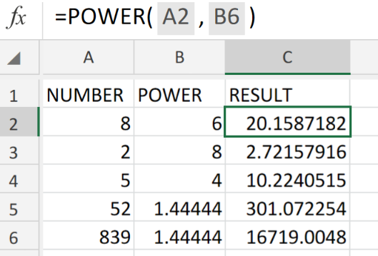 Figure 1. of Excel POWER Function.
In the event that we want to determine a very small level of tolerance for vast distances. At some point we will have to raise a number to a specific power. We are going to utilize the Excel POWER Function. This article will walk through how to do it.
Generic Formula
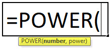
POWER(number, power)
The POWER Function will calculate a number raised to a specific power. The formula syntax has the following components;
- number – the number value which we desire to raise to a certain power. This can be any real number.
- power – the exponential value to which we are going to raise our base number.
How to use the Excel POWER Function.
We can achieve this by following three simple steps!
- Collect the data available to us for checking, in our Excel sheet. See example illustrated below;
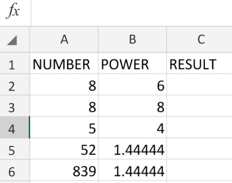 Figure 2. of Number Values for the POWER Function in Excel.
- Our purpose here is to exponentially raise the number values in column A to the power Values specified in column B of our worksheet. The formula syntax which we will enter into the formula bar for cell C2, for the desired result is as follows;
=POWER(A2,B6)
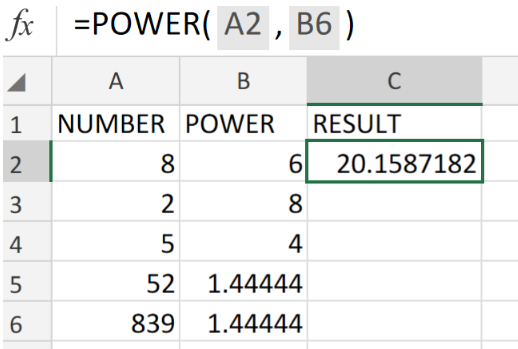 Figure 3. of the POWER Function in Excel.
- Modify and copy the formula syntax into the other cells in column C of the example illustrated below to achieve the desired results.
 Figure 4. of the POWER Function in Excel.
The POWER Function operates like an exponential value in a basic mathematical equation.
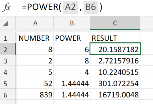 Figure 5. of Final Result.
Instant Connection to an Expert through our Excelchat Service
Our live Excelchat Service is here for you. We have Excel Experts available 24/7 to answer any Excel questions you may have. Guaranteed connection within 30 seconds and a customized solution for you within 20 minutes.
Did this post not answer your question? Get a
solution from
connecting
with the expert.
Another blog reader asked this question today on Excelchat:

what is 2 to the 431 power. what is 3 to 421 power
An Excelchat Expert solved this problem in 24 mins!