Power to function excel - Word и Excel - помощь в работе с программами

Excel for Microsoft 365 Excel for Microsoft 365 for Mac Excel for the web Excel 2021 Excel 2021 for Mac Excel 2019 Excel 2019 for Mac Excel 2016 Excel 2016 for Mac Excel 2013 Excel 2010 Excel 2007 Excel for Mac 2011 Excel Starter 2010 More…Less

Let’s say you want to calculate an extremely small tolerance level for a machined part or the vast distance between two galaxies. To raise a number to a power, use the POWER function.

Description

Returns the result of a number raised to a power.

Syntax

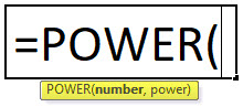
POWER(number, power)

The POWER function syntax has the following arguments:

Number Required. The base number. It can be any real number.
Power Required. The exponent to which the base number is raised.

Remark

The «^» operator can be used instead of POWER to indicate to what power the base number is to be raised, such as in 5^2.

Example

Copy the example data in the following table, and paste it in cell A1 of a new Excel worksheet. For formulas to show results, select them, press F2, and then press Enter. If you need to, you can adjust the column widths to see all the data.

Formula	Description	R esult
=POWER(5,2)	5 squared.	25
=POWER(98.6,3.2)	98.6 raised to the power of 3.2.	2401077.222
=POWER(4,5/4)	4 raised to the power of 5/4.	5.656854249

Need more help?

Источник

In mathematics, we had exponents, the power to a given base number. In Excel, we have a similar built-in function known as the POWER function, which is used to calculate the power of a given number or base. To use this function, we can use the keyword =POWER( in a cell and provide two arguments, one as the number and another as power.

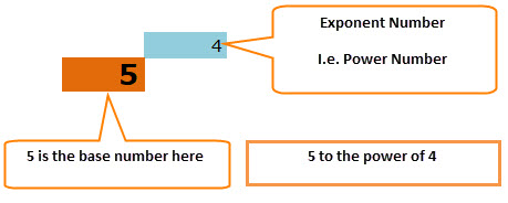
For example, suppose the base number 4 is raised to the power number 3. i.e., 4 cube. =4*4*4 = 64.

A POWER in Excel is a Math/Trigonometric function that computes and returns the result of a number raised to a power. The POWER Excel function takes two arguments: the base (any real number) and the exponent (power that signifies how many times the given number will be multiplied by itself). For example, 5 multiplied by a power of 2 is the same as 5 x5.

Power in Excel
- Formula of POWER Function
- Explanation of POWER Function in Excel
- How to Use POWER Function in Excel
- POWER in Excel Example #1
- POWER in Excel Example #2
- POWER in Excel Example #3
- POWER in Excel Example #4
- Recommended Articles

The Formula of POWER Function

Explanation of POWER Function in Excel

The POWER function in Excel takes both arguments as a numeric value. Hence, the arguments passed are of integer type where the number is the base number, and the POWER is the exponent. Both arguments are required and are not optional.

We can use the POWER function in Excel in many ways, like for mathematical operations. For example, we can use the POWER function equation to compute the relational algebraic functions.

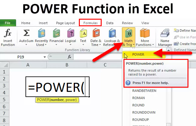
How to Use POWER Function in Excel

The Excel POWER function is very simple and easy to use. Let us understand the working of POWER in Excel by some examples.

You can download this POWER Function Excel Template here – POWER Function Excel Template

POWER in Excel Example #1

We have a POWER function equation y=x^n (x to the power n), where y is dependent on the value of x, and n is the exponent. We also want to draw the graph of this f(x, y) function for given values of x and n=2. For example, the values of x are:

Power

So, in this case, since the value of y depends upon the nth power of x, we will calculate the value of Y using the POWER function in Excel.

1^st value of y will be 2^2 (=POWER(2,2)
2^nd value of y will be 4^2 (=POWER(4,2)
……………………………………………………………
……………………………………………………………
10^th value of y will be 10^2 (=POWER(10,2)

Now, selecting the values of x and y from range B4:K5, choose the graph (in this example, we have chosen the scatter graph with smooth lines) from the “Insert” tab.

So, we get a linear, exponential graph for the given POWER function equation.

POWER in Excel Example #2

In algebra, we have the quadratic POWER function equation, represented as ax2+bx+c=0, where x is unknown, and a, b and c are the coefficients. The solution of this POWER function equation gives the roots of the equation, which are the values of x.

The roots of the quadratic POWER function equation are computed by following mathematical formula:

x = (-b+ (b²-4ac)^1/2)/2a
x = (-b- (b²-4ac)^1/2)/2a

b2-4ac is called discriminant and describes a quadratic POWER function equation’s number of roots.

Now, we have a list of quadratic POWER function equations given in column A. But, first, we need to find the roots of the equations.

^ is the exponential operator used to represent the power (exponent). For example, X2 is the same as x^2.

We have five quadratic POWER function equations, and we will solve them using the formula with the help of the POWER function in Excel to find the roots.

In the first POWER function equation, a=4, b=56, and c = -96. If we mathematically solve them using the above formula, we have the roots -15.5 and 1.5.

To implement this in Excel formula, we will use the POWER function in Excel and the formula will be:

=((-56+POWER(POWER(56,2)-(4*4*(-93)),1/2)))/(2*4) will give the first root and
=((-56-POWER(POWER(56,2)-(4*4*(-93)),1/2)))/(2*4) will give the second root of the equation

So, the complete formula will be,

=”Roots of equations are”&” “&((-56+POWER(POWER(56,2)-(4*4*(-93)),1/2)))/(2*4)&” , “&((-56-POWER(POWER(56,2)-(4*4*(-93)),1/2)))/(2*4)

The formulas are concatenated with the string “Roots of equation are.”

Using the same formula for other POWER function equations, we have:

Output:

POWER in Excel Example #3

So, we can use the POWER function in Excel for different mathematical calculations.

Suppose we have to find out the compound interestCompound interest is the interest charged on the sum of the principal amount and the total interest amassed on it so far. It plays a crucial role in generating higher rewards from an investment.read more for which the formula is:

Amount = Principal (1 + r/n)^nt

Where r is the interest rate, n is the number of times interest is compounded per year, and t is the time.
If an amount of $4,000 is deposited into an account (saving) at an interest rate of 5% annually, compounded monthly, the value of the investment after 5 years can be calculated using the above compound interest formula.
When, Principal = $4000, rate = 5/100 that is 0.05, n =12 (compounded monthly), time =5 years.

We have the formula using the compound interest formula and implementing it into the Excel formula using the POWER function.

=B2*(POWER((1+(B3/B5)),(B4*B5)))

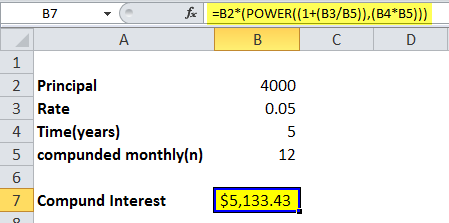
So, the investment balance after 5 years is $5.133.43.

POWER in Excel Example #4

According to Newton’s gravitation law, two bodies at a distance of r from their center of gravity attract each other in the universe according to a gravitational POWER Excel formula.

F = (G*M*m)/r²

When F is the magnitude of the gravitational force, G is called the gravitational constant, M is the mass of the first body, m is the mass of the second body, and r is the distance between the bodies from their center of gravity.

Let us calculate the magnitude of gravitational force by which the sun pulls the earth.

The mass of the sun is 1.98*10^30 kg.
The mass of the earth is 5.97*10^24 kg.
The distance between the sun and the earth is 1.496 x 10^11 meters.
Gravitational constant value is 6.67*10^-11 m3kg-1s-2.

In Excel, if we want to calculate the gravitational force, we will again be using the POWER in Excel that can operate over big numeric values.

So, we can convert the scientific notation values into the POWER Excel formula using the POWER in Excel.
1.98*10^30 will be represented as 1.98*Power(10,30), similarly to other values.
So, the POWER Excel formula to calculate the force will be: = (6.67*POWER(10,-11)*1.98*POWER(10,30)*5.97*POWER(10,24))/POWER(1.496*POWER(10,11),2)

Since the value obtained as force is a big number Excel expressed it scientific notationIn Excel, scientific notation is a specific style of writing numbers in scientific and exponential forms. Scientific notation compactly helps display values, allowing us to compare and use the same in calculations.read more. To change it into a fraction, change the format to the fraction.

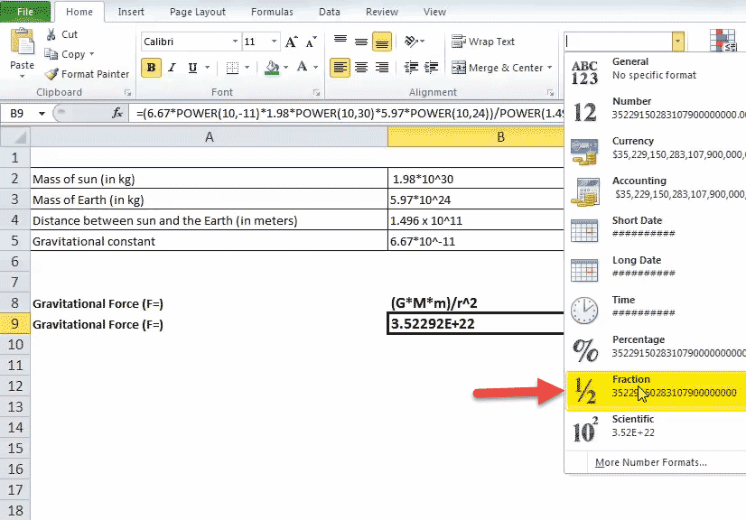
Output:

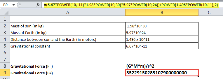
So, the sun pulls the earth with a force of magnitude 35229150283107900000000 Newton.

Summary

The Excel POWER function returns a number raised to a given power. The POWER function is an alternative to the exponent operator (^).

Purpose

Raise a number to a power

Return value

Arguments

number — Number to raise to a power.
power — Power to raise number to (the exponent).

Syntax

Usage notes

The POWER function returns a number raised to a given power. POWER is an alternative to the exponent operator (^) in a math equation.

The POWER function takes two arguments: number and power. Number should be a numeric value, provided as a hardcoded constant or as a cell reference. The power argument functions as the exponent, indicating the power to which number should be raised.

Examples

To raise 2 to the 3rd power, you can use POWER like this:

=POWER(2,3) // returns 8

To raise 2 to the 8th power:

=POWER(2,8) // returns 256

To cube the value in cell A1:

=POWER(A1,3) // cube A1

Fractional exponents

To use the power function with a fractional exponent, enter the fraction directly as the power argument:

=POWER(27,1/3) // returns 3
=POWER(81,1/4) // returns 3
=POWER(256,1/8) // returns 2

Exponent operator

In Excel, exponentiation can also be handled with the exponent (^) operator, so:

=2^2=POWER(2,2)=4
=2^3=POWER(2,3)=8
=2^4=POWER(2,4)=16

Author

Dave Bruns

Hi — I’m Dave Bruns, and I run Exceljet with my wife, Lisa. Our goal is to help you work faster in Excel. We create short videos, and clear examples of formulas, functions, pivot tables, conditional formatting, and charts.

This is the best learning resource I have stumbled upon in many years during the process of my Excel learning.

Get Training

Quick, clean, and to the point training

Learn Excel with high quality video training. Our videos are quick, clean, and to the point, so you can learn Excel in less time, and easily review key topics when needed. Each video comes with its own practice worksheet.

View Paid Training & Bundles

Help us improve Exceljet

Источник

POWER in Excel (Table of Contents)

POWER in Excel
POWER Formula in Excel
How to Use POWER Function in Excel?

POWER in Excel

I still remember the days when my maths teacher beat me almost every day for not remembering the SQUARE ROOT of numbers. I literally cried when maths period is on the way. There are many instances where I bunked the math class just to get away from those beatings from my maths teacher.

Ok, now I need not to remember all those SQUARE ROOTS; instead, I can rely on a beautiful function called the POWER Function.

POWER function helps in raising the number to another number of times to the power.

For example: What is the value of 5 to the square of 3? The answer is 5*5*5 = 125.

POWER Formula in Excel

Below is the POWER Formula:

The Power Function includes two parameters, and both are required arguments.

Number: The number you need to raise the power, i.e. the base number of any real number.
Power: The number of times you need to raise the base number. It is the exponent to raise the base number.

The symbol or operator ^ (caret operator) acts as an exponent. For example: 6^2 = 36. This is not 6 is multiplied by 2 rather 6 * 6 = 36. Six is multiplied by the six itself twice.

The simple equation is 5 * 5 * 5 * 5 = 625

How to Use the POWER Function in Excel?

This POWER function is very simple easy to use. Let us now see how to use the POWER Function with the help of some examples.

You can download this POWER Function in Excel Template here – POWER Function in Excel Template

Example #1

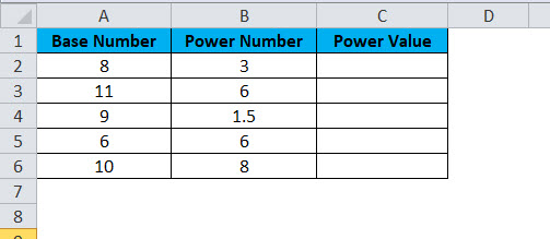
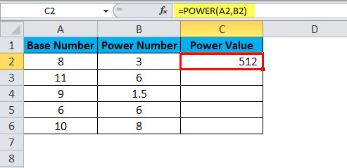
Assume you have base numbers from A2:A6 and the power number (exponential numbers) from B2:B6. Show the power of values in column A by using power numbers in column B.

Apply Power formula in the cell C2

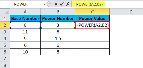
The answer will be:

Drag and drop the formula to other cells.

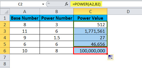
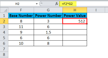
The first value is base number 8 is raised to the power number 3. i.e. 8 cube. =8*8*8 = 512.

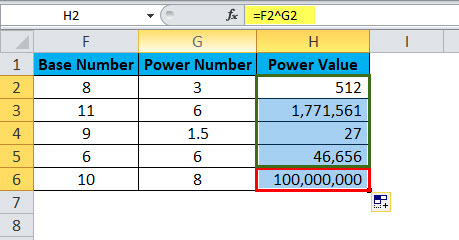
Secondly, base number 11 is raised to the power number 6, i.e. 11 is multiplied 6 times to the 11 itself. =11 * 11* 11* 11* 11* 11 = 17, 71,561. Similarly, all the values have resulted in that way.

Example #2

Use the same data from the above example. Instead of using the POWER Function, we use the caret operator (^) to do the calculation. The results will be the same, though.

Apply formula in the cell H2

The answer will be:

Drag and drop the formula to other cells.

Example #3

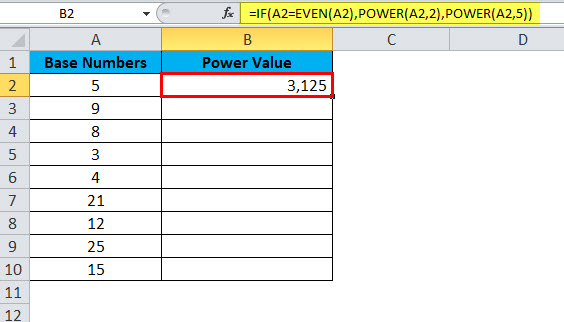
Using POWER Function along with other functions. From the below data, raise all the even numbers power by 2; if the number is not even, then raise the power by 5.

Here, first, we need to test whether the number is even or not. If the number found, raise the power by 2; if not, raise the power by 5.

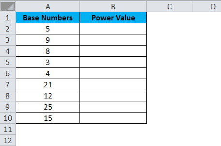
This type of problem can be addressed by using the IF condition to test whether the number is even or not.

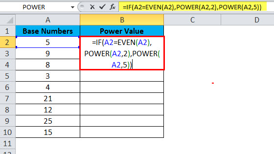
Apply formula in cell B2.

The answer will be:

Drag and drop the formula to other cells.

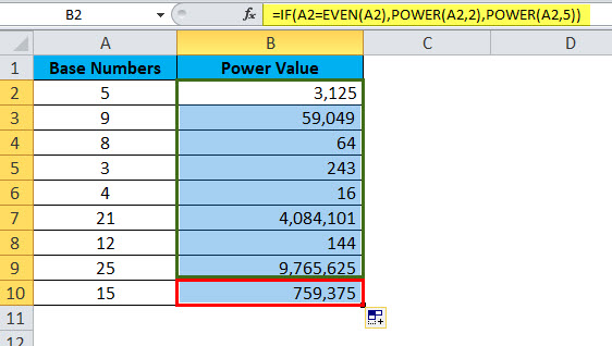
IF condition tests whether the supplied number is equal to an even number or not. =IF(A2=EVEN(A2),
If the IF logic is true then the POWER function will raise the power by 2. =POWER(A2,2),
If the IF logic is false, then the POWER function will raise the power by 5. =POWER(A2,5),

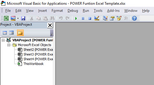
POWER Function in VBA

In VBA, also we can use the POWER function. However, the thing is, we do not get to see many of these live examples in our day-to-day life.

Step 1: Open your VBA editor (ALT + F11).

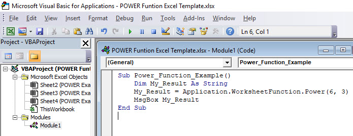
Step 2: Go to insert and insert Module. This would instantly create a new module to write our code for the POWER function.

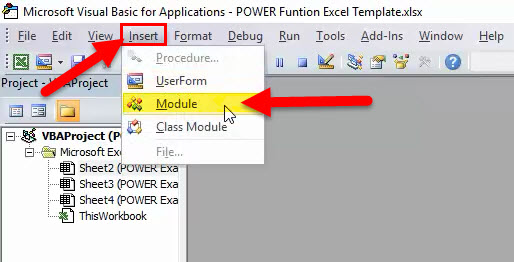
Step 3: Copy and paste the below code inside the new module.

Sub Power_Function_Example () Dim My_Result As String My_Result = Application.WorksheetFunction.Power(6, 3) MsgBox My_Result End Sub

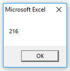
Now your window should look like the one below one.

If you run the code, you will get the below result.

Things to Remember about POWER Function

For a better understanding, we can represent the power function in this way. POWER(X, Y) or POWER(X^Y) both are the same only.
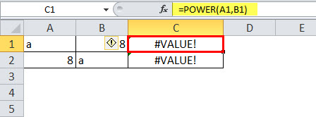
The POWER function is applied only for numerical values. Anything other than numerical values, it will throw the error as #VALUE! If any one of the parameters contains non-numerical values, we will get the error. The below image shows an example of the error.

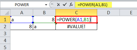
It will show an error.

Description

The Microsoft Excel POWER function returns the result of a number raised to a given power.

The POWER function is a built-in function in Excel that is categorized as a Math/Trig Function. It can be used as a worksheet function (WS) in Excel. As a worksheet function, the POWER function can be entered as part of a formula in a cell of a worksheet.

Syntax

The syntax for the POWER function in Microsoft Excel is:

POWER( number, power )

Parameters or Arguments

number: It is the base number.
power: It is the exponent used to raise the base number to.

Returns

The POWER function returns a numeric value.

Applies To

Excel for Office 365, Excel 2019, Excel 2016, Excel 2013, Excel 2011 for Mac, Excel 2010, Excel 2007, Excel 2003, Excel XP, Excel 2000

Type of Function

Worksheet function (WS)

Example (as Worksheet Function)

Let’s look at some Excel POWER function examples and explore how to use the POWER function as a worksheet function in Microsoft Excel:

Based on the Excel spreadsheet above, the following POWER examples would return:

=POWER(A1, A2)
Result: 81

=POWER(A1, A3)
Result: 140.2961154

=POWER(A2, 2)
Result: 16

Источник

Date yes Add (Subtract) Days to a Date Concatenate Dates Convert Date to Number Convert Date to Text Month Name to Number Create Date Range from Dates Day Number of Year Month Name from Date First Day of Month Add (Subtract) Weeks to a Date If Functions with Dates Max Date Number of Days Between Dates Number of Days in a Month Number of Weeks Between Dates Number of Years Between Dates Split Date & Time into Separate Cells Countdown Remaining Days Insert Dates Random Date Generator Using Dynamic Ranges — Year to Date Values Add (Subtract) Years to a Date Date Formula Examples Extract Day from Date Get Day Name from Date Count Days Left in Month / Year Count Workdays Left in Month / Year Get Last Day of Month Last Business Day of Month / Year Number of Work / Business Days in Month Weekday Abbreviations Auto Populate Dates Number of Months Between Dates Quarter from a Date Years of Service Change Date Format Compare Dates Time yes Add (Subtract) Hours to Time Add (Subtract) Minutes to Time Add (Subtract) Seconds to Time Add Up time (Total Time) Time Differences Change Time Format Convert Minutes to Hours Convert Time to Decimal Convert Time to Hours Convert Time to Minutes Convert Time to Seconds Military Time Round Time to Nearest 15 Minutes Overtime Calculator Number of Hours Between Times Convert Seconds to Minutes, Hours, or Time Count Hours Worked Time Differences Time Format — Show Minutes Seconds Text yes Add Commas to Cells Get First Word from Text Capitalize First Letter Clean & Format Phone #s Remove Extra Trailing / Leading Spaces Add Spaces to Cell Assign Number Value to Text Combine Cells with Comma Combine First and Last Names Convert Text String to Date Convert Text to Number Extract Text From Cell Get Last Word Remove Unwated Characters Extract Text Before or After Character How to Split Text String by Space, Comma, & More Remove Special Characters Remove First Characters from Left Substitute Multiple Values Switch First & Last Names w/ Commas Remove Specific Text from a Cell Extract Text Between Characters (Ex. Parenthesis) Add Leading Zeros to a Number Remove Line Breaks from Text Remove all Numbers from Text Reverse Text Remove Non-Numeric Characters Remove Last Character(s) From Right Separate First and Last Names Separate Text & Numbers Round yes Round Formulas Round Price to Nearest Dollar or Cent Round to Nearest 10, 100, or 1000 Round to Nearest 5 or .5 Round Percentages Round to Significant Figures Count yes Count Blank and Non-blank Cells Count Cells Between Two Numbers Count Cells not Equal to Count if Cells are in Range Count Times Word Appears in Cell Count Words in Cell Count Specific Characters in Column Count Total Number of Characters in Column Count Cells that Equal one of two Results Count Cells that do not Contain Count Cells that Contain Specific Text Count Unique Values in Range Countif — Multiple Criteria Count Total Number of Cells in Range Count Cells with Any Text Count Total Cells in a Table Lookup yes Two Dimensional VLOOKUP VLOOKUP Simple Example Vlookup — Multiple Matches Case Sensitive Lookup Case Sensitive VLOOKUP Sum if — VLOOKUP Case Sensitive Lookup Case Sensitive VLOOKUP Find Duplicates w/ VLOOKUP or MATCH INDEX MATCH MATCH Lookup — Return Cell Address (Not Value) Lookup Last Value in Column or Row Reverse VLOOKUP (Right to Left) Risk Score Bucket with VLOOKUP Sum with a VLOOKUP Function VLOOKUP & INDIRECT VLOOKUP Concatenate VLOOKUP Contains (Partial Match) 17 Reasons Why Your XLOOKUP is Not Working Double (Nested) XLOOKUP — Dynamic Columns IFERROR (& IFNA) XLOOKUP Lookup Min / Max Value Nested VLOOKUP Top 11 Alternatives to VLOOKUP (Updated 2022!) VLOOKUP – Dynamic Column Reference VLOOKUP – Fix #N/A Error VLOOKUP – Multiple Sheets at Once VLOOKUP & HLOOKUP Combined VLOOKUP & MATCH Combined VLOOKUP Between Worksheets or Spreadsheets VLOOKUP Duplicate Values VLOOKUP Letter Grades VLOOKUP Return Multiple Columns VLOOKUP Returns 0? Return Blank Instead VLOOKUP w/o #N/A Error XLOOKUP Multiple Sheets at Once XLOOKUP Between Worksheets or Spreadsheets XLOOKUP by Date XLOOKUP Duplicate Values XLOOKUP Multiple Criteria XLOOKUP Return Multiple Columns XLOOKUP Returns 0? Return Blank Instead XLOOKUP Text XLOOKUP with IF XLOOKUP With If Statement Misc. yes Sort Multiple Columns Use Cell Value in Formula Percentage Change Between Numbers Percentage Breakdown Rank Values Add Spaces to Cell CAGR Formula Average Time Decimal Part of Number Integer Part of a Number Compare Items in a List Dealing with NA() Errors Get Worksheet Name Wildcard Characters Hyperlink to Current Folder Compound Interest Formula Percentage Increase Create Random Groups Sort with the Small and Large Functions Non-volatile Function Alternatives Decrease a Number by a Percentage Calculate Percent Variance Profit Margin Calculator Convert Column Number to Letter Get Full Address of Named Range Insert File Name Insert Path Latitute / Longitude Functions Replace Negative Values Reverse List Range Convert State Name to Abbreviation Create Dynamic Hyperlinks Custom Sort List with Formula Data Validation — Custom Formulas Dynamic Sheet Reference (INDIRECT) Reference Cell in Another Sheet or Workbook Get Cell Value by Address Get Worksheet Name Increment Cell Reference List Sheet Names List Skipped Numbers in Sequence Return Address of Max Value in Range Search by Keywords Select Every Other (or Every nth) Row Basics yes Cell Reference Basics — A1, R1C1, 3d, etc. Add Up (Sum) Entire Column or Row Into to Dynamic Array Formulas Conversions yes Convert Time Zones Convert Celsius to Fahrenheit Convert Pounds to Kilograms Convert Time to Unix Time Convert Feet to Meters Convert Centimeters to Inches Convert Kilometers to Miles Convert Inches to Feet Convert Date to Julian Format Convert Column Letter to Number Tests yes Test if a Range Contains any Text Test if any Cell in Range is Number Test if a Cell Contains a Specific Value Test if Cell Contains Any Number Test if Cell Contains Specific Number Test if Cell is Number or Text If yes Percentile If Subtotal If Sumproduct If Large If and Small If Median If Concatentate If Max If Rank If TEXTJOIN If Sum yes Sum if — Begins With / Ends With Sum if — Month or Year to Date Sum if — By Year Sum if — Blank / Non-Blank Sum if — Horizontal Sum Count / Sum If — Cell Color INDIRECT Sum Sum If — Across Multiple Sheets Sum If — By Month Sum If — Cells Not Equal To Sum If — Not Blank Sum if — Between Values Sum If — Week Number Sum Text Sum if — By Category or Group Sum if — Cell Contains Specific Text (Wildcards) Sum if — Date Rnage Sum if — Dates Equal Sum if — Day of Week Sum if — Greater Than Sum if — Less Than Average yes Average Non-Zero Values Average If — Not Blank Average — Ignore 0 Average — Ignore Errors Math yes Multiplication Table Cube Roots nth Roots Square Numbers Square Roots Calculations yes Calculate a Ratio Calculate Age KILLLLLLL Calculate Loan Payments GPA Formula Calculate VAT Tax How to Grade Formulas Find yes Find a Number in a Column / Workbook Find Most Frequent Numbers Find Smallest n Values Find nth Occurance of Character in Text Find and Extract Number from String Find Earliest or Latest Date Based on Criteria Find First Cell with Any Value Find Last Row Find Last Row with Data Find Missing Values Find Largest n Values Most Frequent Number Conditional Formatting yes Conditional Format — Dates & Times Conditional Format — Highlight Blank Cells New Functions XLOOKUP Replaces VLOOKUP, HLOOKUP, and INDEX / MATCH Logical yes AND Checks whether all conditions are met. TRUE/FALSE IF If condition is met, do something, if not, do something else. IFERROR If result is an error then do something else. NOT Changes TRUE to FALSE and FALSE to TRUE. OR Checks whether any conditions are met. TRUE/FALSE XOR Checks whether one and only one condition is met. TRUE/FALSE Lookup & Reference yes FALSE The logical value: FALSE. TRUE The logical value: TRUE. ADDRESS Returns a cell address as text. AREAS Returns the number of areas in a reference. CHOOSE Chooses a value from a list based on it’s position number. COLUMN Returns the column number of a cell reference. COLUMNS Returns the number of columns in an array. HLOOKUP Lookup a value in the first row and return a value. HYPERLINK Creates a clickable link. INDEX Returns a value based on it’s column and row numbers. INDIRECT Creates a cell reference from text. LOOKUP Looks up values either horizontally or vertically. MATCH Searches for a value in a list and returns its position. OFFSET Creates a reference offset from a starting point. ROW Returns the row number of a cell reference. ROWS Returns the number of rows in an array. TRANSPOSE Flips the oriention of a range of cells. VLOOKUP Lookup a value in the first column and return a value. Date & Time yes DATE Returns a date from year, month, and day. DATEDIF Number of days, months or years between two dates. DATEVALUE Converts a date stored as text into a valid date DAY Returns the day as a number (1-31). DAYS Returns the number of days between two dates. DAYS360 Returns days between 2 dates in a 360 day year. EDATE Returns a date, n months away from a start date. EOMONTH Returns the last day of the month, n months away date. HOUR Returns the hour as a number (0-23). MINUTE Returns the minute as a number (0-59). MONTH Returns the month as a number (1-12). NETWORKDAYS Number of working days between 2 dates. NETWORKDAYS.INTL Working days between 2 dates, custom weekends. NOW Returns the current date and time. SECOND Returns the second as a number (0-59) TIME Returns the time from a hour, minute, and second. TIMEVALUE Converts a time stored as text into a valid time. TODAY Returns the current date. WEEKDAY Returns the day of the week as a number (1-7). WEEKNUM Returns the week number in a year (1-52). WORKDAY The date n working days from a date. WORKDAY.INTL The date n working days from a date, custom weekends. YEAR Returns the year. YEARFRAC Returns the fraction of a year between 2 dates. Engineering yes CONVERT Convert number from one unit to another. Financial yes FV Calculates the future value. PV Calculates the present value. NPER Calculates the total number of payment periods. PMT Calculates the payment amount. RATE Calculates the interest Rate. NPV Calculates the net present value. IRR The internal rate of return for a set of periodic CFs. XIRR The internal rate of return for a set of non-periodic CFs. PRICE Calculates the price of a bond. YIELD Calculates the bond yield. INTRATE The interest rate of a fully invested security. Information yes CELL Returns information about a cell. ERROR.TYPE Returns a value representing the cell error. ISBLANK Test if cell is blank. TRUE/FALSE ISERR Test if cell value is an error, ignores #N/A. TRUE/FALSE ISERROR Test if cell value is an error. TRUE/FALSE ISEVEN Test if cell value is even. TRUE/FALSE ISFORMULA Test if cell is a formula. TRUE/FALSE ISLOGICAL Test if cell is logical (TRUE or FALSE). TRUE/FALSE ISNA Test if cell value is #N/A. TRUE/FALSE ISNONTEXT Test if cell is not text (blank cells are not text). TRUE/FALSE ISNUMBER Test if cell is a number. TRUE/FALSE ISODD Test if cell value is odd. TRUE/FALSE ISREF Test if cell value is a reference. TRUE/FALSE ISTEXT Test if cell is text. TRUE/FALSE N Converts a value to a number. NA Returns the error: #N/A. TYPE Returns the type of value in a cell. Math yes ABS Calculates the absolute value of a number. AGGREGATE Define and perform calculations for a database or a list. CEILING Rounds a number up, to the nearest specified multiple. COS Returns the cosine of an angle. DEGREES Converts radians to degrees. DSUM Sums database records that meet certain criteria. EVEN Rounds to the nearest even integer. EXP Calculates the exponential value for a given number. FACT Returns the factorial. FLOOR Rounds a number down, to the nearest specified multiple. GCD Returns the greatest common divisor. INT Rounds a number down to the nearest integer. LCM Returns the least common multiple. LN Returns the natural logarithm of a number. LOG Returns the logarithm of a number to a specified base. LOG10 Returns the base-10 logarithm of a number. MOD Returns the remainder after dividing. MROUND Rounds a number to a specified multiple. ODD Rounds to the nearest odd integer. PI The value of PI. POWER Calculates a number raised to a power. PRODUCT Multiplies an array of numbers. QUOTIENT Returns the integer result of division. RADIANS Converts an angle into radians. RAND Calculates a random number between 0 and 1. RANDBETWEEN Calculates a random number between two numbers. ROUND Rounds a number to a specified number of digits. ROUNDDOWN Rounds a number down (towards zero). ROUNDUP Rounds a number up (away from zero). SIGN Returns the sign of a number. SIN Returns the sine of an angle. SQRT Calculates the square root of a number. SUBTOTAL Returns a summary statistic for a series of data. SUM Adds numbers together. SUMIF Sums numbers that meet a criteria. SUMIFS Sums numbers that meet multiple criteria. SUMPRODUCT Multiplies arrays of numbers and sums the resultant array. TAN Returns the tangent of an angle. TRUNC Truncates a number to a specific number of digits. Stats yes AVERAGE Averages numbers. AVERAGEA Averages numbers. Includes text & FALSE =0, TRUE =1. AVERAGEIF Averages numbers that meet a criteria. AVERAGEIFS Averages numbers that meet multiple criteria. CORREL Calculates the correlation of two series. COUNT Counts cells that contain a number. COUNTA Count cells that are non-blank. COUNTBLANK Counts cells that are blank. COUNTIF Counts cells that meet a criteria. COUNTIFS Counts cells that meet multiple criteria. FORECAST Predict future y-values from linear trend line. FREQUENCY Counts values that fall within specified ranges. GROWTH Calculates Y values based on exponential growth. INTERCEPT Calculates the Y intercept for a best-fit line. LARGE Returns the kth largest value. LINEST Returns statistics about a trendline. MAX Returns the largest number. MEDIAN Returns the median number. MIN Returns the smallest number. MODE Returns the most common number. PERCENTILE Returns the kth percentile. PERCENTILE.INC Returns the kth percentile. Where k is inclusive. PERCENTILE.EXC Returns the kth percentile. Where k is exclusive. QUARTILE Returns the specified quartile value. QUARTILE.INC Returns the specified quartile value. Inclusive. QUARTILE.EXC Returns the specified quartile value. Exclusive. RANK Rank of a number within a series. RANK.AVG Rank of a number within a series. Averages. RANK.EQ Rank of a number within a series. Top Rank. SLOPE Calculates the slope from linear regression. SMALL Returns the kth smallest value. STDEV Calculates the standard deviation. STDEV.P Calculates the SD of an entire population. STDEV.S Calculates the SD of a sample. STDEVP Calculates the SD of an entire population TREND Calculates Y values based on a trendline. Text yes CHAR Returns a character specified by a code. CLEAN Removes all non-printable characters. CODE Returns the numeric code for a character. CONCATENATE Combines text together. DOLLAR Converts a number to text in currency format. EXACT Test if cells are exactly equal. Case-sensitive. TRUE/FALSE FIND Locates position of text within a cell.Case-sensitive. LEFT Truncates text a number of characters from the left. LEN Counts number of characters in text. LOWER Converts text to lower case. MID Extracts text from the middle of a cell. PROPER Converts text to proper case. REPLACE Replaces text based on it’s location. REPT Repeats text a number of times. RIGHT Truncates text a number of characters from the right. SEARCH Locates position of text within a cell.Not Case-sensitive. SUBSTITUTE Finds and replaces text. Case-sensitive. TEXT Converts a value into text with a specific number format. TRIM Removes all extra spaces from text. UPPER Converts text to upper case. VALUE Converts a number stored as text into a number.

Источник

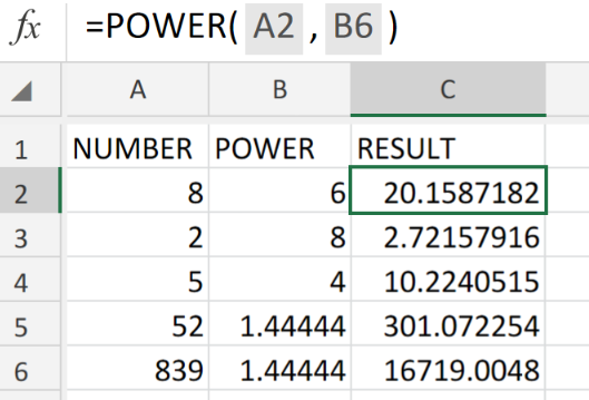Figure 1. of Excel POWER Function.

In the event that we want to determine a very small level of tolerance for vast distances. At some point we will have to raise a number to a specific power. We are going to utilize the Excel POWER Function. This article will walk through how to do it.

Generic Formula

POWER(number, power)

The POWER Function will calculate a number raised to a specific power. The formula syntax has the following components;

number – the number value which we desire to raise to a certain power. This can be any real number.
power – the exponential value to which we are going to raise our base number.

How to use the Excel POWER Function.

We can achieve this by following three simple steps!

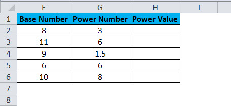
Collect the data available to us for checking, in our Excel sheet. See example illustrated below;

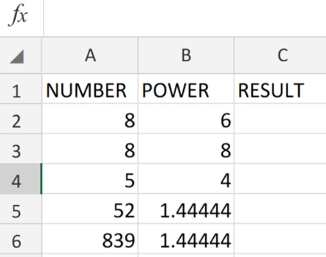Figure 2. of Number Values for the POWER Function in Excel.

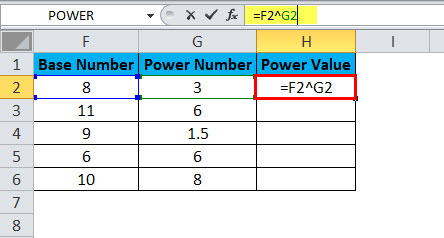
Our purpose here is to exponentially raise the number values in column A to the power Values specified in column B of our worksheet. The formula syntax which we will enter into the formula bar for cell C2, for the desired result is as follows;

=POWER(A2,B6)

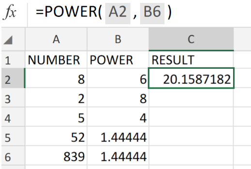Figure 3. of the POWER Function in Excel.

Modify and copy the formula syntax into the other cells in column C of the example illustrated below to achieve the desired results.

Figure 4. of the POWER Function in Excel.

The POWER Function operates like an exponential value in a basic mathematical equation.

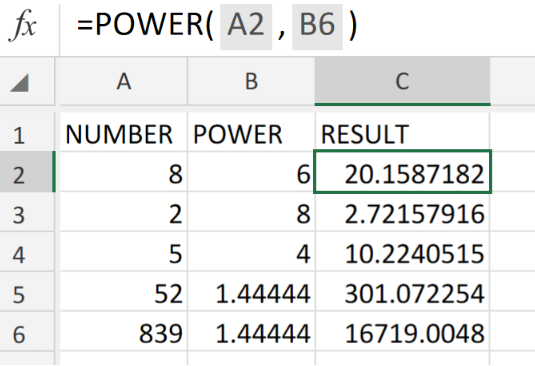Figure 5. of Final Result.

Instant Connection to an Expert through our Excelchat Service

Our live Excelchat Service is here for you. We have Excel Experts available 24/7 to answer any Excel questions you may have. Guaranteed connection within 30 seconds and a customized solution for you within 20 minutes.

Did this post not answer your question? Get a
solution from
connecting
with the expert.

Another blog reader asked this question today on Excelchat:

what is 2 to the 431 power. what is 3 to 421 power

An Excelchat Expert solved this problem in 24 mins!

Источник

A very common question asked by excel users who play with numbers in excel is – “How to perform raised to the power operation in excel?”. There are two answers to this. The first method is by using the caret (^) symbol on your keyboard and the alternative way is by using an excel formula – the POWER function in excel.

In this tutorial, we would learn how to use the Excel POWER function to do raise to operation in excel along with examples.

Table of Contents

What is Use of Raised to the Power Operation?
When To Use Excel Power Formula
Syntax and Arguments
POWER Excel Function – Examples
Alternative Way to Find Exponential Value in Excel

Here we go 😎

What is Use of Raised to the Power Operation?

The raise to the power operation is a mathematical operation wherein you multiply a number with the same number n number of times.

Suppose you want to multiply the number 3 by itself seven times.

One way to denote this is by writing the number ‘3’ for seven times each separated by multiplication sign.

3 X 3 X 3 X 3 X 3 X 3 X 3

Interestingly, there is a more convenient and easy way to write this. Simply place the number 7 on the top right corner of the number 3, like this:

3⁷

The above is pronounced like this – “3 raised to the power 7“.

The another name for this is “exponents”.

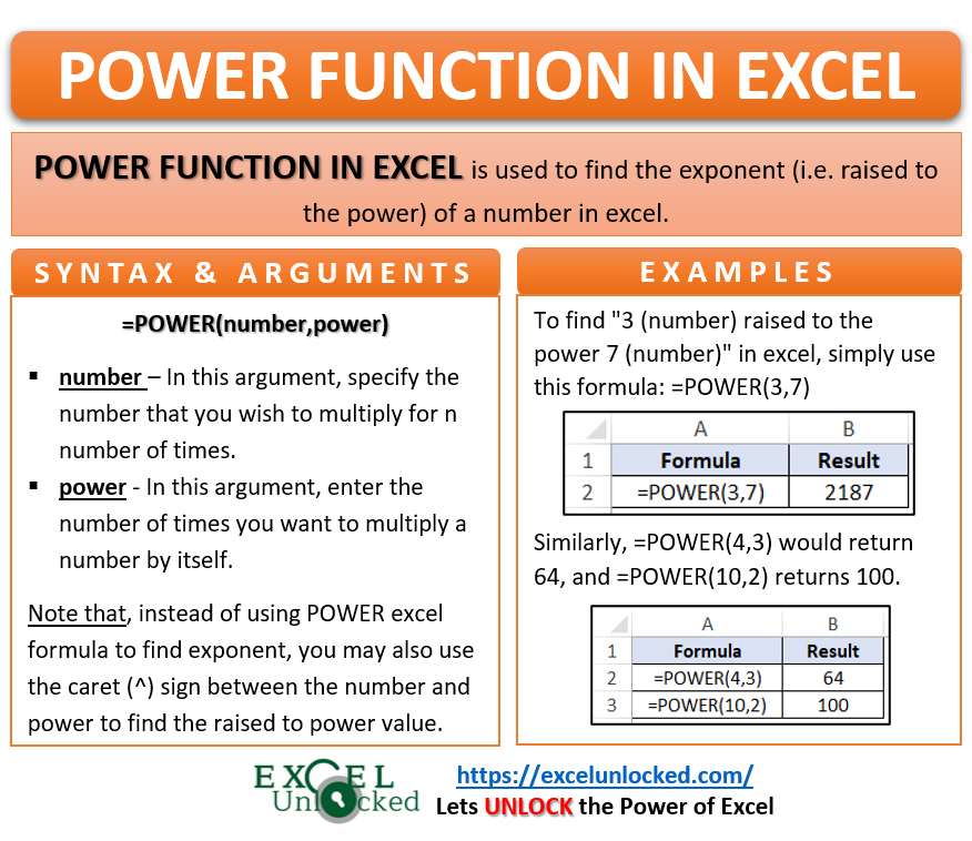
When To Use Excel Power Formula

The Excel POWER Formula is an in-built mathematical function that is used to find the exponent (i.e. raised to the power) of a number in excel. It is a useful function for multiplying a number with the same number multiple times in excel.

As a result, this formula returns a value raised to the power.

Syntax and Arguments

=POWER(number,power)

The two arguments of the POWER formula in excel are explained as below:

number – In this argument, specify the number that you wish to multiply for n number of times.

power – In this argument, enter the exponential value i.e. the number of times you want to multiply the number by itself.

Infographic - POWER Formula Function in Excel

POWER Excel Function – Examples

Let us take the same examples learned in the above section.

To find “3 (number) raised to the power 7 (number)” in excel, simply use the following formula:

=POWER(3,7)

As a result, excel would return the output as 2187.

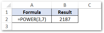
Explanation – In the above examples, the excel POWER formula multiplies the number argument ‘3’ for ‘7’ times (power argument), and returns its result.

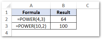
Similarly, =POWER(4,3) would return 64, and =POWER(10,2) returns 100.

Alternative Way to Find Exponential Value in Excel

As learned in the introduction section of this blog, there are two ways to find the exponent in excel. The first one is to use the Excel POWER function and another way is to use caret (^) sign to find raised to the power.

In this section, we would learn how to use the caret (^) symbol to find exponents in excel.

To find the value of 3 raised to the power 7 in excel, simply put the caret sign (^) in between the two numbers (the number and the power), like this:

=3^7

As a result, excel would return the same output – 2187.

Thank You 🙂

Applications of SQRT Function in Excel
CHAR Function in Excel – Return Character By Code
COLUMN Function in Excel – Get Cell Column Number
N Function in Excel – Usage and Examples
Custom Columns in Table in Excel Power Query
How to use Excel Fill Handle Tool

Источник

Description

Syntax

Remark

Example

Need more help?

Table of contents

Explanation of POWER Function in Excel

How to Use POWER Function in Excel

POWER in Excel Example #1

POWER in Excel Example #2

POWER in Excel Example #3

POWER in Excel Example #4

Recommended Articles

Summary

Purpose

Return value

Arguments

Syntax

Usage notes

Examples

Fractional exponents

Exponent operator

Dave Bruns

Get Training

Quick, clean, and to the point training

Help us improve Exceljet

POWER in Excel

POWER Formula in Excel

How to Use the POWER Function in Excel?

Example #1

Example #2

Example #3

POWER Function in VBA

Things to Remember about POWER Function

Recommended Articles

Description

Syntax

Parameters or Arguments

Returns

Applies To

Type of Function

Example (as Worksheet Function)

Generic Formula

How to use the Excel POWER Function.

Instant Connection to an Expert through our Excelchat Service

Did this post not answer your question? Get a solution from connecting with the expert.

What is Use of Raised to the Power Operation?

When To Use Excel Power Formula

Syntax and Arguments

POWER Excel Function – Examples

Alternative Way to Find Exponential Value in Excel

RELATED POSTS

Did this post not answer your question? Get a
solution from
connecting
with the expert.