Построить график в excel python - Word и Excel - помощь в работе с программами

Improve Article

Save Article

Like Article

Read

Discuss

Improve Article

Save Article

Like Article

Prerequisite: Python | Plotting charts in excel sheet using openpyxl module | Set – 1 Openpyxl is a Python library using which one can perform multiple operations on excel files like reading, writing, arithmetic operations and plotting graphs. Charts are composed of at least one series of one or more data points. Series themselves are comprised of references to cell ranges. Let’s see how to plot Scatter, Bubble, Pie, 3D Pie Chart on an excel sheet using openpyxl. For plotting the charts on an excel sheet, firstly, create chart object of specific chart class( i.e ScatterChart, PieChart etc.). After creating chart objects, insert data in it and lastly, add that chart object in the sheet object. Let’s see how to plot different charts using realtime data. Code #1 : Plot the Bubble Chart. Bubble charts are similar to scatter charts but use a third dimension to determine the size of the bubbles. Charts can include multiple series. For plotting the bubble chart on an excel sheet, use BubbleChart class from openpyxl.chart submodule.

Python3

import openpyxl

from openpyxl.chart import BubbleChart, Reference, Series

wb = openpyxl.Workbook()

sheet = wb.active

rows = [

("Number of Products", "Sales in USD", "Market share"),

(14, 12200, 15),

(20, 60000, 33),

(18, 24400, 10),

(22, 32000, 42),

]

for row in rows:

sheet.append(row)

chart = BubbleChart()

xvalues = Reference(sheet, min_col = 1,

min_row = 2, max_row = 5)

yvalues = Reference(sheet, min_col = 2,

min_row = 2, max_row = 5)

size = Reference(sheet, min_col = 3,

min_row = 2, max_row = 5)

series = Series(values = yvalues, xvalues = xvalues,

zvalues = size, title ="2013")

chart.series.append(series)

chart.title = " BUBBLE-CHART "

chart.x_axis.title = " X_AXIS "

chart.y_axis.title = " Y_AXIS "

sheet.add_chart(chart, "E2")

wb.save("bubbleChart.xlsx")

Output: 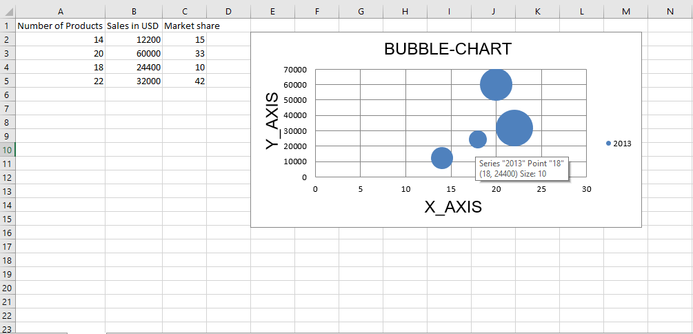Code #2 : Plot the Scatter Chart Scatter, or xy charts are similar to some line charts. For plotting the Scatter chart on an excel sheet, use ScatterChart class from openpyxl.chart submodule.

Python3

import openpyxl

from openpyxl.chart import ScatterChart, Reference, Series

wb = openpyxl.Workbook()

sheet = wb.active

rows = [

("Number of Products", "Sales in USD", "Market share"),

(14, 12200, 15),

(20, 60000, 33),

(18, 24400, 10),

(22, 32000, 42),

]

for row in rows:

sheet.append(row)

chart = ScatterChart()

xvalues = Reference(sheet, min_col = 1,

min_row = 2, max_row = 5)

yvalues = Reference(sheet, min_col = 2,

min_row = 2, max_row = 5)

size = Reference(sheet, min_col = 3,

min_row = 2, max_row = 5)

series = Series(values = yvalues, xvalues = xvalues,

zvalues = size, title ="2013")

chart.series.append(series)

chart.title = " SCATTER-CHART "

chart.x_axis.title = " X_AXIS "

chart.y_axis.title = " Y_AXIS "

sheet.add_chart(chart, "E2")

wb.save(" ScatterChart.xlsx")

Output: 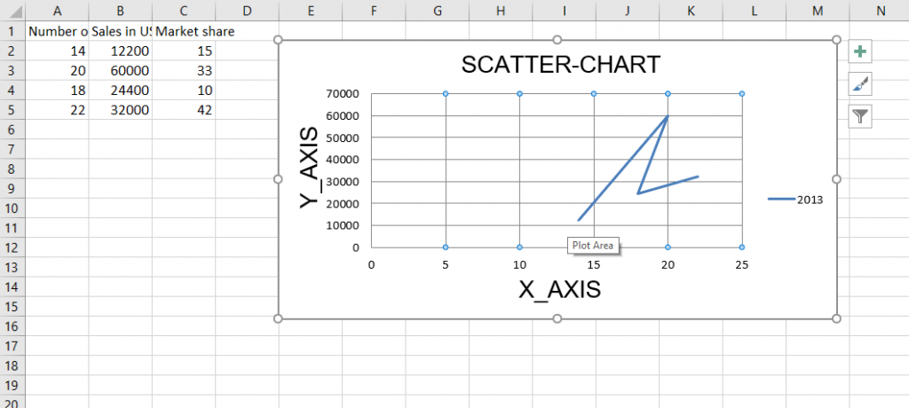Code #3 : Plot the Pie Chart Pie charts plot data as slices of a circle with each slice representing the percentage of the whole. Slices are plotted in a clockwise direction with 0° being at the top of the circle. Pie charts can only take a single series of data. For plotting the Pie chart on an excel sheet, use PieChart class from openpyxl.chart submodule.

Python

import openpyxl

from openpyxl.chart import PieChart, Reference

wb = openpyxl.Workbook()

sheet = wb.active

datas = [

['Pie', 'Sold'],

['Apple', 50],

['Cherry', 30],

['Pumpkin', 10],

['Chocolate', 40],

]

for row in datas:

sheet.append(row)

chart = PieChart()

labels = Reference(sheet, min_col = 1,

min_row = 2, max_row = 5)

data = Reference(sheet, min_col = 2,

min_row = 1, max_row = 5)

chart.add_data(data, titles_from_data = True)

chart.set_categories(labels)

chart.title = " PIE-CHART "

sheet.add_chart(chart, "E2")

wb.save(" PieChart.xlsx")

Output: 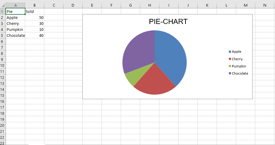Code #4: Plot the Bar Chart For plotting the 3D pie chart on an excel sheet, use PieChart3D class from openpyxl.chart submodule.

Python3

import openpyxl

from openpyxl.chart import PieChart3D, Reference

wb = openpyxl.Workbook()

sheet = wb.active

datas = [

['Pie', 'Sold'],

['Apple', 50],

['Cherry', 30],

['Pumpkin', 10],

['Chocolate', 40],

]

for row in datas:

sheet.append(row)

chart = PieChart3D()

labels = Reference(sheet, min_col = 1,

min_row = 2, max_row = 5)

data = Reference(sheet, min_col = 2,

min_row = 1, max_row = 5)

chart.add_data(data, titles_from_data = True)

chart.set_categories(labels)

chart.title = " 3DPIE-CHART "

sheet.add_chart(chart, "E2")

wb.save(" 3DPieChart.xlsx")

Output: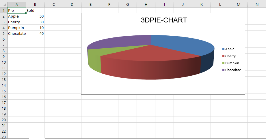

Like Article

Save Article

Vote for difficulty

Current difficulty :
Medium

Источник

This section explains how to work with some of the options and features of
The Chart Class.

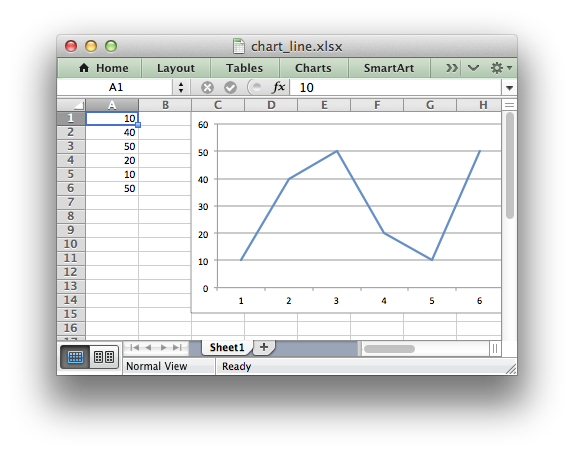
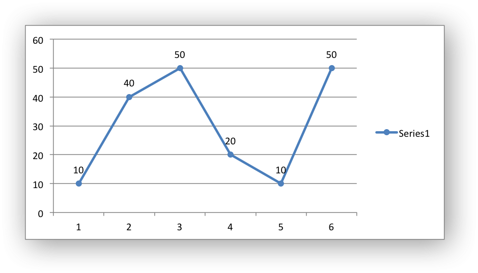
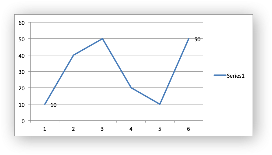
The majority of the examples in this section are based on a variation of the
following program:

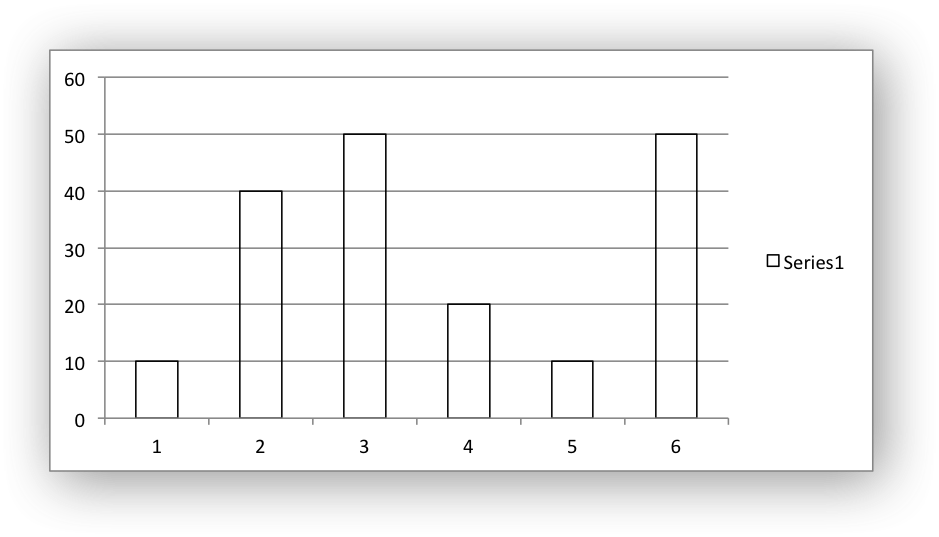
import xlsxwriter

workbook = xlsxwriter.Workbook('chart_line.xlsx')
worksheet = workbook.add_worksheet()

# Add the worksheet data to be plotted.
data = [10, 40, 50, 20, 10, 50]
worksheet.write_column('A1', data)

# Create a new chart object.
chart = workbook.add_chart({'type': 'line'})

# Add a series to the chart.
chart.add_series({'values': '=Sheet1!$A$1:$A$6'})

# Insert the chart into the worksheet.
worksheet.insert_chart('C1', chart)

workbook.close()

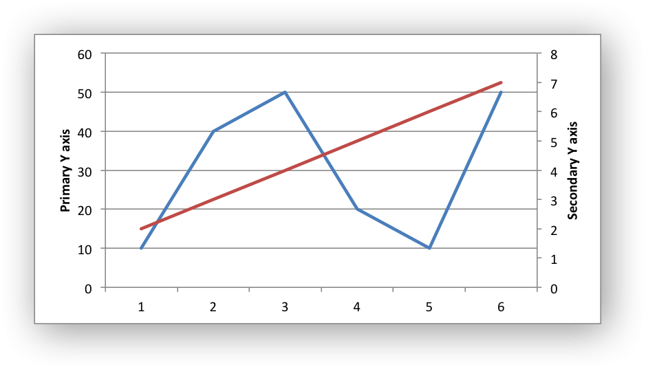
Chart Value and Category Axes

When working with charts it is important to understand how Excel
differentiates between a chart axis that is used for series categories and a
chart axis that is used for series values.

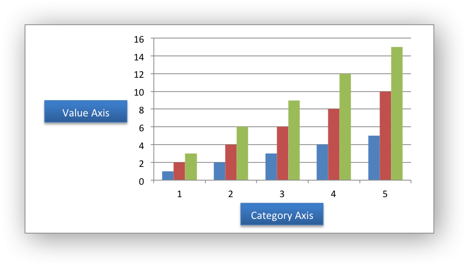
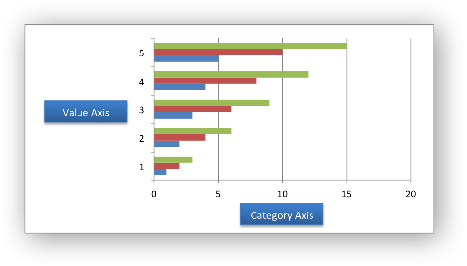
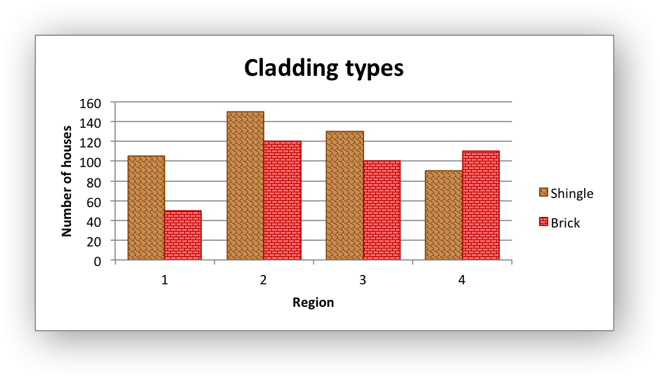
In the majority of Excel charts the X axis is the category axis and each
of the values is evenly spaced and sequential. The Y axis is the value
axis and points are displayed according to their value:

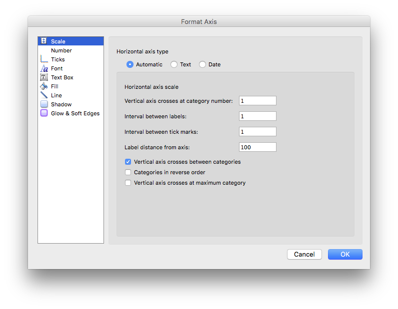
Excel treats these two types of axis differently and exposes different
properties for each. For example, here are the properties for a category axis:

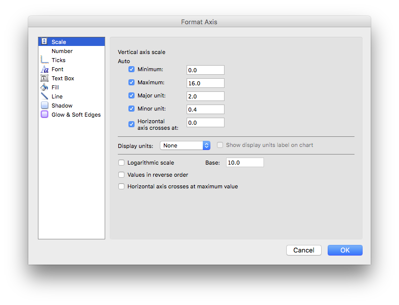
Here are properties for a value axis:

As such, some of the XlsxWriter axis properties can be set for a value
axis, some can be set for a category axis and some properties can be set for
both. For example reverse can be set for either category or value axes while the
min and max properties can only be set for value axes (and Date Axes).
The documentation calls out the type of axis to which properties apply.

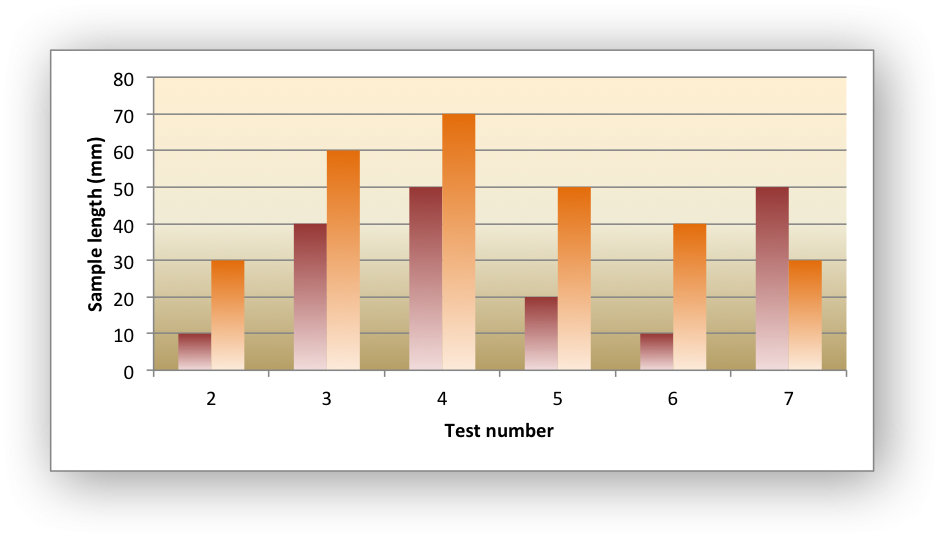
For a Bar chart the Category and Value axes are reversed:

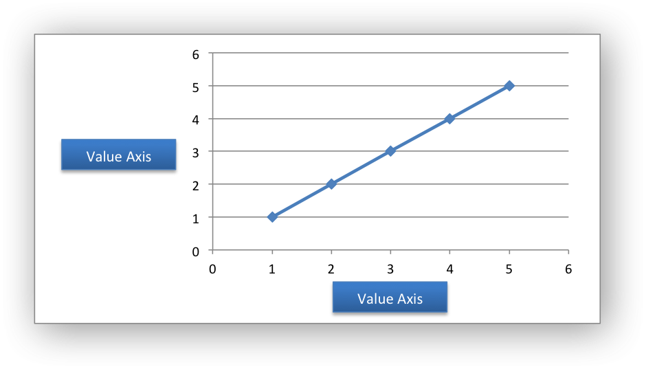
A Scatter chart (but not a Line chart) has 2 value axes:

Date Category Axes are a special type of category axis that give them
some of the properties of values axes such as min and max when used
with date or time values.

Chart Series Options

This following sections detail the more complex options of the
add_series() Chart method:

marker
trendline
y_error_bars
x_error_bars
data_labels
points
smooth

Chart series option: Marker

The marker format specifies the properties of the markers used to distinguish
series on a chart. In general only Line and Scatter chart types and trendlines
use markers.

The following properties can be set for marker formats in a chart:

type
size
border
fill
pattern
gradient

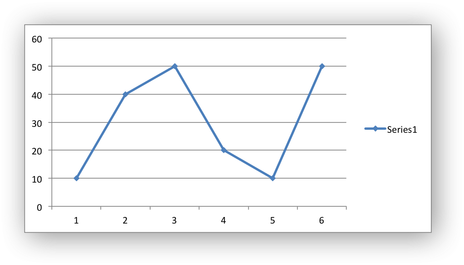
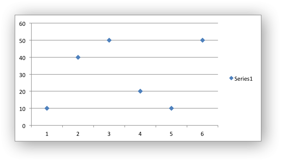
The type property sets the type of marker that is used with a series:

chart.add_series({
    'values': '=Sheet1!$A$1:$A$6',
    'marker': {'type': 'diamond'},
})

The following type properties can be set for marker formats in a chart.
These are shown in the same order as in the Excel format dialog:

automatic
none
square
diamond
triangle
x
star
short_dash
long_dash
circle
plus

The automatic type is a special case which turns on a marker using the
default marker style for the particular series number:

chart.add_series({
    'values': '=Sheet1!$A$1:$A$6',
    'marker': {'type': 'automatic'},
})

If automatic is on then other marker properties such as size, border or
fill cannot be set.

The size property sets the size of the marker and is generally used in
conjunction with type:

chart.add_series({
    'values': '=Sheet1!$A$1:$A$6',
    'marker': {'type': 'diamond', 'size': 7},
})

Nested border and fill properties can also be set for a marker:

chart.add_series({
    'values': '=Sheet1!$A$1:$A$6',
    'marker': {
        'type': 'square',
        'size': 8,
        'border': {'color': 'black'},
        'fill':   {'color': 'red'},
    },
})

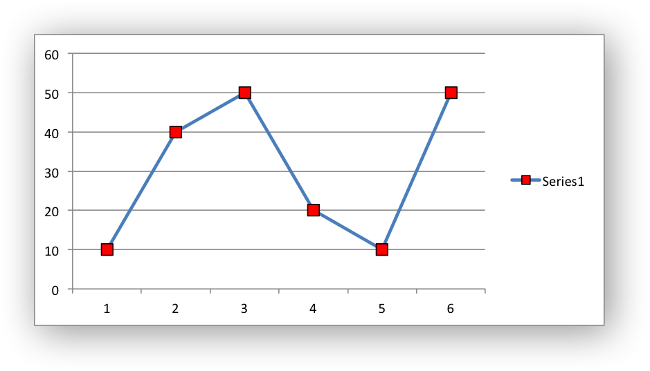
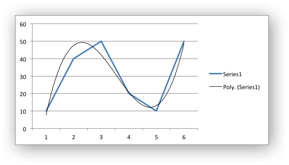
Chart series option: Trendline

A trendline can be added to a chart series to indicate trends in the data such
as a moving average or a polynomial fit.

The following properties can be set for trendlines in a chart series:

type
order               (for polynomial trends)
period              (for moving average)
forward             (for all except moving average)
backward            (for all except moving average)
name
line
intercept           (for exponential, linear and polynomial only)
display_equation    (for all except moving average)
display_r_squared   (for all except moving average)

The type property sets the type of trendline in the series:

chart.add_series({
    'values':    '=Sheet1!$A$1:$A$6',
    'trendline': {'type': 'linear'},
})

The available trendline types are:

exponential
linear
log
moving_average
polynomial
power

A polynomial trendline can also specify the order of the polynomial.
The default value is 2:

chart.add_series({
    'values': '=Sheet1!$A$1:$A$6',
    'trendline': {
        'type': 'polynomial',
        'order': 3,
    },
})

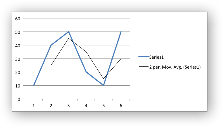
A moving_average trendline can also specify the period of the moving
average. The default value is 2:

chart.add_series({
    'values': '=Sheet1!$A$1:$A$6',
    'trendline': {
        'type': 'moving_average',
        'period': 2,
    },
})

The forward and backward properties set the forecast period of the
trendline:

chart.add_series({
    'values': '=Sheet1!$A$1:$A$6',
    'trendline': {
        'type': 'polynomial',
        'order': 2,
        'forward': 0.5,
        'backward': 0.5,
    },
})

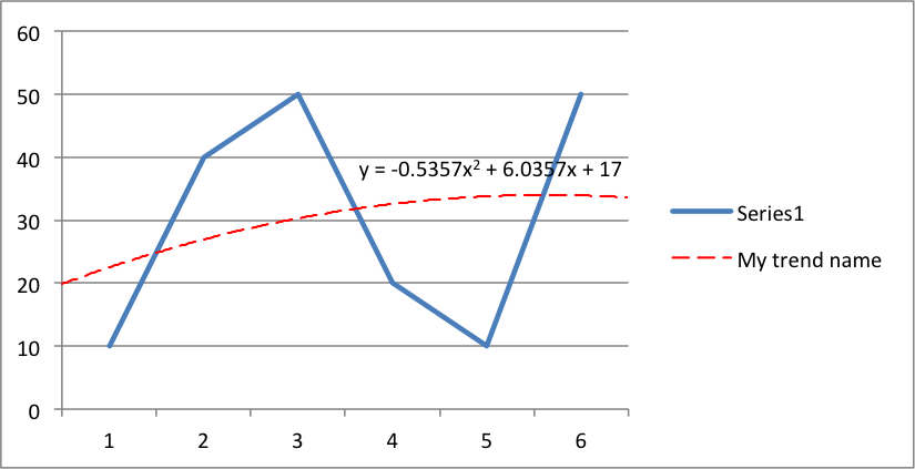
The name property sets an optional name for the trendline that will appear
in the chart legend. If it isn’t specified the Excel default name will be
displayed. This is usually a combination of the trendline type and the series
name:

chart.add_series({
    'values': '=Sheet1!$A$1:$A$6',
    'trendline': {
        'type': 'polynomial',
        'name': 'My trend name',
        'order': 2,
    },
})

The intercept property sets the point where the trendline crosses the Y
(value) axis:

chart.add_series({
    'values': '=Sheet1!$B$1:$B$6',
    'trendline': {'type': 'linear',
                  'intercept': 0.8,
    },
})

The display_equation property displays the trendline equation on the
chart:

chart.add_series({
    'values': '=Sheet1!$B$1:$B$6',
    'trendline': {'type': 'linear',
                  'display_equation': True,
    },
})

The display_r_squared property displays the R squared value of the
trendline on the chart:

chart.add_series({
    'values': '=Sheet1!$B$1:$B$6',
    'trendline': {'type': 'linear',
                  'display_r_squared': True,
    },
})

Several of these properties can be set in one go:

chart.add_series({
    'values': '=Sheet1!$A$1:$A$6',
    'trendline': {
        'type': 'polynomial',
        'name': 'My trend name',
        'order': 2,
        'forward': 0.5,
        'backward': 0.5,
        'display_equation': True,
        'line': {
            'color': 'red',
            'width': 1,
            'dash_type': 'long_dash',
        },
    },
})

Trendlines cannot be added to series in a stacked chart or pie chart, doughnut
chart, radar chart or (when implemented) to 3D or surface charts.

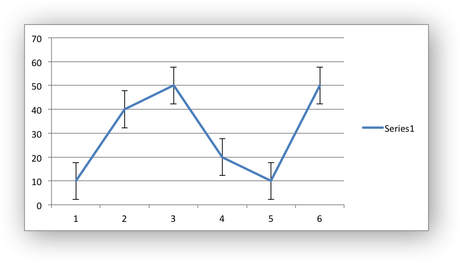
Chart series option: Error Bars

Error bars can be added to a chart series to indicate error bounds in the data.
The error bars can be vertical y_error_bars (the most common type) or
horizontal x_error_bars (for Bar and Scatter charts only).

The following properties can be set for error bars in a chart series:

type
value        (for all types except standard error and custom)
plus_values  (for custom only)
minus_values (for custom only)
direction
end_style
line

The type property sets the type of error bars in the series:

chart.add_series({
    'values':       '=Sheet1!$A$1:$A$6',
    'y_error_bars': {'type': 'standard_error'},
})

The available error bars types are available:

fixed
percentage
standard_deviation
standard_error
custom

All error bar types, except for standard_error and custom must also
have a value associated with it for the error bounds:

chart.add_series({
    'values': '=Sheet1!$A$1:$A$6',
    'y_error_bars': {
        'type': 'percentage',
        'value': 5,
    },
})

The custom error bar type must specify plus_values and minus_values
which should either by a Sheet1!$A$1:$A$6 type range formula or a list of
values:

chart.add_series({
    'categories': '=Sheet1!$A$1:$A$6',
    'values':     '=Sheet1!$B$1:$B$6',
    'y_error_bars': {
        'type':         'custom',
        'plus_values':  '=Sheet1!$C$1:$C$6',
        'minus_values': '=Sheet1!$D$1:$D$6',
    },
})

# or

chart.add_series({
    'categories': '=Sheet1!$A$1:$A$6',
    'values':     '=Sheet1!$B$1:$B$6',
    'y_error_bars': {
        'type':         'custom',
        'plus_values':  [1, 1, 1, 1, 1],
        'minus_values': [2, 2, 2, 2, 2],
    },
})

Note, as in Excel the items in the minus_values do not need to be negative.

The direction property sets the direction of the error bars. It should be
one of the following:

plus   # Positive direction only.
minus  # Negative direction only.
both   # Plus and minus directions, The default.

The end_style property sets the style of the error bar end cap. The options
are 1 (the default) or 0 (for no end cap):

chart.add_series({
    'values': '=Sheet1!$A$1:$A$6',
    'y_error_bars': {
        'type': 'fixed',
        'value': 2,
        'end_style': 0,
        'direction': 'minus'
    },
})

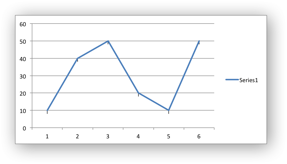
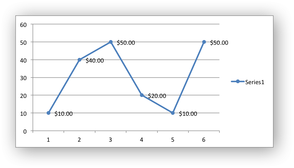
Chart series option: Data Labels

Data labels can be added to a chart series to indicate the values of the
plotted data points.

The following properties can be set for data_labels formats in a chart:

value
category
series_name
position
leader_lines
percentage
separator
legend_key
num_format
font
border
fill
pattern
gradient
custom

The value property turns on the Value data label for a series:

chart.add_series({
    'values':      '=Sheet1!$A$1:$A$6',
    'data_labels': {'value': True},
})

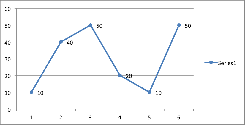
By default data labels are displayed in Excel with only the values
shown. However, it is possible to configure other display options, as shown
below.

The category property turns on the Category Name data label for a series:

chart.add_series({
    'values':      '=Sheet1!$A$1:$A$6',
    'data_labels': {'category': True},
})

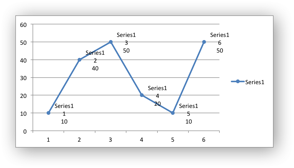
The series_name property turns on the Series Name data label for a
series:

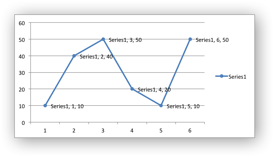
chart.add_series({
    'values':      '=Sheet1!$A$1:$A$6',
    'data_labels': {'series_name': True},
})

Here is an example with all three data label types shown:

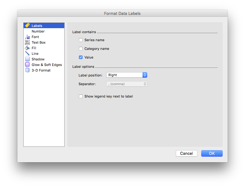
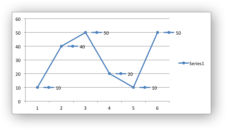
The position property is used to position the data label for a series:

chart.add_series({
    'values':      '=Sheet1!$A$1:$A$6',
    'data_labels': {'series_name': True, 'position': 'above'},
})

In Excel the allowable data label positions vary for different chart types.
The allowable positions are:

Position	Line, Scatter, Stock	Bar, Column	Pie, Doughnut	Area, Radar
center	Yes	Yes	Yes	Yes*
right	Yes*
left	Yes
above	Yes
below	Yes
inside_base		Yes
inside_end		Yes	Yes
outside_end		Yes*	Yes
best_fit			Yes*

Note: The * indicates the default position for each chart type in Excel, if
a position isn’t specified by the user.

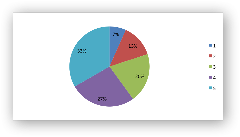
The percentage property is used to turn on the display of data labels as a
Percentage for a series. In Excel the percentage data label option is
only available for Pie and Doughnut chart variants:

chart.add_series({
    'values':      '=Sheet1!$A$1:$A$6',
    'data_labels': {'percentage': True},
})

The leader_lines property is used to turn on Leader Lines for the data
label of a series. It is mainly used for pie charts:

chart.add_series({
    'values':      '=Sheet1!$A$1:$A$6',
    'data_labels': {'value': True, 'leader_lines': True},
})

Note

Even when leader lines are turned on they aren’t automatically visible in
Excel or XlsxWriter. Due to an Excel limitation (or design) leader lines
only appear if the data label is moved manually or if the data labels are
very close and need to be adjusted automatically.

The separator property is used to change the separator between multiple
data label items:

chart.add_series({
    'values':      '=Sheet1!$A$1:$A$6',
    'data_labels': {'value': True, 'category': True,
                    'series_name': True, 'separator': "n"},
})

The separator value must be one of the following strings:

The legend_key property is used to turn on the Legend Key for the data
label of a series:

chart.add_series({
    'values':      '=Sheet1!$A$1:$A$6',
    'data_labels': {'value': True, 'legend_key': True},
})

The num_format property is used to set the number format for the data
labels of a series:

chart.add_series({
    'values':      '=Sheet1!$A$1:$A$6',
    'data_labels': {'value': True, 'num_format': '#,##0.00'},
})

The number format is similar to the Worksheet Cell Format num_format
apart from the fact that a format index cannot be used. An explicit format
string must be used as shown above. See set_num_format() for more
information.

The font property is used to set the font of the data labels of a series:

chart.add_series({
    'values': '=Sheet1!$A$1:$A$6',
    'data_labels': {
        'value': True,
        'font': {'name': 'Consolas', 'color': 'red'}
    },
})

The font property is also used to rotate the data labels of a series:

chart.add_series({

    'values': '=Sheet1!$A$1:$A$6',
    'data_labels': {
        'value': True,
        'font': {'rotation': 45}
    },
})

See Chart Fonts.

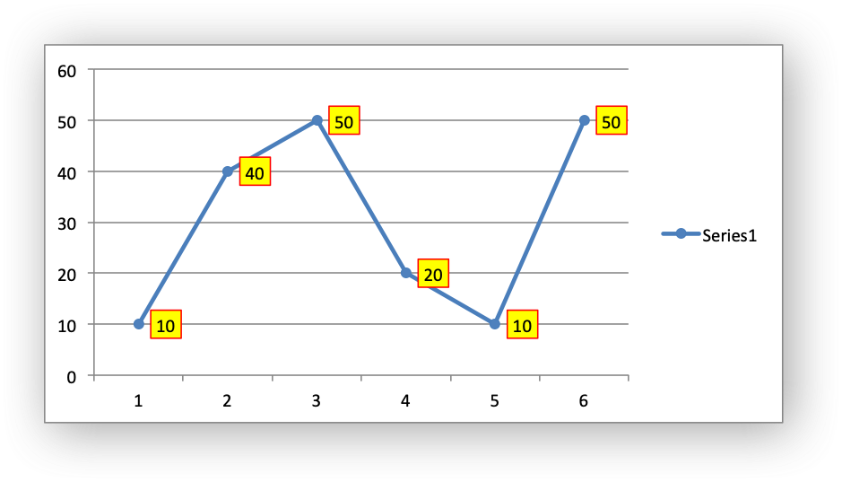
Standard chart formatting such as border and fill can also be added to
the data labels:

chart.add_series({
    'values':     '=Sheet1!$A$1:$A$6',
    'data_labels': {'value': True,
                    'border': {'color': 'red'},
                    'fill':   {'color': 'yellow'}},
})

The custom property is used to set properties for individual data
labels. This is explained in detail in the next section.

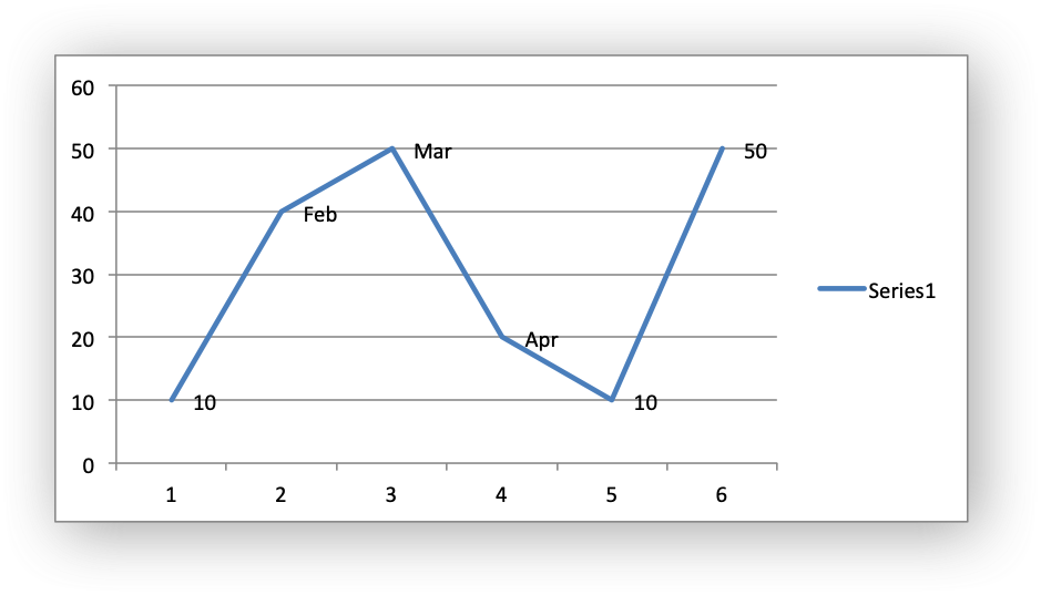
Chart series option: Custom Data Labels

The custom data label property is used to set the properties of individual
data labels in a series. The most common use for this is to set custom text or
number labels:

custom_labels = [
    {'value': 'Jan'},
    {'value': 'Feb'},
    {'value': 'Mar'},
    {'value': 'Apr'},
    {'value': 'May'},
    {'value': 'Jun'},
]

chart.add_series({
    'values': '=Sheet1!$A$1:$A$6',
    'data_labels': {'value': True, 'custom': custom_labels},
})

As shown in the previous examples th custom property should be a list of
dicts. Any property dict that is set to None or not included in the list
will be assigned the default data label value:

custom_labels = [
    None,
    {'value': 'Feb'},
    {'value': 'Mar'},
    {'value': 'Apr'},
]

chart.add_series({
    'values': '=Sheet1!$A$1:$A$6',
    'data_labels': {'value': True, 'custom': custom_labels},
})

The property elements of the custom lists should be dicts with the
following allowable keys/sub-properties:

The value property should be a string, number or formula string that refers to
a cell from which the value will be taken:

custom_labels = [
    {'value': '=Sheet1!$C$1'},
    {'value': '=Sheet1!$C$2'},
    {'value': '=Sheet1!$C$3'},
    {'value': '=Sheet1!$C$4'},
    {'value': '=Sheet1!$C$5'},
    {'value': '=Sheet1!$C$6'},
]

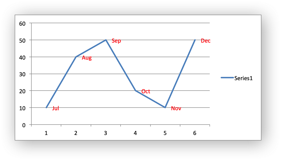
The font property is used to set the font of the custom data label of a series:

custom_labels = [
    {'value': '=Sheet1!$C$1', 'font': {'color': 'red'}},
    {'value': '=Sheet1!$C$2', 'font': {'color': 'red'}},
    {'value': '=Sheet1!$C$3', 'font': {'color': 'red'}},
    {'value': '=Sheet1!$C$4', 'font': {'color': 'red'}},
    {'value': '=Sheet1!$C$5', 'font': {'color': 'red'}},
    {'value': '=Sheet1!$C$6', 'font': {'color': 'red'}},
]

chart.add_series({
    'values': '=Sheet1!$A$1:$A$6',
    'data_labels': {'value': True, 'custom': custom_labels},
})

See Chart Fonts for details on the available font properties.

The delete property can be used to delete labels in a series. This can be
useful if you want to highlight one or more cells in the series, for example
the maximum and the minimum:

custom_labels = [
    None,
    {'delete': True},
    {'delete': True},
    {'delete': True},
    {'delete': True},
    None,
]

chart.add_series({
    'values': '=Sheet1!$A$1:$A$6',
    'data_labels': {'value': True, 'custom': custom_labels},
})

Standard chart formatting such as border and fill can also be added to
the custom data labels:

custom_labels = [
    {'value': 'Jan', 'border': {'color': 'blue'}},
    {'value': 'Feb'},
    {'value': 'Mar'},
    {'value': 'Apr'},
    {'value': 'May'},
    {'value': 'Jun', 'fill':   {'color': 'green'}},
]

chart.add_series({
    'values':     '=Sheet1!$A$1:$A$6',
    'marker': {'type': 'circle'},
    'data_labels': {'value': True,
                    'custom': custom_labels,
                    'border': {'color': 'red'},
                    'fill':   {'color': 'yellow'}},
})

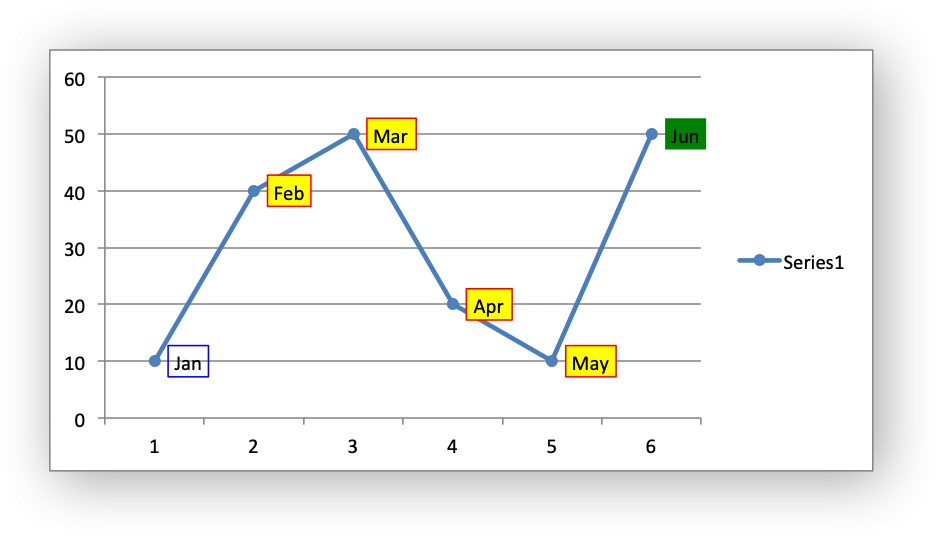
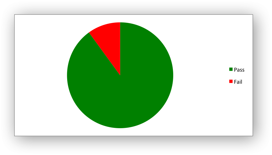
Chart series option: Points

In general formatting is applied to an entire series in a chart. However, it
is occasionally required to format individual points in a series. In
particular this is required for Pie/Doughnut charts where each segment is
represented by a point.

In these cases it is possible to use the points property of
add_series():

import xlsxwriter

workbook = xlsxwriter.Workbook('chart_pie.xlsx')

worksheet = workbook.add_worksheet()
chart = workbook.add_chart({'type': 'pie'})

data = [
    ['Pass', 'Fail'],
    [90, 10],
]

worksheet.write_column('A1', data[0])
worksheet.write_column('B1', data[1])

chart.add_series({
    'categories': '=Sheet1!$A$1:$A$2',
    'values':     '=Sheet1!$B$1:$B$2',
    'points': [
        {'fill': {'color': 'green'}},
        {'fill': {'color': 'red'}},
    ],
})

worksheet.insert_chart('C3', chart)

workbook.close()

The points property takes a list of format options (see the “Chart
Formatting” section below). To assign default properties to points in a series
pass None values in the array ref:

# Format point 3 of 3 only.
chart.add_series({
    'values': '=Sheet1!A1:A3',
    'points': [
        None,
        None,
        {'fill': {'color': '#990000'}},
    ],
})

# Format point 1 of 3 only.
chart.add_series({
    'values': '=Sheet1!A1:A3',
    'points': [
        {'fill': {'color': '#990000'}},
    ],
})

Chart series option: Smooth

The smooth option is used to set the smooth property of a line series. It
is only applicable to the line and scatter chart types:

chart.add_series({
    'categories': '=Sheet1!$A$1:$A$6',
    'values':     '=Sheet1!$B$1:$B$6',
    'smooth':     True,
})

Chart Formatting

The following chart formatting properties can be set for any chart object that
they apply to (and that are supported by XlsxWriter) such as chart lines,
column fill areas, plot area borders, markers, gridlines and other chart
elements:

line
border
fill
pattern
gradient

Chart formatting properties are generally set using dicts:

chart.add_series({
    'values': '=Sheet1!$A$1:$A$6',
    'line':   {'color': 'red'},
})

In some cases the format properties can be nested. For example a marker may
contain border and fill sub-properties:

chart.add_series({
    'values': '=Sheet1!$A$1:$A$6',
    'line':   {'color': 'blue'},
    'marker': {'type': 'square',
               'size,': 5,
               'border': {'color': 'red'},
               'fill':   {'color': 'yellow'}
    },
})

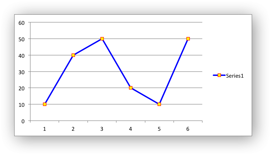
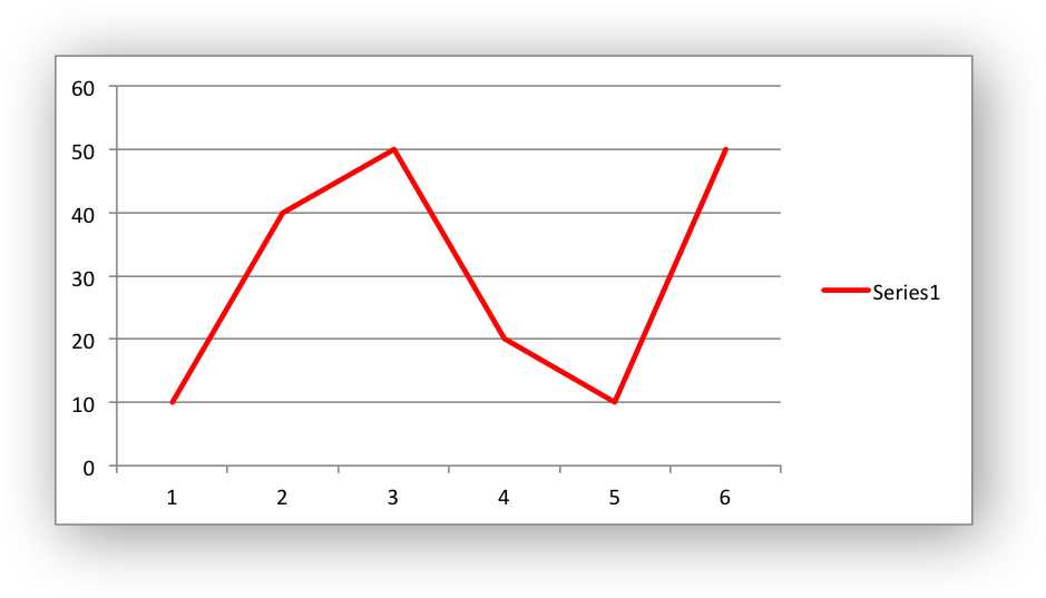
Chart formatting: Line

The line format is used to specify properties of line objects that appear in a
chart such as a plotted line on a chart or a border.

The following properties can be set for line formats in a chart:

none
color
width
dash_type
transparency

The none property is used to turn the line off (it is always on by
default except in Scatter charts). This is useful if you wish to plot a series
with markers but without a line:

chart.add_series({
    'values': '=Sheet1!$A$1:$A$6',
    'line':   {'none': True},
    'marker': {'type': 'automatic'},
})

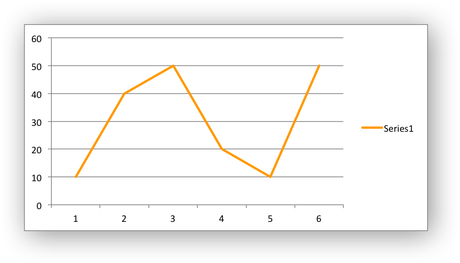
The color property sets the color of the line:

chart.add_series({
    'values': '=Sheet1!$A$1:$A$6',
    'line':   {'color': 'red'},
})

The available colors are shown in the main XlsxWriter documentation. It is
also possible to set the color of a line with a Html style #RRGGBB string
or a limited number of named colors, see Working with Colors:

chart.add_series({
    'values': '=Sheet1!$A$1:$A$6',
    'line':   {'color': '#FF9900'},
})

The width property sets the width of the line. It should be specified
in increments of 0.25 of a point as in Excel:

chart.add_series({
    'values': '=Sheet1!$A$1:$A$6',
    'line':   {'width': 3.25},
})

The dash_type property sets the dash style of the line:

chart.add_series({
    'values': '=Sheet1!$A$1:$A$6',
    'line':   {'dash_type': 'dash_dot'},
})

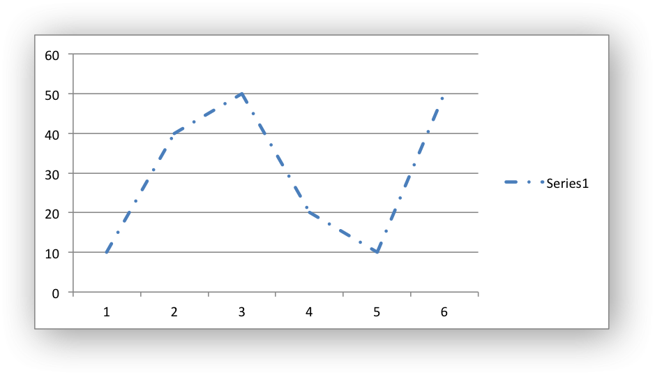
The following dash_type values are available. They are shown in the order
that they appear in the Excel dialog:

solid
round_dot
square_dot
dash
dash_dot
long_dash
long_dash_dot
long_dash_dot_dot

The default line style is solid.

The transparency property sets the transparency of the line color in the
integer range 1 — 100. The color must be set for transparency to work, it
doesn’t work with an automatic/default color:

chart.add_series({
    'values': '=Sheet1!$A$1:$A$6',
    'line':   {'color': 'yellow', 'transparency': 50},
})

More than one line property can be specified at a time:

chart.add_series({
    'values': '=Sheet1!$A$1:$A$6',
     'line': {
         'color': 'red',
         'width': 1.25,
         'dash_type': 'square_dot',
     },
})

Chart formatting: Border

The border property is a synonym for line.

It can be used as a descriptive substitute for line in chart types such as
Bar and Column that have a border and fill style rather than a line style. In
general chart objects with a border property will also have a fill
property.

Chart formatting: Solid Fill

The solid fill format is used to specify filled areas of chart objects such as
the interior of a column or the background of the chart itself.

The following properties can be set for fill formats in a chart:

The none property is used to turn the fill property off (it is
generally on by default):

chart.add_series({
    'values': '=Sheet1!$A$1:$A$6',
    'fill':   {'none': True},
    'border': {'color': 'black'}
})

The color property sets the color of the fill area:

chart.add_series({
    'values': '=Sheet1!$A$1:$A$6',
    'fill':   {'color': 'red'}
})

The available colors are shown in the main XlsxWriter documentation. It is
also possible to set the color of a fill with a Html style #RRGGBB string
or a limited number of named colors, see Working with Colors:

chart.add_series({
    'values': '=Sheet1!$A$1:$A$6',
    'fill':   {'color': '#FF9900'}
})

The transparency property sets the transparency of the solid fill color in
the integer range 1 — 100. The color must be set for transparency to work, it
doesn’t work with an automatic/default color:

chart.set_chartarea({'fill': {'color': 'yellow', 'transparency': 50}})

The fill format is generally used in conjunction with a border format
which has the same properties as a line format:

chart.add_series({
    'values': '=Sheet1!$A$1:$A$6',
    'fill':   {'color': 'red'},
    'border': {'color': 'black'}
})

Chart formatting: Pattern Fill

The pattern fill format is used to specify pattern filled areas of chart
objects such as the interior of a column or the background of the chart
itself.

The following properties can be set for pattern fill formats in a chart:

pattern:   the pattern to be applied (required)
fg_color:  the foreground color of the pattern (required)
bg_color:  the background color (optional, defaults to white)

For example:

chart.set_plotarea({
    'pattern': {
        'pattern': 'percent_5',
        'fg_color': 'red',
        'bg_color': 'yellow',
    }
})

The following patterns can be applied:

percent_5
percent_10
percent_20
percent_25
percent_30
percent_40
percent_50
percent_60
percent_70
percent_75
percent_80
percent_90
light_downward_diagonal
light_upward_diagonal
dark_downward_diagonal
dark_upward_diagonal
wide_downward_diagonal
wide_upward_diagonal
light_vertical
light_horizontal
narrow_vertical
narrow_horizontal
dark_vertical
dark_horizontal
dashed_downward_diagonal
dashed_upward_diagonal
dashed_horizontal
dashed_vertical
small_confetti
large_confetti
zigzag
wave
diagonal_brick
horizontal_brick
weave
plaid
divot
dotted_grid
dotted_diamond
shingle
trellis
sphere
small_grid
large_grid
small_check
large_check
outlined_diamond
solid_diamond

The foreground color, fg_color, is a required parameter and can be a Html
style #RRGGBB string or a limited number of named colors, see
Working with Colors.

The background color, bg_color, is optional and defaults to white.

If a pattern fill is used on a chart object it overrides the solid fill
properties of the object.

Chart formatting: Gradient Fill

The gradient fill format is used to specify gradient filled areas of chart
objects such as the interior of a column or the background of the chart
itself.

The following properties can be set for gradient fill formats in a chart:

colors:    a list of colors
positions: an optional list of positions for the colors
type:      the optional type of gradient fill
angle:     the optional angle of the linear fill

The colors property sets a list of colors that define the gradient:

chart.set_plotarea({
    'gradient': {'colors': ['#FFEFD1', '#F0EBD5', '#B69F66']}
})

Excel allows between 2 and 10 colors in a gradient but it is unlikely that
you will require more than 2 or 3.

As with solid or pattern fill it is also possible to set the colors of a
gradient with a Html style #RRGGBB string or a limited number of named
colors, see Working with Colors:

chart.add_series({
    'values':   '=Sheet1!$A$1:$A$6',
    'gradient': {'colors': ['red', 'green']}
})

The positions defines an optional list of positions, between 0 and 100, of
where the colors in the gradient are located. Default values are provided for
colors lists of between 2 and 4 but they can be specified if required:

chart.add_series({
    'values': '=Sheet1!$A$1:$A$6',
    'gradient': {
        'colors':    ['#DDEBCF', '#156B13'],
        'positions': [10,        90],
    }
})

The type property can have one of the following values:

linear        (the default)
radial
rectangular
path

For example:

chart.add_series({
    'values': '=Sheet1!$A$1:$A$6',
    'gradient': {
        'colors': ['#DDEBCF', '#9CB86E', '#156B13'],
        'type': 'radial'
    }
})

If type isn’t specified it defaults to linear.

For a linear fill the angle of the gradient can also be specified:

chart.add_series({
    'values': '=Sheet1!$A$1:$A$6',
    'gradient': {'colors': ['#DDEBCF', '#9CB86E', '#156B13'],
                 'angle': 45}
})

The default angle is 90 degrees.

If gradient fill is used on a chart object it overrides the solid fill and
pattern fill properties of the object.

Chart Fonts

The following font properties can be set for any chart object that they apply
to (and that are supported by XlsxWriter) such as chart titles, axis labels,
axis numbering and data labels:

name
size
bold
italic
underline
rotation
color

These properties correspond to the equivalent Worksheet cell Format object
properties. See the The Format Class section for more details about Format
properties and how to set them.

The following explains the available font properties:

name: Set the font name:

chart.set_x_axis({'num_font':  {'name': 'Arial'}})

size: Set the font size:

chart.set_x_axis({'num_font':  {'name': 'Arial', 'size': 9}})

bold: Set the font bold property:

chart.set_x_axis({'num_font':  {'bold': True}})

italic: Set the font italic property:

chart.set_x_axis({'num_font':  {'italic': True}})

underline: Set the font underline property:

chart.set_x_axis({'num_font':  {'underline': True}})

rotation: Set the font rotation, angle, property in the integer
range -90 to 90 deg, and 270-271 deg:
```
chart.set_x_axis({'num_font':  {'rotation': 45}})
```
The font rotation angle is useful for displaying axis data such as dates in
a more compact format.

There are 2 special case angles outside the range -90 to 90:
- 270: Stacked text, where the text runs from top to bottom.
- 271: A special variant of stacked text for East Asian fonts.

color: Set the font color property. Can be a color index, a color name
or HTML style RGB color:

chart.set_x_axis({'num_font': {'color': 'red' }})
chart.set_y_axis({'num_font': {'color': '#92D050'}})

Here is an example of Font formatting in a Chart program:

chart.set_title({
    'name': 'Test Results',
    'name_font': {
        'name': 'Calibri',
        'color': 'blue',
    },
})

chart.set_x_axis({
    'name': 'Month',
    'name_font': {
        'name': 'Courier New',
        'color': '#92D050'
    },
    'num_font': {
        'name': 'Arial',
        'color': '#00B0F0',
    },
})

chart.set_y_axis({
    'name': 'Units',
    'name_font': {
        'name': 'Century',
        'color': 'red'
    },
    'num_font': {
        'bold': True,
        'italic': True,
        'underline': True,
        'color': '#7030A0',
    },
})

chart.set_legend({'font': {'bold': 1, 'italic': 1}})

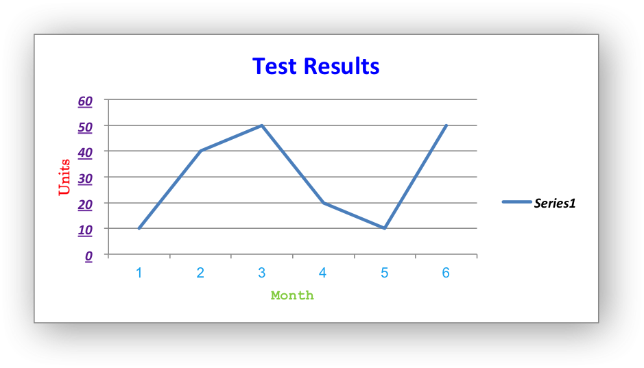
Chart Layout

The position of the chart in the worksheet is controlled by the
set_size() method.

It is also possible to change the layout of the following chart sub-objects:

plotarea
legend
title
x_axis caption
y_axis caption

Here are some examples:

chart.set_plotarea({
    'layout': {
        'x':      0.13,
        'y':      0.26,
        'width':  0.73,
        'height': 0.57,
    }
})

chart.set_legend({
    'layout': {
        'x':      0.80,
        'y':      0.37,
        'width':  0.12,
        'height': 0.25,
    }
})

chart.set_title({
    'name':    'Title',
    'overlay': True,
    'layout': {
        'x': 0.42,
        'y': 0.14,
    }
})

chart.set_x_axis({
    'name': 'X axis',
    'name_layout': {
        'x': 0.34,
        'y': 0.85,
    }
})

See set_plotarea(), set_legend(), set_title() and
set_x_axis(),

Note

It is only possible to change the width and height for the plotarea
and legend objects. For the other text based objects the width and
height are changed by the font dimensions.

The layout units must be a float in the range 0 < x <= 1 and are expressed
as a percentage of the chart dimensions as shown below:

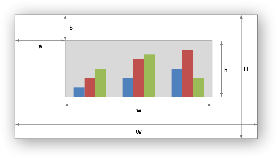
From this the layout units are calculated as follows:

layout:
    x      = a / W
    y      = b / H
    width  = w / W
    height = h / H

These units are cumbersome and can vary depending on other elements in the
chart such as text lengths. However, these are the units that are required by
Excel to allow relative positioning. Some trial and error is generally
required.

Note

The plotarea origin is the top left corner in the plotarea itself and
does not take into account the axes.

Date Category Axes

Date Category Axes are category axes that display time or date information. In
XlsxWriter Date Category Axes are set using the date_axis option in
set_x_axis() or set_y_axis():

chart.set_x_axis({'date_axis': True})

In general you should also specify a number format for a date axis although
Excel will usually default to the same format as the data being plotted:

chart.set_x_axis({
    'date_axis':  True,
    'num_format': 'dd/mm/yyyy',
})

Excel doesn’t normally allow minimum and maximum values to be set for category
axes. However, date axes are an exception. The min and max values
should be set as Excel times or dates:

chart.set_x_axis({
    'date_axis': True,
    'min': date(2013, 1, 2),
    'max': date(2013, 1, 9),
    'num_format': 'dd/mm/yyyy',
})

For date axes it is also possible to set the type of the major and minor units:

chart.set_x_axis({
    'date_axis':       True,
    'minor_unit':      4,
    'minor_unit_type': 'months',
    'major_unit':      1,
    'major_unit_type': 'years',
    'num_format':      'dd/mm/yyyy',
})

See Example: Date Axis Chart.

Chart Secondary Axes

It is possible to add a secondary axis of the same type to a chart by setting
the y2_axis or x2_axis property of the series:

import xlsxwriter

workbook = xlsxwriter.Workbook('chart_secondary_axis.xlsx')
worksheet = workbook.add_worksheet()

data = [
    [2, 3, 4, 5, 6, 7],
    [10, 40, 50, 20, 10, 50],
]

worksheet.write_column('A2', data[0])
worksheet.write_column('B2', data[1])

chart = workbook.add_chart({'type': 'line'})

# Configure a series with a secondary axis.
chart.add_series({
    'values': '=Sheet1!$A$2:$A$7',
    'y2_axis': True,
})

# Configure a primary (default) Axis.
chart.add_series({
    'values': '=Sheet1!$B$2:$B$7',
})

chart.set_legend({'position': 'none'})

chart.set_y_axis({'name': 'Primary Y axis'})
chart.set_y2_axis({'name': 'Secondary Y axis'})

worksheet.insert_chart('D2', chart)

workbook.close()

It is also possible to have a secondary, combined, chart either with a shared
or secondary axis, see below.

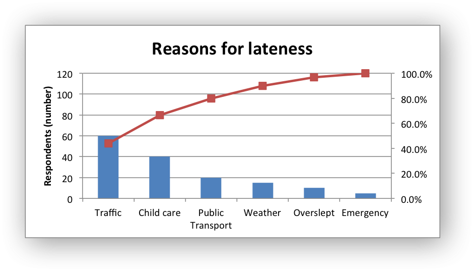
Combined Charts

It is also possible to combine two different chart types, for example a column
and line chart to create a Pareto chart using the Chart combine()
method:

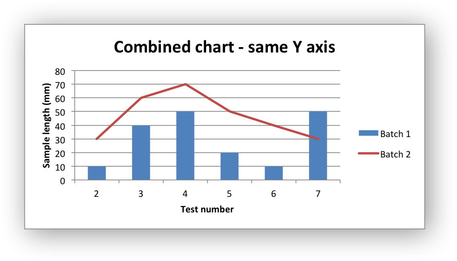
The combined charts can share the same Y axis like the following example:

# Usual setup to create workbook and add data...

# Create a new column chart. This will use this as the primary chart.
column_chart = workbook.add_chart({'type': 'column'})

# Configure the data series for the primary chart.
column_chart.add_series({
    'name':       '=Sheet1!B1',
    'categories': '=Sheet1!A2:A7',
    'values':     '=Sheet1!B2:B7',
})

# Create a new column chart. This will use this as the secondary chart.
line_chart = workbook.add_chart({'type': 'line'})

# Configure the data series for the secondary chart.
line_chart.add_series({
    'name':       '=Sheet1!C1',
    'categories': '=Sheet1!A2:A7',
    'values':     '=Sheet1!C2:C7',
})

# Combine the charts.
column_chart.combine(line_chart)

# Add a chart title and some axis labels. Note, this is done via the
# primary chart.
column_chart.set_title({ 'name': 'Combined chart - same Y axis'})
column_chart.set_x_axis({'name': 'Test number'})
column_chart.set_y_axis({'name': 'Sample length (mm)'})

# Insert the chart into the worksheet
worksheet.insert_chart('E2', column_chart)

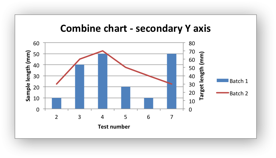
The secondary chart can also be placed on a secondary axis using the methods
shown in the previous section.

In this case it is just necessary to add a y2_axis parameter to the series
and, if required, add a title using set_y2_axis(). The following are
the additions to the previous example to place the secondary chart on the
secondary axis:

# ...
line_chart.add_series({
    'name':       '=Sheet1!C1',
    'categories': '=Sheet1!A2:A7',
    'values':     '=Sheet1!C2:C7',
    'y2_axis':    True,
})

# Add a chart title and some axis labels.
# ...
column_chart.set_y2_axis({'name': 'Target length (mm)'})

The examples above use the concept of a primary and secondary chart. The
primary chart is the chart that defines the primary X and Y axis. It is also
used for setting all chart properties apart from the secondary data
series. For example the chart title and axes properties should be set via the
primary chart.

See also Example: Combined Chart and Example: Pareto Chart for more detailed
examples.

There are some limitations on combined charts:

Only two charts can be combined.
Pie charts cannot currently be combined.
Scatter charts cannot currently be used as a primary chart but they can be
used as a secondary chart.
Bar charts can only combined secondary charts on a secondary axis. This is
an Excel limitation.

Chartsheets

The examples shown above and in general the most common type of charts in Excel
are embedded charts.

However, it is also possible to create “Chartsheets” which are worksheets that
are comprised of a single chart:

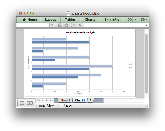
See The Chartsheet Class for details.

Charts from Worksheet Tables

Charts can by created from Worksheet Tables. However, Excel
has a limitation where the data series name, if specified, must refer to a
cell within the table (usually one of the headers).

To workaround this Excel limitation you can specify a user defined name in the
table and refer to that from the chart:

import xlsxwriter

workbook = xlsxwriter.Workbook('chart_pie.xlsx')

worksheet = workbook.add_worksheet()

data = [
    ['Apple',  60],
    ['Cherry', 30],
    ['Pecan',  10],
]

worksheet.add_table('A1:B4', {'data': data,
                              'columns': [{'header': 'Types'},
                                         {'header': 'Number'}]}
)

chart = workbook.add_chart({'type': 'pie'})

chart.add_series({
    'name':       '=Sheet1!$A$1',
    'categories': '=Sheet1!$A$2:$A$4',
    'values':     '=Sheet1!$B$2:$B$4',
})

worksheet.insert_chart('D2', chart)

workbook.close()

Chart Limitations

The following chart features aren’t supported in XlsxWriter:

3D charts and controls.
Bubble, Surface or other chart types not listed in The Chart Class.

Источник

Диаграммы — отличный способ быстро визуализировать и понять огромное количество данных. Существует множество различных типов диаграмм: столбчатая диаграмма, линейная диаграмма, круговая диаграмма, и так далее. Модуль openpyxl поддерживает многие из них.

Здесь будут разбираться приемы создания наиболее часто используемых диаграмм — это столбчатая и линейная диаграммы. Так как теория лежащая в основе создания диаграмм одинакова, создание остальных типов диаграмм не составит труда.

Примечание: В зависимости от того, что используется для просмотра документа XLSX — Microsoft Excel или альтернатива с открытым исходным кодом (LibreOffice Calc или OpenOffice Calc), диаграмма может выглядеть немного иначе. В частности, LibreOffice Calc неправильно отображает подписи осей, заголовок диаграммы вообще не выводится. Кстати китайский WPS Office Calc отображает все корректно.

Содержание:

Основы построения диаграмм.
Создание столбчатых гистограмм.
- 3D столбчатые гистограммы.
Создание линейных диаграмм.
- 3D линейные диаграммы.
Таблицы диаграмм XLSX-документа.
Отображение определенных регионов на диаграмме.

Основы построения диаграмм.

Диаграммы состоят, по крайней мере, из одного или нескольких рядов данных. Сами ряды данных состоят из ссылок на диапазоны ячеек.

from openpyxl import Workbook
from openpyxl.chart import BarChart, Reference

wb = Workbook()
ws = wb.active

# данные для диаграммы
data = [
    ["Product", "Online", "Store"],
    [1, 30, 45],
    [2, 40, 30],
    [3, 40, 25],
    [4, 50, 30],
    [5, 30, 25],
    [6, 25, 35],
    [7, 20, 40],
]
for row in data:
    ws.append(row)

# выбираем диапазоны значений для диаграммы
values = Reference(worksheet=ws,
                 min_row=1,
                 max_row=8,
                 min_col=2,
                 max_col=3)
# создаем объект столбчатой диаграммы
chart = BarChart()
# добавляем в диаграмму выбранный диапазон значений
chart.add_data(values, titles_from_data=True)
# привязываем диаграмму к ячейке `E15`
ws.add_chart(chart, "A11")
# определяем размеры диаграммы в сантиметрах
chart.width = 20
chart.height = 5
# сохраняем и смотрим что получилось
wb.save("sample-chart.xlsx")

По умолчанию верхний левый угол диаграммы привязан к ячейке 'A11' и имеет размер 15 x 7,5 см. Размеры диаграммы можно изменить, задав нижеуказанные свойства:

chart.width — ширина диаграммы, по умолчанию 15 сантиметров.
chart.heigh — высота диаграммы, по умолчанию 7,5 сантиметров.

Внимание. Фактический размер будет зависеть от операционной системы и устройства.

Создание столбчатых гистограмм.

На столбчатых гистограммах, значения отображаются либо в виде горизонтальных полос, либо в виде вертикальных столбцов.

Следующие настройки влияют на вид столбчатых гистограмм:

Для переключения между вертикальной и горизонтальной гистограммами, необходимо просто изменить ее тип .type = "col" (вертикальные столбцы) или .type = "bar" (горизонтальные полосы).
При использовании диаграмм с накоплением, для свойства .overlap необходимо установить значение 100.
Если диаграмма имеет вид горизонтальных полос, то оси x и y меняются местами.
Свойство объекта диаграммы .grouping может принимать одно из значений: 'percentStacked', 'stacked', 'standard' (по умолчанию).

Смотрим пример четырех гистограмм, который иллюстрирует различные возможности и настройки (с подробным описанием кода):

from copy import deepcopy
from openpyxl import Workbook
from openpyxl.chart import BarChart, Reference

wb = Workbook()
ws = wb.active

# данные для построения диаграмм
rows = [
    ('Number', 'Batch 1', 'Batch 2'),
    (2, 10, 30),
    (3, 40, 60),
    (4, 50, 70),
    (5, 20, 10),
    (6, 10, 40),
    (7, 50, 30),
]
for row in rows:
    ws.append(row)

# ДИАГРАММА №1
# создаем объект диаграммы
chart1 = BarChart()
# установим тип - `вертикальные столбцы`
chart1.type = "col"
# установим стиль диаграммы (цветовая схема)
chart1.style = 10
# заголовок диаграммы
chart1.title = "Столбчатая диаграмма"
# подпись оси `y`
chart1.y_axis.title = 'Длина выборки'
# показывать данные на оси (для LibreOffice Calc)
chart1.y_axis.delete = False
# подпись оси `x`
chart1.x_axis.title = 'Номер теста'
chart1.x_axis.delete = False
# выберем 2 столбца с данными для оси `y`
data = Reference(ws, min_col=2, max_col=3, min_row=1, max_row=7)
# теперь выберем категорию для оси `x`
categor = Reference(ws, min_col=1, min_row=2, max_row=7)
# добавляем данные в объект диаграммы
chart1.add_data(data, titles_from_data=True)
# установим метки на объект диаграммы
chart1.set_categories(categor)
# добавим диаграмму на лист, в ячейку "A10"
ws.add_chart(chart1, "A10")

# ДИАГРАММА №2
# что бы показать типы столбчатых диаграмм, скопируем 
# первую диаграмму и будем менять настройки
chart2 = deepcopy(chart1)
# изменяем стиль
chart2.style = 11
# установим тип - `горизонтальные полосы`
chart2.type = "bar"
chart2.title = "Горизонтальные полосы"
ws.add_chart(chart2, "A25")

# ДИАГРАММА №3
chart3 = deepcopy(chart1)
chart3.type = "col"
chart3.style = 12
# зададим группировку
chart3.grouping = "stacked"
# для диаграммы с группировкой, 
# необходимо установить перекрытие
chart3.overlap = 100
chart3.title = 'Сложенная диаграмма'
ws.add_chart(chart3, "A40")

# ДИАГРАММА №4
chart4 = deepcopy(chart1)
chart4.type = "bar"
chart4.style = 13
chart4.grouping = "percentStacked"
chart4.overlap = 100
# отключим линии сетки
chart4.y_axis.majorGridlines = None
# уберем легенду
chart4.legend = None
chart4.title = 'Диаграмма с процентным накоплением'
ws.add_chart(chart4, "A55")

# сохраняем и смотрим что получилось
wb.save("bar.xlsx")

3D столбчатые гистограммы.

При помощи модуля openpyxl также можно создавать трехмерные гистограммы. Смотрим пример простой трехмерной гистограммы:

from openpyxl import Workbook
from openpyxl.chart import Reference, BarChart3D

wb = Workbook()
ws = wb.active

rows = [
    (None, 2013, 2014),
    ("Apples", 5, 4),
    ("Oranges", 6, 2),
    ("Pears", 8, 3)
]

for row in rows:
    ws.append(row)

data = Reference(ws, min_col=2, min_row=1, max_col=3, max_row=4)
titles = Reference(ws, min_col=1, min_row=2, max_row=4)
chart = BarChart3D()
chart.title = "3D Bar Chart"
chart.add_data(data=data, titles_from_data=True)
chart.set_categories(titles)

ws.add_chart(chart, "E5")
wb.save("bar3d.xlsx")

Создание линейных диаграмм.

Линейные диаграммы позволяют отображать данные относительно фиксированной оси. Они похожи на точечные диаграммы, главное отличие состоит в том, что в линейных диаграммах каждый ряд данных отображается на основе одних и тех же значений. В качестве вспомогательных осей можно использовать различные типы осей.

Как и столбчатые гистограммы, линейные диаграммы бывают трех видов: 'standard' (стандартные), 'stacked' (с накоплением) и 'percentStacked' (с процентным накоплением).

Смотрим пример линейных диаграмм, который иллюстрирует различные возможности и настройки (с подробным описанием кода):

from openpyxl import Workbook
from openpyxl.chart import LineChart, Reference
from openpyxl.chart.axis import DateAxis
from datetime import date
from copy import deepcopy

wb = Workbook()
ws = wb.active

# данные для построения диаграммы
rows = [
    ['Date', 'Batch 1', 'Batch 2', 'Batch 3'],
    [date(2015,9, 1), 40, 30, 25],
    [date(2015,9, 2), 40, 25, 30],
    [date(2015,9, 3), 50, 30, 45],
    [date(2015,9, 4), 30, 25, 40],
    [date(2015,9, 5), 25, 35, 30],
    [date(2015,9, 6), 20, 40, 35],
]
for row in rows:
    ws.append(row)

# ДИАГРАММА №1
# создаем объект диаграммы
chart1 = LineChart()
# заголовок диаграммы
chart1.title = "Линейная диаграмма"
# установим цветовую схему диаграммы
chart1.style = 13
# подпись оси `y`
chart1.y_axis.title = 'Размер'
# показывать данные на оси (для LibreOffice Calc)
chart1.y_axis.delete = False
# подпись оси `x`
chart1.x_axis.title = 'Номер теста'
chart1.x_axis.delete = False
# выберем 4 столбца с данными для оси `y` 
# в итоге получим 4 графика
data = Reference(ws, min_col=2, max_col=4, min_row=1, max_row=7)
# добавляем данные в объект диаграммы
chart1.add_data(data, titles_from_data=True)
# ТЕПЕРЬ ЗАДАДИМ СТИЛЬ ЛИНИЙ 
# ЛИНИЯ С ДАННЫМИ ИЗ 1 СТОЛБЦА ДАННЫХ
line1 = chart1.series[0]
# символ маркера для текущего значения
line1.marker.symbol = "x"
# цвет заливки маркера
line1.marker.graphicalProperties.solidFill = "FF0000"
line1.marker.graphicalProperties.line.solidFill = "FF0000"
# не заливаем линию между маркерами (прозрачная)
line1.graphicalProperties.line.noFill = True
# ЛИНИЯ С ДАННЫМИ ИЗ 2 СТОЛБЦА ДАННЫХ
line2 = chart1.series[1]
# цвет заливки линии графика
line2.graphicalProperties.line.solidFill = "00AAAA"
# делаем линию пунктирной
line2.graphicalProperties.line.dashStyle = "sysDot"
# ширина указывается в EMU
line2.graphicalProperties.line.width = 100050
# ЛИНИЯ С ДАННЫМИ ИЗ 3 СТОЛБЦА ДАННЫХ
line3 = chart1.series[2]
# символ маркера для текущего значения
line3.marker.symbol = "triangle"
# покрасим маркер в другой цвет
line1.marker.graphicalProperties.solidFill = "FF0000"
line3.marker.graphicalProperties.line.solidFill = "0000FF"
# делаем линию гладкой
line3.smooth = True
# добавим диаграмму на лист, в ячейку "A10"
ws.add_chart(chart1, "A10")

# ДИАГРАММА №2
# скопируем первую диаграмму
stacked = deepcopy(chart1)
# диаграмма с накоплением
stacked.grouping = "stacked"
stacked.title = "Графики с накоплением"
ws.add_chart(stacked, "A27")

# ДИАГРАММА №3
percent_stacked = deepcopy(chart1)
# диаграмма с процентным накоплением
percent_stacked.grouping = "percentStacked"
percent_stacked.title = "Графики с процентным накоплением"
ws.add_chart(percent_stacked, "A44")

# ДИАГРАММА №4 с датами по оси `x`, все линии
# графиков будут иметь стиль по умолчанию
# создаем объект диаграммы
chart2 = LineChart()
chart2.title = "Графики с осью дат"
# установим другую цветовую схему
chart2.style = 12
# подпись оси `y`
chart2.y_axis.title = "Размер"
chart2.y_axis.delete = False
# поперечная ось
chart2.y_axis.crossAx = 500
# подпись оси `x`
chart2.x_axis.title = "Дата"
chart2.x_axis.delete = False
chart2.x_axis = DateAxis(crossAx=100)
# формат отображения дат на оси `x`
chart2.x_axis.number_format = 'd-mmm'
# задаем временную единицу даты
chart2.x_axis.majorTimeUnit = "days"
# добавляем выборку данных из первой диаграммы
chart2.add_data(data, titles_from_data=True)
# делаем выборку данных для оси `x`
dates = Reference(ws, min_col=1, min_row=2, max_row=7)
chart2.set_categories(dates)
ws.add_chart(chart2, "A61")

# сохраняем и смотрим что получилось
wb.save("line.xlsx")

Примечание:

Атрибут линии dashStyle может принимать одно из значений: ‘dot’, ‘lgDashDot’, ‘lgDashDotDot’, ‘sysDash’, ‘lgDash’, ‘sysDot’, ‘solid’ (по умолчанию), ‘dashDot’, ‘sysDashDotDot’, ‘dash’, ‘sysDashDot’
Атрибут маркера marker.symbol может принимать одно из значений: ‘dot’, ‘plus’, ‘triangle’, ‘x’, ‘star’, ‘diamond’, ‘square’, ‘circle’, ‘dash’, ‘auto’ (по умолчанию).

3D линейные диаграммы.

В трехмерных линейных диаграммах проекция третьей оси совпадает с названием столбцов выбранных данных, в общем с легендой.

from datetime import date
from openpyxl import Workbook
from openpyxl.chart import LineChart3D, Reference
from openpyxl.chart.axis import DateAxis

wb = Workbook()
ws = wb.active

rows = [
    ['Date', 'Batch 1', 'Batch 2', 'Batch 3'],
    [date(2015,9, 1), 40, 30, 25],
    [date(2015,9, 2), 40, 25, 30],
    [date(2015,9, 3), 50, 30, 45],
    [date(2015,9, 4), 30, 25, 40],
    [date(2015,9, 5), 25, 35, 30],
    [date(2015,9, 6), 20, 40, 35],
]
for row in rows:
    ws.append(row)

# создаем объект диаграммы
chart = LineChart3D()
# устанавливаем атрибуты
chart.title = "3D Линейный график"
# легенда не нужна, т.к. 3-я ось совпадает
# с названиями столбцов выборки
chart.legend = None
chart.style = 15
chart.y_axis.title = 'Размер'
chart.x_axis.title = 'Номер теста'
# делаем выборку и добавляем ее в объект диаграммы
data = Reference(ws, min_col=2, min_row=1, max_col=4, max_row=7)
chart.add_data(data, titles_from_data=True)
# добавляем диаграмму на лист в ячейку "A10"
ws.add_chart(chart, "A10")

# сохраняем и смотрим что получилось
wb.save("line3D.xlsx")

Таблицы диаграмм XLSX-документа.

Диаграммы можно добавлять в специальные рабочие листы, называемые таблицами диаграмм, которые содержат только диаграммы.

Все данные для диаграммы должны быть на другом листе электронной таблицы.

from openpyxl import Workbook
from openpyxl.chart import PieChart, Reference, Series

wb = Workbook()
ws = wb.active
# создаем таблицу диаграммы
chartsheet = wb.create_chartsheet("Круговая диаграмма")

rows = [
    ["Bob", 3],
    ["Harry", 2],
    ["James", 4],
]
for row in rows:
    ws.append(row)

# создаем rheujde. lbfuhfvve
chart = PieChart()
# выбираем данные
labels = Reference(ws, min_col=1, min_row=1, max_row=3)
data = Reference(ws, min_col=2, min_row=1, max_row=3)
# добавляем данные 
chart.add_data(data, titles_from_data=False)
chart.set_categories(labels)
chart.title = "Круговая диаграмма"
# размеры диаграммы
chart.width = 15
chart.height = 15
# добавляем на лист диаграмм
chartsheet.add_chart(chart)

wb.save("create_chartsheet.xlsx")

Отображение определенных регионов на диаграмме.

Минимальные и максимальные значения осей можно установить вручную для отображения определенных регионов на диаграмме.

from openpyxl import Workbook
from openpyxl.chart import ScatterChart, Reference, Series

wb = Workbook()
ws = wb.active

#  данные диаграммы
ws.append(['X', '1/X'])
for x in range(-10, 11):
    if x:
        ws.append([x, 1.0 / x])

# ДИАГРАММА 1
chart1 = ScatterChart()
chart1.title = "Полные Оси"
chart1.x_axis.title = 'x'
chart1.x_axis.delete = False
chart1.y_axis.title = '1/x'
chart1.y_axis.delete = False
chart1.legend = None

# ДИАГРАММА 2
chart2 = ScatterChart()
chart2.title = "Clipped Axes"
chart2.x_axis.title = 'x'
chart2.x_axis.delete = False
chart2.y_axis.title = '1/x'
chart2.y_axis.delete = False
chart2.legend = None
# устанавливаем минимумы
chart2.x_axis.scaling.min = 0
chart2.y_axis.scaling.min = 0
# устанавливаем максимумы
chart2.x_axis.scaling.max = 11
chart2.y_axis.scaling.max = 1.5
# делаем выборку 
x = Reference(ws, min_col=1, min_row=2, max_row=22)
y = Reference(ws, min_col=2, min_row=2, max_row=22)
# собираем серию
series = Series(y, xvalues=x)
# добавляем в объекты диаграмм
chart1.append(series)
chart2.append(series)
# добавляем диаграммы на лист Excel
ws.add_chart(chart1, "d1")
ws.add_chart(chart2, "d17")

wb.save("minmax.xlsx")

Примечание. В некоторых случаях, таких как в примере, установка пределов оси фактически эквивалентна отображению поддиапазона данных. Для больших наборов данных визуализация точечных диаграмм (и, возможно, других) будет намного быстрее при использовании подмножеств данных, а не ограничений по осям как в Excel, так и в OpenOffice Calc/LibreOffice Calc.

Источник

Давайте посмотрим правде в глаза. Независимо от того, чем мы занимаемся, рано или поздно нам придется иметь дело с повторяющимися задачами, такими как обновление ежедневного отчета в Excel.

Python идеально подходит для решения задач автоматизации. Но если вы работаете компании, которая не использует Python, вам будет сложно автоматизировать рабочие задачи с помощью этого языка. Но не волнуйтесь: даже в этом случае вы все равно сможете использовать свои навыки питониста.

Для автоматизации отчетов в Excel вам не придется убеждать своего начальника перейти на Python! Можно просто использовать модуль Python openpyxl, чтобы сообщить Excel, что вы хотите работать через Python. При этом процесс создания отчетов получится автоматизировать, что значительно упростит вашу жизнь.

Набор данных

В этом руководстве мы будем использовать файл Excel с данными о продажах. Он похож на те файлы, которые используются в качестве входных данных для создания отчетов во многих компаниях. Вы можете скачать этот файл на Kaggle. Однако он имеет формат .csv, поэтому вам следует изменить расширение на .xlsx или просто загрузить его по этой ссылке на Google Диск (файл называется supermarket_sales.xlsx).

Прежде чем писать какой-либо код, внимательно ознакомьтесь с файлом на Google Drive. Этот файл будет использоваться как входные данные для создания следующего отчета на Python:

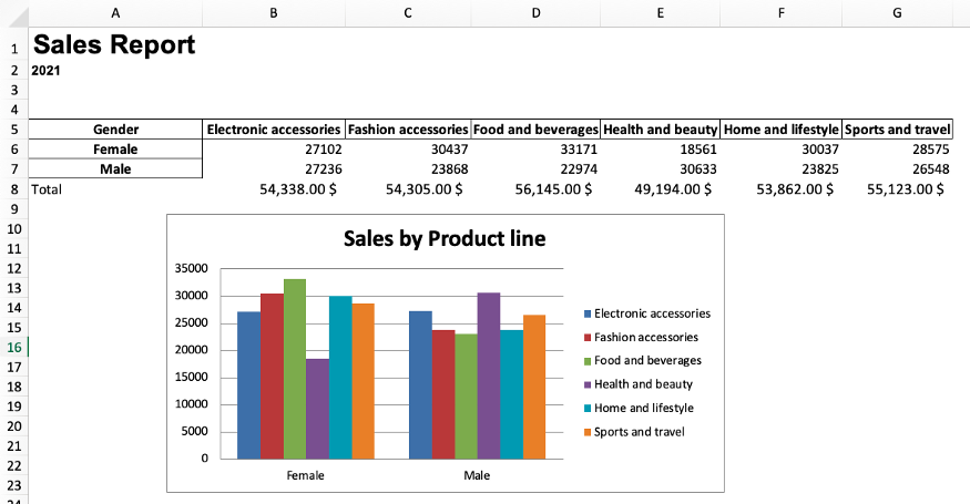
Теперь давайте сделаем этот отчет и автоматизируем его составление с помощью Python!

Создание сводной таблицы с помощью pandas

Импорт библиотек

Теперь, когда вы скачали файл Excel, давайте импортируем библиотеки, которые нам понадобятся.

import pandas as pd
import openpyxl
from openpyxl import load_workbook
from openpyxl.styles import Font
from openpyxl.chart import BarChart, Reference
import string

Чтобы прочитать файл Excel, создать сводную таблицу и экспортировать ее в Excel, мы будем использовать Pandas. Затем мы воспользуемся библиотекой openpyxl для написания формул Excel, создания диаграмм и форматирования электронной таблицы с помощью Python. Наконец, мы создадим функцию на Python для автоматизации всего этого процесса.

Примечание. Если у вас не установлены эти библиотеки в Python, вы можете легко установить их, выполнив pip install pandas и pip install openpyxl в командной строке.

[python_ad_block]

Чтение файла Excel

Прежде чем читать Excel-файл, убедитесь, что он находится там же, где и ваш файл со скриптом на Python. Затем можно прочитать файл Excel с помощью pd.read_excel(), как показано в следующем коде:

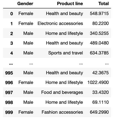
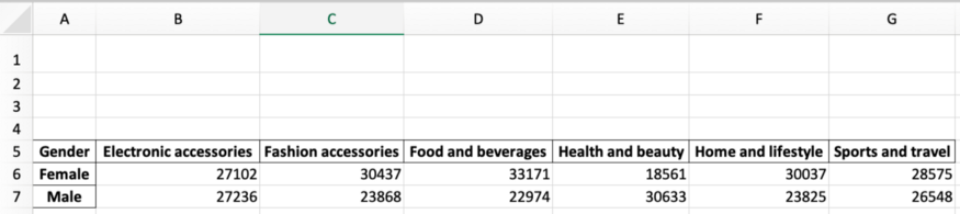
excel_file = pd.read_excel('supermarket_sales.xlsx')
excel_file[['Gender', 'Product line', 'Total']]

В файле много столбцов, но для нашего отчета мы будем использовать только столбцы Gender, Product line и Total. Чтобы показать вам, как они выглядят, я выбрал их с помощью двойных скобок. Если мы выведем это в Jupyter Notebooks, увидим следующий фрейм данных, похожий на таблицу Excel:

Создание сводной таблицы

Теперь мы можем легко создать сводную таблицу из ранее созданного фрейма данных excel_file. Для этого нам просто нужно использовать метод .pivot_table().

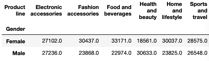
Предположим, мы хотим создать сводную таблицу, которая показывает, сколько в целом потратили на разные продуктовые линейки мужчины и женщины. Для этого мы пишем следующий код:

report_table = excel_file.pivot_table(index='Gender',
                                      columns='Product line',
                                      values='Total',
                                      aggfunc='sum').round(0)

Таблица report_table должна выглядеть примерно так:

Экспорт сводной таблицы в файл Excel

Чтобы экспортировать созданную сводную таблицу, мы используем метод .to_excel(). Внутри скобок нужно написать имя выходного файла Excel. В данном случае давайте назовем этот файл report_2021.xlsx.

Мы также можем указать имя листа, который хотим создать, и в какой ячейке должна находиться сводная таблица.

report_table.to_excel('report_2021.xlsx',
                      sheet_name='Report',
                      startrow=4)

Теперь файл Excel экспортируется в ту же папку, в которой находится ваш скрипт Python.

Создание отчета с помощью openpyxl

Каждый раз, когда мы захотим получить доступ к файлу, мы будем использовать load_workbook(), импортированный из openpyxl. В конце работы мы будем сохранять полученные результаты с помощью метода .save().

В следующих разделах мы будем загружать и сохранять файл при каждом изменении. Вам это нужно сделать только один раз (как в полном коде, показанном в самом конце этого руководства).

Создание ссылки на строку и столбец

Чтобы автоматизировать отчет, нам нужно взять минимальный и максимальный активный столбец или строку, чтобы код, который мы собираемся написать, продолжал работать, даже если мы добавим больше данных.

Чтобы получить ссылки в книге Excel, мы сначала загружаем её с помощью функции load_workbook() и находим лист, с которым хотим работать, используя wb[‘имя листа’]. Затем мы получаем доступ к активным ячейкам с помощью метода .active.

wb = load_workbook('report_2021.xlsx')
sheet = wb['Report']
# cell references (original spreadsheet) 
min_column = wb.active.min_column
max_column = wb.active.max_column
min_row = wb.active.min_row
max_row = wb.active.max_row

Давайте выведем на экран созданные нами переменные, чтобы понять, что они означают. В данном случае мы получим следующие числа:

Min Columns: 1
Max Columns: 7
Min Rows: 5
Max Rows: 7

Откройте файл report_2021.xlsx, который мы экспортировали ранее, чтобы убедиться в этом.

Как видно на картинке, минимальная строка – 5, максимальная — 7. Кроме того, минимальная ячейка – это A1, а максимальная – G7. Эти ссылки будут чрезвычайно полезны для следующих разделов.

Добавление диаграмм в Excel при помощи Python

Чтобы создать диаграмму в Excel на основе созданной нами сводной таблицы, нужно использовать модуль Barchart. Его мы импортировали ранее. Для определения позиций значений данных и категорий мы используем модуль Reference из openpyxl (его мы тоже импортировали в самом начале).

wb = load_workbook('report_2021.xlsx')
sheet = wb['Report']
# barchart
barchart = BarChart()
#locate data and categories
data = Reference(sheet,
                 min_col=min_column+1,
                 max_col=max_column,
                 min_row=min_row,
                 max_row=max_row) #including headers
categories = Reference(sheet,
                       min_col=min_column,
                       max_col=min_column,
                       min_row=min_row+1,
                       max_row=max_row) #not including headers
# adding data and categories
barchart.add_data(data, titles_from_data=True)
barchart.set_categories(categories)
#location chart
sheet.add_chart(barchart, "B12")
barchart.title = 'Sales by Product line'
barchart.style = 5 #choose the chart style
wb.save('report_2021.xlsx')

После написания этого кода файл report_2021.xlsx должен выглядеть следующим образом:

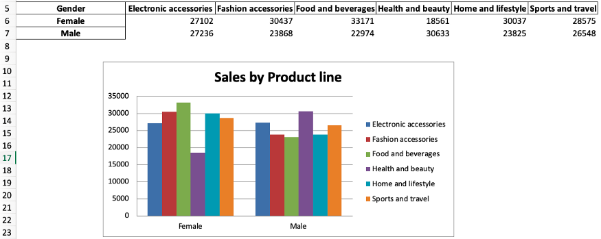
Объяснение кода:

barchart = BarChart() инициализирует переменную barchart из класса Barchart.
data и categories – это переменные, которые показывают, где находится необходимая информация. Для автоматизации мы используем ссылки на столбцы и строки, которые определили выше. Также имейте в виду, что мы включаем заголовки в данные, но не в категории.
Мы используем add_data() и set_categories(), чтобы добавить необходимые данные в гистограмму. Внутри add_data() добавим title_from_data = True, потому что мы включили заголовки для данных.
Метод sheet.add_chart() используется для указания, что мы хотим добавить нашу гистограмму в лист Report. Также мы указываем, в какую ячейку мы хотим её добавить.
Дальше мы изменяем заголовок и стиль диаграммы, используя barchart.title и barchart.style.
И наконец, сохраняем все изменения с помощью wb.save()

Вот и всё! С помощью данного кода мы построили диаграмму в Excel.

Вы можете набирать формулы в Excel при помощи Python так же, как вы это делаете непосредственно на листе Excel.

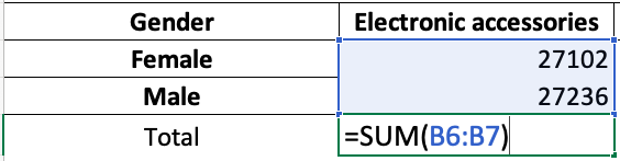
Предположим, мы хотим суммировать данные в ячейках B5 и B6 и отображать их в ячейке B7. Кроме того, мы хотим установить формат ячейки B7 как денежный. Сделать мы это можем следующим образом:

sheet['B7'] = '=SUM(B5:B6)'
sheet['B7'].style = 'Currency'

Довольно просто, не правда ли? Мы можем протянуть эту формулу от столбца B до G или использовать цикл for для автоматизации. Однако сначала нам нужно получить алфавит, чтобы ссылаться на столбцы в Excel (A, B, C, …). Для этого воспользуемся библиотекой строк и напишем следующий код:

import string
alphabet = list(string.ascii_uppercase)
excel_alphabet = alphabet[0:max_column] 
print(excel_alphabet)

Если мы распечатаем excel_alphabet, мы получим список от A до G.

Так происходит потому, что сначала мы создали алфавитный список от A до Z, а затем взяли срез [0:max_column], чтобы сопоставить длину этого списка с первыми 7 буквами алфавита (A-G).

Примечание. Нумерация в Python начинаются с 0, поэтому A = 0, B = 1, C = 2 и так далее. Срез [a:b] возвращает элементы от a до b-1.

Применение формулы к нескольким ячейкам

После этого пройдемся циклом по столбцам и применим формулу суммы, но теперь со ссылками на столбцы. Таким образом вместо того, чтобы многократно писать это:

sheet['B7'] = '=SUM(B5:B6)'
sheet['B7'].style = 'Currency'

мы используем ссылки на столбцы и помещаем их в цикл for:

wb = load_workbook('report_2021.xlsx')
sheet = wb['Report']
# sum in columns B-G
for i in excel_alphabet:
    if i!='A':
        sheet[f'{i}{max_row+1}'] = f'=SUM({i}{min_row+1}:{i}{max_row})'
        sheet[f'{i}{max_row+1}'].style = 'Currency'
# adding total label
sheet[f'{excel_alphabet[0]}{max_row+1}'] = 'Total'
wb.save('report_2021.xlsx')

После запуска кода мы получаем формулу суммы в строке Total для столбцов от B до G:

Посмотрим, что делает данный код:

for i in excel_alphabet проходит по всем активным столбцам, кроме столбца A (if i! = 'A'), так как столбец A не содержит числовых данных
запись sheet[f'{i}{max_row+1}'] = f'=SUM({i}{min_row+1}:{i}{max_row}' это то же самое, что и sheet['B7'] = '=SUM(B5:B6)', только для столбцов от A до G
строчка sheet [f '{i} {max_row + 1}'].style = 'Currency' задает денежный формат ячейкам с числовыми данными (т.е. тут мы опять же исключаем столбец А)
мы добавляем запись Total в столбец А под максимальной строкой (т.е. под седьмой), используя код [f '{excel_alphabet [0]} {max_row + 1}'] = 'Total'

Форматирование листа с отчетом

Теперь давайте внесем финальные штрихи в наш отчет. Мы можем добавить заголовок, подзаголовок, а также настроить их шрифт.

wb = load_workbook('report_2021.xlsx')
sheet = wb['Report']
sheet['A1'] = 'Sales Report'
sheet['A2'] = '2021'
sheet['A1'].font = Font('Arial', bold=True, size=20)
sheet['A2'].font = Font('Arial', bold=True, size=10)
wb.save('report_2021.xlsx')

Вы также можете добавить другие параметры внутри Font(). В документации openpyxl можно найти список доступных стилей.

Итоговый отчет должен выглядеть следующим образом:

Автоматизация отчета с помощью функции Python

Теперь, когда отчет готов, мы можем поместить весь наш код в функцию, которая автоматизирует создание отчета. И в следующий раз, когда мы захотим создать такой отчет, нам нужно будет только ввести имя файла и запустить код.

Примечание. Чтобы эта функция работала, имя файла должно иметь структуру «sales_month.xlsx». Кроме того, мы добавили несколько строк кода, которые используют месяц/год файла продаж в качестве переменной, чтобы мы могли повторно использовать это в итоговом файле и подзаголовке отчета.

Приведенный ниже код может показаться устрашающим, но это просто объединение всего того, что мы написали выше. Плюс новые переменные file_name, month_name и month_and_extension.

import pandas as pd
import openpyxl
from openpyxl import load_workbook
from openpyxl.styles import Font
from openpyxl.chart import BarChart, Reference
import string

def automate_excel(file_name):
    """The file name should have the following structure: sales_month.xlsx"""
    # read excel file
    excel_file = pd.read_excel(file_name)
    # make pivot table
    report_table = excel_file.pivot_table(index='Gender', columns='Product line', values='Total', aggfunc='sum').round(0)
    # splitting the month and extension from the file name
    month_and_extension = file_name.split('_')[1]
    # send the report table to excel file
    report_table.to_excel(f'report_{month_and_extension}', sheet_name='Report', startrow=4)
    # loading workbook and selecting sheet
    wb = load_workbook(f'report_{month_and_extension}')
    sheet = wb['Report']
    # cell references (original spreadsheet)
    min_column = wb.active.min_column
    max_column = wb.active.max_column
    min_row = wb.active.min_row
    max_row = wb.active.max_row
    # adding a chart
    barchart = BarChart()
    data = Reference(sheet, min_col=min_column+1, max_col=max_column, min_row=min_row, max_row=max_row) #including headers
    categories = Reference(sheet, min_col=min_column, max_col=min_column, min_row=min_row+1, max_row=max_row) #not including headers
    barchart.add_data(data, titles_from_data=True)
    barchart.set_categories(categories)
    sheet.add_chart(barchart, "B12") #location chart
    barchart.title = 'Sales by Product line'
    barchart.style = 2 #choose the chart style
    # applying formulas
    # first create alphabet list as references for cells
    alphabet = list(string.ascii_uppercase)
    excel_alphabet = alphabet[0:max_column] #note: Python lists start on 0 -> A=0, B=1, C=2. #note2 the [a:b] takes b-a elements
    # sum in columns B-G
    for i in excel_alphabet:
        if i!='A':
            sheet[f'{i}{max_row+1}'] = f'=SUM({i}{min_row+1}:{i}{max_row})'
            sheet[f'{i}{max_row+1}'].style = 'Currency'
    sheet[f'{excel_alphabet[0]}{max_row+1}'] = 'Total'
    # getting month name
    month_name = month_and_extension.split('.')[0]
    # formatting the report
    sheet['A1'] = 'Sales Report'
    sheet['A2'] = month_name.title()
    sheet['A1'].font = Font('Arial', bold=True, size=20)
    sheet['A2'].font = Font('Arial', bold=True, size=10)
    wb.save(f'report_{month_and_extension}')
    return

Применение функции к одному файлу Excel

Представим, что исходный файл, который мы загрузили, имеет имя sales_2021.xlsx вместо supermarket_sales.xlsx. Чтобы применить формулу к отчету, пишем следующее:

automate_excel('sales_2021.xlsx')

После запуска этого кода вы получите файл Excel с именем report_2021.xlsx в той же папке, где находится ваш скрипт Python.

Применение функции к нескольким файлам Excel

Представим, что теперь у нас есть только ежемесячные файлы Excel sales_january.xlsx, sales_february.xlsx и sales_march.xlsx (эти файлы можно найти на GitHub).

Вы можете применить нашу функцию к ним всем, чтобы получить 3 отчета.

automate_excel('sales_january.xlsx')
automate_excel('sales_february.xlsx')
automate_excel('sales_march.xlsx')

Или можно сначала объединить эти три отчета с помощью pd.concat(), а затем применить функцию только один раз.

# read excel files
excel_file_1 = pd.read_excel('sales_january.xlsx')
excel_file_2 = pd.read_excel('sales_february.xlsx')
excel_file_3 = pd.read_excel('sales_march.xlsx')
# concatenate files
new_file = pd.concat([excel_file_1,
                      excel_file_2,
                      excel_file_3], ignore_index=True)
# export file
new_file.to_excel('sales_2021.xlsx')
# apply function
automate_excel('sales_2021.xlsx')

Заключение

Код на Python, который мы написали в этом руководстве, можно запускать на вашем компьютере по расписанию. Для этого нужно просто использовать планировщик задач или crontab. Вот и все!

В этой статье мы рассмотрели, как автоматизировать создание базового отчета в Excel. В дальнейшем вы сможете создавать и более сложные отчеты. Надеемся, это упростит вашу жизнь. Успехов в написании кода!

Перевод статьи «A Simple Guide to Automate Your Excel Reporting with Python».

Источник

Improve Article

Save Article

Like Article

Read

Discuss

Improve Article

Save Article

Like Article

Prerequisite: Reading & Writing to excel sheet using openpyxl Openpyxl is a Python library using which one can perform multiple operations on excel files like reading, writing, arithmetic operations and plotting graphs. Let’s see how to plot different charts using realtime data. Charts are composed of at least one series of one or more data points. Series themselves are comprised of references to cell ranges. For plotting the charts on an excel sheet, firstly, create chart object of specific chart class( i.e BarChart, LineChart etc.). After creating chart objects, insert data in it and lastly, add that chart object in the sheet object.

Code #1 : Plot the Bar Chart For plotting the bar chart on an excel sheet, use BarChart class from openpyxl.chart submodule.

Python3

import openpyxl

from openpyxl.chart import BarChart,Reference

wb = openpyxl.Workbook()

sheet = wb.active

for i in range(10):

sheet.append([i])

values = Reference(sheet, min_col = 1, min_row = 1,

max_col = 1, max_row = 10)

chart = BarChart()

chart.add_data(values)

chart.title = " BAR-CHART "

chart.x_axis.title = " X_AXIS "

chart.y_axis.title = " Y_AXIS "

sheet.add_chart(chart, "E2")

wb.save("barChart.xlsx")

Output: 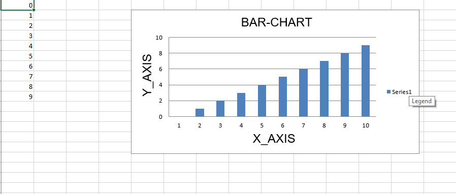Code #2 : Plot the 3D Bar Chart For plotting the 3D bar chart on an excel sheet, use BarChart3D class from openpyxl.chart submodule.

Python3

import openpyxl

from openpyxl.chart import BarChart3D,Reference

for i in range(10):

sheet.append([i])

values = Reference(sheet, min_col = 1, min_row = 1,

max_col = 1, max_row = 10)

chart = BarChart3D()

chart.add_data(values)

chart.title = " BAR-CHART3D "

chart.x_axis.title = " X AXIS "

chart.y_axis.title = " Y AXIS "

sheet.add_chart(chart, "E2")

wb.save("BarChart3D.xlsx")

Output: 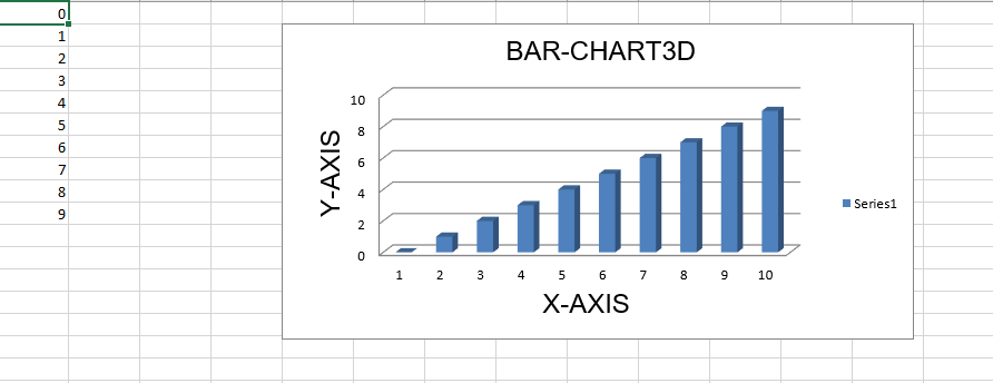Code #3 : Plot the Area Chart For plotting the Area chart on an excel sheet, use AreaChart class from openpyxl.chart submodule.

Python3

import openpyxl

from openpyxl.chart import AreaChart,Reference

wb = openpyxl.Workbook()

sheet = wb.active

for i in range(10):

sheet.append([i])

values = Reference(sheet, min_col = 1, min_row = 1,

max_col = 1, max_row = 10)

chart = AreaChart()

chart.add_data(values)

chart.title = " AREA-CHART "

chart.x_axis.title = " X-AXIS "

chart.y_axis.title = " Y-AXIS "

sheet.add_chart(chart, "E2")

wb.save("AreaChart.xlsx")

Output: 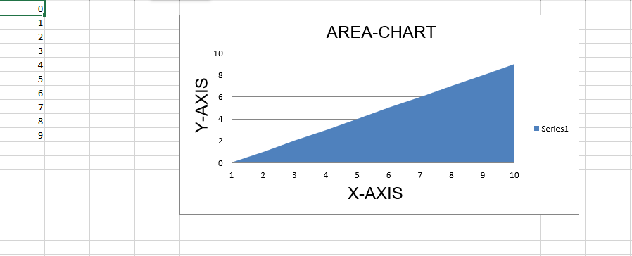Code #4 : Plot the 3D Area Chart For plotting the 3D Area chart on an excel sheet, use AreaChart3D class from openpyxl.chart submodule.

Python3

import openpyxl

from openpyxl.chart import AreaChart3D,Reference

wb = openpyxl.Workbook()

sheet = wb.active

for i in range(10):

sheet.append([i])

values = Reference(sheet, min_col = 1, min_row = 1,

max_col = 1, max_row = 10)

chart = AreaChart3D()

chart.add_data(values)

chart.title = " AREA-CHART3D "

chart.x_axis.title = " X-AXIS "

chart.y_axis.title = " Y-AXIS "

sheet.add_chart(chart, "E2")

wb.save("AreaChart3D.xlsx")

Output: 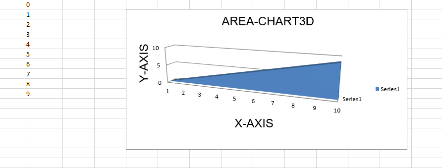Code #5 : Plot a Line Chart. For plotting the Line chart on an excel sheet, use LineChart class from openpyxl.chart submodule.

Python3

import openpyxl

from openpyxl.chart import LineChart,Reference

wb = openpyxl.Workbook()

sheet = wb.active

for i in range(10):

sheet.append([i])

values = Reference(sheet, min_col = 1, min_row = 1,

max_col = 1, max_row = 10)

chart = LineChart()

chart.add_data(values)

chart.title = " LINE-CHART "

chart.x_axis.title = " X-AXIS "

chart.y_axis.title = " Y-AXIS "

sheet.add_chart(chart, "E2")

wb.save("LineChart.xlsx")

Output: 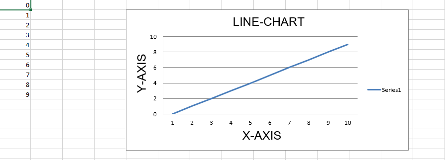Code #6 : Plot a 3D Line Chart. For plotting the 3D Line chart on an excel sheet we have to use LineChart3D class from openpyxl.chart submodule.

Python3

import openpyxl

from openpyxl.chart import LineChart3D,Reference

wb = openpyxl.Workbook()

sheet = wb.active

for i in range(10):

sheet.append([i])

values = Reference(sheet, min_col = 1, min_row = 1,

max_col = 1, max_row = 10)

chart = LineChart3D()

chart.add_data(values)

chart.title = " LINE-CHART3D "

chart.x_axis.title = " X-AXIS "

chart.y_axis.title = " Y-AXIS "

sheet.add_chart(chart, "E2")

wb.save("LineChart3D.xlsx")

Output: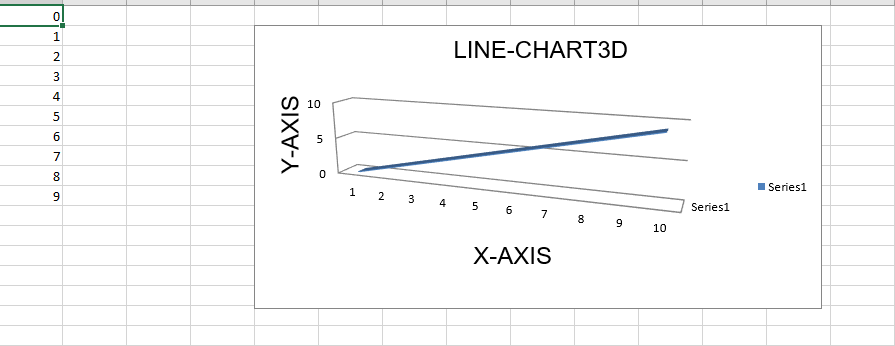

Like Article

Save Article

Источник