
Содержание
- Paste options
- Verify and fix cell references in a pasted formula
- Need more help?
- Copy and paste specific cell contents
- Paste menu options
- Paste Special options
- Paste options
- Operation options
- Other options
Paste options
By default when you copy (or cut) and paste in Excel, everything in the source cell or range—data, formatting, formulas, validation, comments—is pasted to the destination cell(s). This is what happens when you press CTRL+V to paste. Since that might not be what you want, you have many other paste options, depending on what you copy.
For example, you might want to paste the contents of a cell, but not its formatting. Or maybe you want to transpose the pasted data from rows to columns. Or, you might need to paste the result of a formula instead of the formula itself.
Important: When you copy and paste formulas, you might need to fix cell references. However, references are not changed when you cut and paste formulas.
Paste menu options (on the ribbon)
Select Home, select the clipboard icon ( Paste) and pick the specific paste option you want. For example, to paste only formatting from the copied cell, select Formatting  . This table shows the options available in the Paste menu:

All cell contents.

Keep Source Column Widths
Copied cell content along with its column width.

Reorients the content of copied cells when pasting. Data in rows is pasted into columns and vice versa.

Formula(s), without formatting or comments.

Formula results, without formatting or comments.
Only the formatting from the copied cells.

Values & Source Formatting
Values and formatting from copied cells.

Reference to the source cells instead of the copied cell contents.


Copied image with a link to the original cells (if you make any changes to the original cells those changes are reflected in the pasted image).
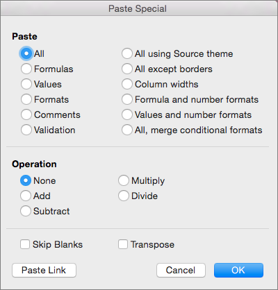
To use options from the Paste Special box, select Home, select the clipboard icon ( Paste), and select Paste Special.
Keyboard Shortcut: Press Ctrl+Alt+V.
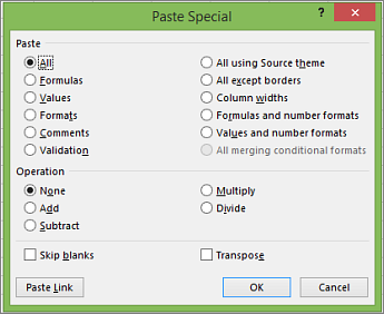
In the Paste Special box, pick the attribute you want to paste.
Note: Depending on the type of data you copied and the Paste option you picked, some other options might be grayed out.
Pastes all cell contents and formatting of the copied data.
Pastes only the formulas of the copied data as entered in the formula bar.
Pastes only the values of the copied data as displayed in the cells.
Pastes only cell formatting of the copied data.
Comments and Notes
Pastes only comments and notes attached to the copied cell.
Pastes data validation rules for the copied cells to the paste area.
All using Source theme
Pastes all cell contents in the document theme formatting that is applied to the copied data.
All except borders
Pastes all cell contents and formatting applied to the copied cell except borders.
Pastes the width of one copied column or range of columns to another column or range of columns.
Formulas and number formats
Pastes only formulas and all number formatting options from the copied cells.
Values and number formats
Pastes only values and all number formatting options from the copied cells.
All merging conditional formats
Pastes the contents and conditional formatting options from the copied cells.
You can also specify a mathematical operation to apply to the copied data.
Specifies that no mathematical operation will be applied to the copied data.
Adds the copied data to the data in the destination cell or range of cells.
Subtracts the copied data from the data in the destination cell or range of cells.
Multiplies the copied data with the data in the destination cell or range of cells.
Divides the copied data by the data in the destination cell or range of cells.
Avoids replacing values in your paste area when blank cells occur in the copy area when you select this check box.
Changes columns of copied data to rows and vice versa when you select this check box.
Click to create a link to the copied cell(s).
Verify and fix cell references in a pasted formula
Note: Cell references are automatically adjusted when you cut (not copy) and paste formulas.
After you paste a copied formula, you should verify that all cell references are correct in the new location. The cell references may have changed based on the reference type (absolute, relative, or mixed) used in the formula.
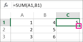
For example, if you copy a formula in cell A1 and paste it two cells down and to the right (C3), cell references in the pasted formula will change as follows:
$A$1 (absolute column and absolute row)
A$1 (relative column and absolute row)
$A1 (absolute column and relative row)
A1 (relative column and relative row)
If cell references in the formula don’t give you the result you want, try switching to different reference types:
Select the cell containing the formula.
In the formula bar  , select the reference you want to change.
Press F4 to switch between the reference combinations, and choose the one you want.
For more information about cell references, see Overview of formulas.
When you copy in Excel for the web, you can pick paste options in the destination cells.
Select Home, select the clipboard icon, select Paste, and pick the specific paste option you want. For example, to paste only formatting from the copied cell, select Paste Formatting . This table shows the options available in the Paste menu:
All cell contents.
Formula(s), without formatting.
Formula results, without formatting.
Only the formatting from the copied cells.
All cell content, but reorients the content when pasting. Data in rows is pasted into columns and vice versa.
Need more help?
You can always ask an expert in the Excel Tech Community or get support in the Answers community.
Источник
Copy and paste specific cell contents
You can copy and paste specific cell contents or attributes (such as formulas, formats, comments, and validation). By default, if you use the Copy  and Paste
  icons (or
  + C and + V), all attributes are copied. To pick a specific paste option, you can either use a Paste menu option or select Paste Special, and pick an option from the Paste Special box. Attributes other than what you select are excluded when you paste.

Select the cells that contain the data or other attributes that you want to copy.
On the Home tab, click Copy .
Click the first cell in the area where you want to paste what you copied.
On the Home tab, click the arrow next to Paste, and then do any of the following. The options on the Paste menu will depend on the type of data in the selected cells:
All cell contents and formatting, including linked data.
Only the formulas.
Formulas & Number Formatting
Only formulas and number formatting options.
Keep Source Formatting
All cell contents and formatting.
All cell contents and formatting except cell borders.
Keep Source Column Widths
Only column widths.
Reorients the content of copied cells when pasting. Data in rows is pasted into columns and vice versa.
Only the values as displayed in the cells.
Values & Number Formatting
Only the values and number formatting.
Values & Source Formatting
Only the values and number color and font size formatting.
All cell formatting, including number and source formatting.
Link the pasted data to the original data. When you paste a link to the data that you copied, Excel enters an absolute reference to the copied cell or range of cells in the new location.
Paste as Picture
A copy of the image.
A copy of the image with a link to the original cells (if you make any changes to the original cells those changes are reflected in the pasted image).
Paste the width of one column or range of columns to another column or range of columns.
Merge conditional formatting
Combine conditional formatting from the copied cells with conditional formatting present in the paste area.
Paste Special options
Select the cells that contain the data or other attributes that you want to copy.
On the Home tab, click Copy .
Click the first cell in the area where you want to paste what you copied.
On the Home tab, click the arrow next to Paste, and then select Paste Special.
Select the options you want.
Paste options
All cell contents and formatting, including linked data.
Only the formulas.
Only the values as displayed in the cells.
Cell contents and formatting.
Only comments attached to the cell.
Only data validation rules.
All using Source theme
All cell contents and formatting using the theme that was applied to the source data.
All except borders
Cell contents and formatting except cell borders.
The width of one column or range of columns to another column or range of columns.
Formulas and number formats
Only formulas and number formatting.
Values and number formats
Only values and number formatting options from the selected cells.
All, merge conditional formats
Combine conditional formatting from the copied cells with conditional formatting present in the paste area.
Operation options
The Operation options mathematically combine values between the copy and paste areas.
Paste the contents of the copy area without a mathematical operation.
Add the values in the copy area to the values in the paste area.
Subtract the values in the copy area from the values in the paste area.
Multiply the values in the paste area by the values in the copy area.
Divide the values in the paste area by the values in the copy area.
Other options
Avoid replacing values or attributes in your paste area when blank cells occur in the copy area.
Reorients the content of copied cells when pasting. Data in rows is pasted into columns and vice versa.
If data is a picture, links to the source picture. If the source picture is changed, this one will change too.
Tip: Some options are available both on the Paste menu and in the Paste Special dialog box. The option names might vary a bit but the results are the same.
Select the cells that contain the data or other attributes that you want to copy.
On the Standard toolbar, click Copy  .
.
Click the first cell in the area where you want to paste what you copied.
On the Home tab, under Edit, click Paste, and then click Paste Special.
On the Paste Special dialog, under Paste, do any of the following:
Paste all cell contents and formatting, including linked data.
Paste only the formulas as entered in the formula bar.
Paste only the values as displayed in the cells.
Paste only cell formatting.
Paste only comments attached to the cell.
Paste data validation rules for the copied cells to the paste area.
All using Source theme
Paste all cell contents and formatting using the theme that was applied to the source data.
All except borders
Paste all cell contents and formatting except cell borders.
Paste the width of one column or range of columns to another column or range of columns.
Formulas and number formats
Paste only formulas and number formatting options from the selected cells.
Values and number formats
Paste only values and number formatting options from the selected cells.
Merge conditional formatting
Combine conditional formatting from the copied cells with conditional formatting present in the paste area.
To mathematically combine values between the copy and paste areas, in the Paste Special dialog box, under Operation, click the mathematical operation that you want to apply to the data that you copied.
Paste the contents of the copy area without a mathematical operation.
Add the values in the copy area to the values in the paste area.
Subtract the values in the copy area from the values in the paste area.
Multiply the values in the paste area by the values in the copy area.
Divide the values in the paste area by the values in the copy area.
Additional options determine how blank cells are handled when pasted, whether copied data is pasted as rows or columns, and linking the pasted data to the copied data.
Avoid replacing values in your paste area when blank cells occur in the copy area.
Change columns of copied data to rows, or vice versa.
Link the pasted data to the original data. When you paste a link to the data that you copied, Excel enters an absolute reference to the copied cell or range of cells in the new location.
Note: This option is available only when you select All or All except borders under Paste in the Paste Special dialog box
Tip: In Excel for Mac version 16.33 or higher, the «paste formatting», «paste formulas», and «paste values» actions can be added to your quick-access toolbar (QAT) or assigned to custom key combinations. For the keyboard shortcuts, you’ll need to assign a key combination that isn’t already being used to open the Paste Special dialog.
Источник
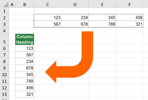
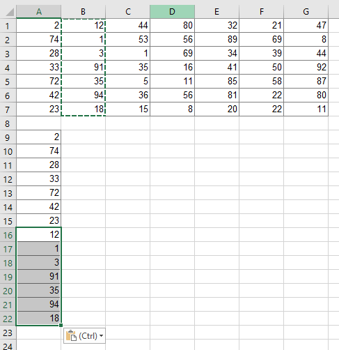
Say, you have an Excel table and want to copy all column underneath each other so that you only have one column. For example, you have a table 2 rows by 4 columns like in the screenshot on the right-hand side. You want to copy and paste this table to one column. You often need such transformation for inserting PivotTables or to create database formats. This article provides 4 simple methods to transform a 2-dimensional table into one column in Excel.
Example
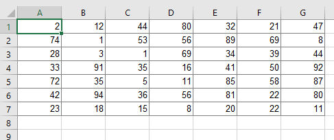
The following methods will be introduced with a simplified example as shown on the right-hand side. You have a table with numbers within the cell range A1 to G7. That means you have 7 rows and also 7 columns. In total 49 cells to be copied to one column.
Method 1: Copy table to one column manually
Like so often, copying and pasting the columns manually might be the fastest solution. Given that you are reading this article, this might not be the method you want to hear. But anyway, doing it manually is often the fastest way.
Maybe some advice to speed up the manual process might help. Try to use as many keyboard shortcuts as possible. That way you could save some time.
- Holding Ctrl and pressing one of the arrow keys makes you jump between tables and cells.
- Holding the Shift key, you can select cells and ranges.
- And – of course – with Ctrl + C and Ctrl + V you can copy and paste cells.
For more information about the keyboard shortcuts please refer to our big keyboard shortcut package.
Method 2: The INDEX formula
You can convert a two-dimensional table into just one column by using the INDEX formula. Unfortunately, it requires some preparations. But on the other hand, it’s one of the faster ways (compared to setting up the more complex OFFSET formula like in method 3 below or the INDIRECT formula).
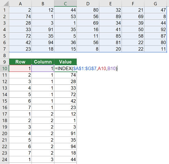
Let’s see what you need to prepare. Basically you have to create the column and row number in additional helper columns. That way you can easily refer to the original table. The screenshot on the right-hand side shows the necessary preparations.
- You need one column containing the row number (here in column A). You always start with 1. So if you data start in row 3, the first number you write is still 1.
- You need one column containing the column number (here in column B). Also for the column number you always start with number one.
- The third column contains the actual values, pulled by the formula =INDEX($A$1:$G$7;A10;B10) . Example: In cell C10, the INDEX formula returns the value from the first row and first column of the range A1 to G7.
Please refer to this article for more information about the INDEX formula in Excel.
Method 3: OFFSET formula
The third method uses the OFFSET formula for copying several columns underneath each other to one column. If you need some introduction to the OFFSET formula, please refer to this article.
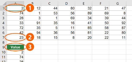
Because the formula is – in this universal case – very long, we don’t go much into detail here. It’s based on three cells.
- The top left cell of the table you want to convert (here: A1).
- The bottom left cell of the table you want to convert (here: A7).
- The heading cell of your single column, which is supposed to contain all the data from the table (here: A9)
Now you just have to replace the cell links in the following formula with your cells. Don’t forget to fix the references with the $-signs as shown in the formula below.
=OFFSET($A$1,(ROW()-ROW($A$9)-1)-(ROW($A$7)-ROW($A$1)+1)*ROUNDDOWN((ROW()-ROW($A$9)-1)/(ROW($A$7)-ROW($A$1)+1),0),ROUNDDOWN((ROW()-ROW($A$9)-1)/(ROW($A$7)-ROW($A$1)+1),0))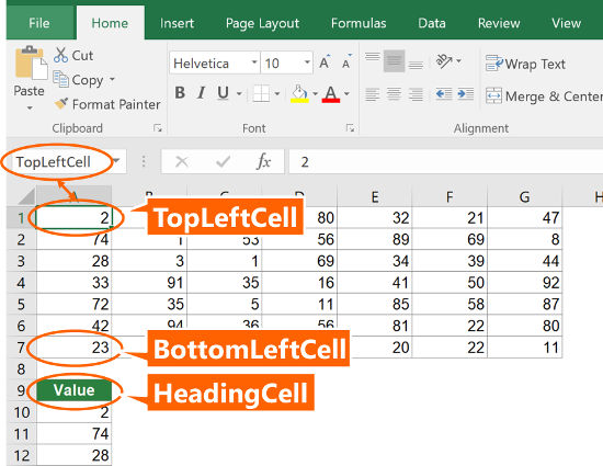
In order to make it easier for you to use the formula, you can use the version below. All you have to do is to give names to the three main cell as shown in the image on the right-hand side. In order to achieve this, select the top left cell of your original table (here: A1) and click into the name field. Type “TopLeftCell” and press Enter on the keyboard. Repeat this with the bottom left cell (name “BottomLeftCell”) as well as the heading cell of your new table (name “HeadingCell”).
Once done, copy and paste the following formula it the first cell (here: A10). Now just copy and paste this cell down until all columns from your original table are covered.
=OFFSET(TopLeftCell,(ROW()-ROW(HeadingCell)-1)-(ROW(BottomLeftCell)-ROW(TopLeftCell)+1)*ROUNDDOWN((ROW()-ROW(HeadingCell)-1)/(ROW(BottomLeftCell)-ROW(TopLeftCell)+1),0),ROUNDDOWN((ROW()-ROW(HeadingCell)-1)/(ROW(BottomLeftCell)-ROW(TopLeftCell)+1),0))Method 4: Professor Excel Tools
You want to use the most convenient way? Try the Excel add-in “Professor Excel Tools”. The steps are shown in the screenshot below.
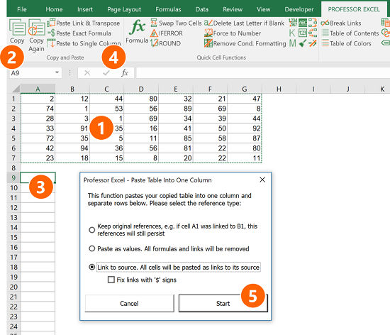
- Select the table you want to transform into a single column.
- Click on Copy on the left-hand side of the “Professor Excel”-ribbon.
- Select the first cell from which Professor Excel should paste the columns underneath.
- Click on “Paste to Single Column” on the “Professor Excel” ribbon.
- Now you can finetune the copy-and-paste-format. Do you which to copy the formulas without changing cell references, do you which to copy them as values or do you want to insert links to the original table? Then press Start.
That’s it. Do you want to try “Professor Excel” for free? Then just follow this link for more information or start the download right away.

This function is included in our Excel Add-In ‘Professor Excel Tools’
(No sign-up, download starts directly)
Download
![]() Please feel free to download all examples shown above in one comprehensive Excel file. Just click on this link and the download starts right away.
Please feel free to download all examples shown above in one comprehensive Excel file. Just click on this link and the download starts right away.
You can use following code. It will paste all values to the column A:
Sub test()
    Dim lastCol As Long, lastRowA As Long, lastRow As Long, i As Long

    'find last non empty column number'
    lastCol = Cells(1, Columns.Count).End(xlToLeft).Column

    'loop through all columns, starting from column B'
    For i = 2 To lastCol
        'find last non empty row number in column A'
        lastRowA = Cells(Rows.Count, "A").End(xlUp).Row
        'find last non empty row number in another column'
        lastRow = Cells(Rows.Count, i).End(xlUp).Row

        'copy data from another column'
        Range(Cells(1, i), Cells(lastRow, i)).Copy
        'paste data to column A'
        Range("A" & lastRowA + 1).PasteSpecial xlPasteValues

        'Clear content from another column. if you don't want to clear content from column, remove next line'
        Range(Cells(1, i), Cells(lastRow, i)).ClearContents
    Next i

    Application.CutCopyMode = False
End Sub
Copying and Pasting a cell or a range of cells is one of the most common tasks users do in Excel.
A proper understanding of how to copy-paste multiple cells (that are adjacent or non-adjacent) would really help you be a lot more efficient while working with Microsoft Excel.
In this tutorial, I will show you different scenarios where you can copy and paste multiple cells in Excel.
If you have been using Excel for some time now, I’m quite sure you would know some of these already, but there’s a good chance you’d end up learning something new.
So let’s get started!
Copy and Paste Multiple Adjacent Cells
Let’s start with the easy scenario.
Suppose you have a range of cells (that are adjacent) as shown below and you want to copy it to some other location in the same worksheet or some other worksheet/workbook.

Below are the steps to do this:
- Select the range of cells that you want to copy

- Right-click on the selection
- Click on Copy

- Right-click on the destination cell (E1 in this example)
- Click on the Paste icon
The above steps would copy all the cells in the selected range and paste them into the destination range.

In case you already have something in the destination range, it would be overwritten.
Excel also gives you the flexibility to choose what you want to paste. For example, you can choose to only copy and paste the values, or the formatting, or the formulas, etc.
These options are available to you when you right-click on the destination cell (the icons below the paste special option).
Or you can click on the Paste Special option and then choose what you want to paste using the options in the dialog box.
Useful Keyboard Shortcuts for Copy Paste
In case you prefer using the keyboard while working with Excel, you can use the below shortcut:
- Control + C (Windows) or Command + C (Mac) – to copy range of cells
- Control + V (Windows) or Command + V (Mac) – to paste in the destination cells
And below are some advanced copy-paste shortcuts (using the paste special dialog box).
To use this, first copy the cells, then select the destination cell, and then use the below keyboard shortcuts.
- To paste only the Values – Control + E + S + V + Enter
- To paste only the Formulas – Control + E + S + F + Enter
- To paste only the Formatting – Control + E + S + T + Enter
- To paste only the Column Width – Control + E + S + W + Enter
- To paste only the Comments and notes – Control + E + S + C + Enter
In case you’re using Mac, use Command instead of Control.
Also read: How to Cut a Cell Value in Excel (Keyboard Shortcuts)
Mouse Shortcut for Copy Paste
If you prefer using the mouse instead of the keyboard shortcuts, here is another way you can quickly copy and paste multiple cells in Excel.
- Select the cells that you want to copy
- Hold the Control key
- Place the mouse cursor at the edge of the selection (you will notice that the cursor changes into an arrow with a plus sign)
- Left-click and then drag the selection where you want the cells to be pasted

This method is also quite fast but is only useful in case you want to copy and paste the range of cells in the same worksheet somewhere nearby.
If the destination cell is a little far off, you’re better off using the keyboard shortcuts.
Copy and Paste Multiple Non-Adjacent Cells
Copy-pasting multiple cells that are nonadjacent is a bit tricky.
If you select multiple cells that are not adjacent to each other, and you copy these cells, you’ll see a prompt as shown below.

This is Excel’s way of telling you that you cannot copy multiple cells that are non-adjacent.
Unfortunately, there’s nothing that you can do about it.
There’s no hack or a workaround, and if you want to copy and paste these nonadjacent cells, you will have to do this one by one.
But there are a few scenarios where you can actually copy and paste non-adjacent cells in Excel.
Let’s have a look at these.
Copy and Paste Multiple Non-Adjacent Cells (that are in the same row/column)
While you can not copy non-adjacent cells in different rows and columns, if you have non-adjacent cells in the same row or column, Excel allows you to copy these.
For example, you can copy cells in the same row (even if these are non-adjacent). Just select the cells and then use Control + C (or Command + C for Mac). You will see the outline (the dancing ants outline).

Once you have copied these cells, go to the destination cell and paste these (Control + V or Command + V)
Excel will paste all the copied cells in the destination cell but make these adjacents.
Similarly, you can select multiple nonadjacent cells in one column, copy them, and then paste it into the destination cells.
Copy and Paste Multiple Non-Adjacent Rows/Columns (but adjacent cells)
Another thing Excel allows is to select non-adjacent rows or non-adjacent columns and then copy them.

Now when you paste these in the destination cell, these would be pasted as adjacent rows or columns.

Below is an example where I copied multiple non-adjacent rows from the dataset and pasted these in a different location.
Copy Value From Above in Non-Adjacent Cells
One practical scenario where you may have to copy and paste multiple cells would be when you have gaps in a data set and you want to copy the value from the cell above.
Below I have some dates in column A, and there are some blank cells as well. I want to fill these blank cells with the date in the last filed cell above them.

To do this, I would need to do two things:
- Select all the blank cells
- Copy the date from the above-filled cell and paste it into these blank cells
Let me show you how to do this.
Select All Blank Cells in the Dataset
Below are the steps to select all the blank cells in column A:
- Select the dates in column A, including the blank ones that you want to fill

- Press the F5 key on your keyboard. This will open the Go To dialog box.
- Click the Special button. This will open the Go To Special dialog box.

- In the Go To Special dialog box, select Blanks

- Click OK
The above steps would select all the blank cells in column A.

Now, we want to somehow copy the value in the above field cell in these blank cells. This cannot be done using any copy-paste method so we will have to use a formula (a very simple one).
Fill Blank Cells with Value Above
This part is really easy.
- With the blank cell selected, first hit the equal to key on your keyboard

- Now hit the Up arrow key. This will automatically enter the cell reference of the cell that is above the active cell.

- Hold the Control key and press the Enter key
The above steps would enter the same formula in all the selected blank cells – which is to refer to the cell above it.

While this is a formula, the end result is that you have the blank cells filled with the above-filled date in the data set.
Once you have the desired result, you can convert the formula into values if you want (so that the formula doesn’t update the cells in case you change any value in a cell that is being referenced in the formula).
So these are a couple of methods you can use to copy and paste multiple cells (adjacent and non-adjacent cells) in Excel. I am sure using these methods will help you save tons of time in your day-to-day work.
I hope you found this tutorial useful!
Other Excel tutorials you may also like:
- How to Copy and Paste Column in Excel? 3 Easy Ways!
- How to Copy Excel Table to MS Word (4 Easy Ways)
- How to Copy Conditional Formatting to Another Cell in Excel
- How to Copy and Paste Formulas in Excel without Changing Cell References
- How to Edit Cells in Excel?
Home / Excel Basics / How to Copy and Paste a Column in Excel
Copying the data is a very frequent task in our day-to-day lives while working in Excel or any other word processing software. Usually, we have to copy a single cell from one place to another or even sometimes in a different worksheet also. It is very easy to do.
But when it comes to copying multiple continuous cells as well as non-adjacent cells then we all find ourselves in very big trouble.
In this tutorial, we will learn methods to copy the single or multiple (continuous, and non-continuous) columns. Now, let’s go through it step-by-step.
- First, select the entire column from its Column Header Letter on the top of it that you want to copy.
- Then, press the right-click button on the mouse and select the “Copy” option from the pop-up box.

- After this, select the range of cells of that particular column where you wish to “Paste” your data.
- Once you are selecting the range, click on the right key of the mouse and choose the paste option from it.


Copying the Column by using a Keyboard Shortcut
Here’s an easier way to copy and paste the data by using the keyboard shortcut instead of doing it manually.
- First of all, click on any cell of the column that you want to copy.
- From here, select the entire column by holding the shortcut key that is (Control + Spacebar).
- Next, you can copy the selected column by pressing the Control + C button on the keyboard.
- Now, you’ll see that column is highlighted, and then paste it by using the Control + V.
Related ➜ Keyboard Shortcuts for Excel (PDF Cheatsheet)
Copy and Paste Multiple Adjacent Columns
If you want to copy multiple columns of the spreadsheet at the same time, you can do this. Here, below are the steps.
- Select the multiple columns in a sequence with the left key of your mouse by the column header.
- Next, right-click on the selected columns.
- Click on the “Copy” option from the dialog box to select the entire data.

- Now, you’ll see that column is highlighted, and then paste it by using the Control + V.


Important Note: Make sure that you have enough blank columns where you would like to paste your data or in case you already have something in that range of cells, then it would be overwritten.
Copy Multiple Non-Adjacent Columns
The simplest way to copy multiple non-adjacent columns is by using the CTRL key. Let’s do it stepwise.
- In your worksheet, select the first column by clicking on its header.
- After that, click on the next columns one by one that you want to highlight by holding down the Control key.
- Following this, right-click on any of the selected columns and choose “Copy” from the dialog box.

- Now, you’ll see all the selected columns have been highlighted on the sheet.
- In the end, select the destination cell where you would like to paste your data and by pressing Control + V you can paste it.


Copy and Paste the column is from the Ribbon
It is an interesting thing to know that you can also copy and paste the values from the ribbon. Let’s do it by the following steps:
- First, select all the columns that you wish to copy.
- Then, go to the Home tab and from the Clipboard> choose Copy or either use (Ctrl + C) from the keyboard to copy the columns.

- Select the particular cell where you wish to paste your data.
- And then, click on the paste from the Ribbon or you can use the shortcut that is (Ctrl + V).


So, these are the ways by which you can copy and paste columns in excel.
Moreover, if you want to copy multiple non-adjacent columns then you can use the third method for this.
Along with this, the above-given shortcut of copy and paste will help you to compile your data as soon as possible.
Paste menu options (on the ribbon)
Select Home, select the clipboard icon (Paste) and pick the specific paste option you want. For example, to paste only formatting from the copied cell, select Formatting . This table shows the options available in the Paste menu:
|
Icon |
Option name |
What is pasted |
|---|---|---|
|
|
Paste |
All cell contents. |
|
|
Keep Source Column Widths |
Copied cell content along with its column width. |
|
|
Transpose |
Reorients the content of copied cells when pasting. Data in rows is pasted into columns and vice versa. |
|
|
Formulas |
Formula(s), without formatting or comments. |
|
|
Values |
Formula results, without formatting or comments. |
|
|
Formatting |
Only the formatting from the copied cells. |
|
|
Values & Source Formatting |
Values and formatting from copied cells. |
|
|
Paste Link |
Reference to the source cells instead of the copied cell contents. |
|
|
Picture |
Copied image. |
|
|
Linked Picture |
Copied image with a link to the original cells (if you make any changes to the original cells those changes are reflected in the pasted image). |
Paste Special
To use options from the Paste Special box, select Home, select the clipboard icon (Paste), and select Paste Special.
Keyboard Shortcut: Press Ctrl+Alt+V.
In the Paste Special box, pick the attribute you want to paste.
Note: Depending on the type of data you copied and the Paste option you picked, some other options might be grayed out.
|
Paste option |
Action |
|
All |
Pastes all cell contents and formatting of the copied data. |
|
Formulas |
Pastes only the formulas of the copied data as entered in the formula bar. |
|
Values |
Pastes only the values of the copied data as displayed in the cells. |
|
Formats |
Pastes only cell formatting of the copied data. |
|
Comments and Notes |
Pastes only comments and notes attached to the copied cell. |
|
Validation |
Pastes data validation rules for the copied cells to the paste area. |
|
All using Source theme |
Pastes all cell contents in the document theme formatting that is applied to the copied data. |
|
All except borders |
Pastes all cell contents and formatting applied to the copied cell except borders. |
|
Column widths |
Pastes the width of one copied column or range of columns to another column or range of columns. |
|
Formulas and number formats |
Pastes only formulas and all number formatting options from the copied cells. |
|
Values and number formats |
Pastes only values and all number formatting options from the copied cells. |
|
All merging conditional formats |
Pastes the contents and conditional formatting options from the copied cells. |
You can also specify a mathematical operation to apply to the copied data.
|
Operation |
Action |
|
None |
Specifies that no mathematical operation will be applied to the copied data. |
|
Add |
Adds the copied data to the data in the destination cell or range of cells. |
|
Subtract |
Subtracts the copied data from the data in the destination cell or range of cells. |
|
Multiply |
Multiplies the copied data with the data in the destination cell or range of cells. |
|
Divide |
Divides the copied data by the data in the destination cell or range of cells. |
|
Other options |
Action |
|---|---|
|
Skip blanks |
Avoids replacing values in your paste area when blank cells occur in the copy area when you select this check box. |
|
Transpose |
Changes columns of copied data to rows and vice versa when you select this check box. |
|
Paste Link |
Click to create a link to the copied cell(s). |
Verify and fix cell references in a pasted formula
Note: Cell references are automatically adjusted when you cut (not copy) and paste formulas.
After you paste a copied formula, you should verify that all cell references are correct in the new location. The cell references may have changed based on the reference type (absolute, relative, or mixed) used in the formula.
For example, if you copy a formula in cell A1 and paste it two cells down and to the right (C3), cell references in the pasted formula will change as follows:
|
This reference: |
Changes to: |
|---|---|
|
$A$1 (absolute column and absolute row) |
$A$1 |
|
A$1 (relative column and absolute row) |
C$1 |
|
$A1 (absolute column and relative row) |
$A3 |
|
A1 (relative column and relative row) |
C3 |
If cell references in the formula don’t give you the result you want, try switching to different reference types:
-
Select the cell containing the formula.
-
In the formula bar
 , select the reference you want to change.
 -
Press F4 to switch between the reference combinations, and choose the one you want.
For more information about cell references, see Overview of formulas.
When you copy in Excel for the web, you can pick paste options in the destination cells.
Select Home, select the clipboard icon, select Paste, and pick the specific paste option you want. For example, to paste only formatting from the copied cell, select Paste Formatting . This table shows the options available in the Paste menu:
|
Icon |
Option name |
What is pasted |
|---|---|---|
|
|
Paste |
All cell contents. |
|
|
Paste Formulas |
Formula(s), without formatting. |
|
|
Paste Values |
Formula results, without formatting. |
|
|
Paste Formatting |
Only the formatting from the copied cells. |
|
|
Paste Transpose |
All cell content, but reorients the content when pasting. Data in rows is pasted into columns and vice versa. |
See all How-To Articles
This tutorial demonstrates how to paste CSV data into columns in Excel and Google Sheets.
Paste CSV Data Into Columns
One way to convert a CSV file to Excel (.xlsx) is to use the Text Import Wizard.
Another option, described below, is to open a CSV file with Notepad, copy and paste all data in one column in Excel, and the use the Text to Columns functionality to split data into columns.
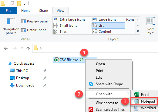
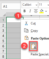
- Navigate to the folder with your CSV file, then (1) right-click the CSV file, (2) click Open with, and (3) choose Notepad.
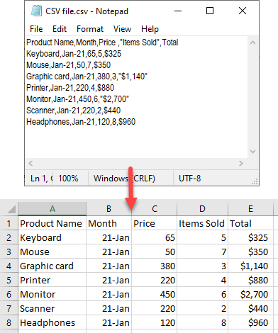
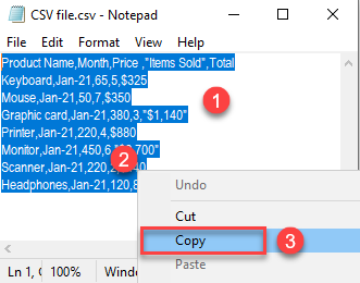
- Data in CSV have comma as a column separator, and every row is in the new line. (1) Select all data in the file (use keyboard shortcut CTRL + A), (2) right-click the selected text, and (3) choose Copy.
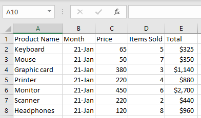
- Now open your Excel file, right-click cell A1, and choose Paste (or use the keyboard shortcut CTRL + V).
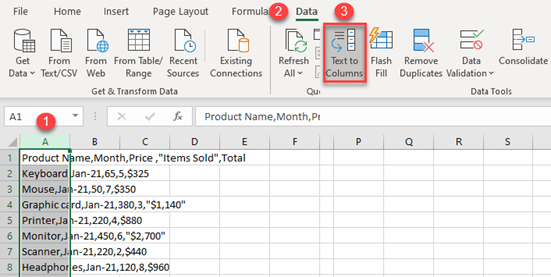
- Select Column A (by clicking on letter A in the column heading), and in the Ribbon, go to Data > Text to Columns.
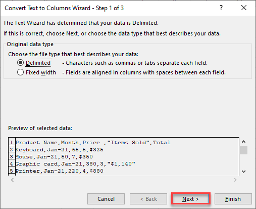
- In the Wizard Step 1, click Next.
- In the Wizard Step 2, choose Comma as delimiter and click Next.
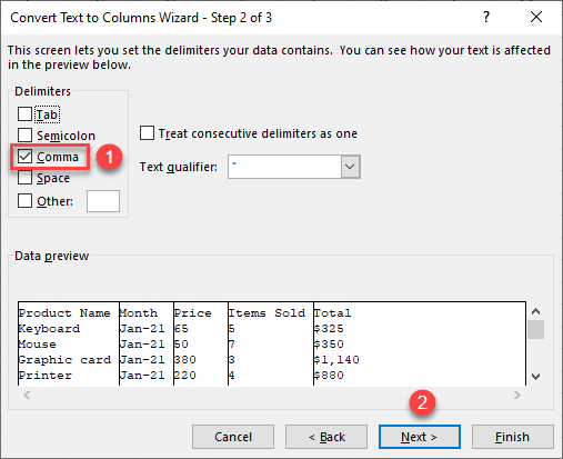
As you can see in the Data preview, values are split into columns based on a comma as a delimiter.
- In the Wizard Step 3, you can format columns as General, Text, or Date. By default, all columns have a General format. Click Finish to complete the wizard.
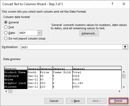
As a result, values from Column A have split into Columns A–E.
Paste CSV Data Into Google Sheets
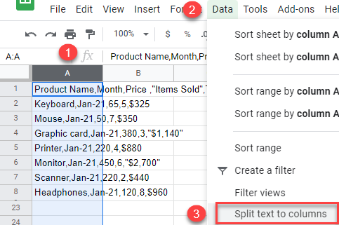
You can also copy and paste CSV data into columns in Google Sheets. First, repeat the first three steps from the previous section to paste data from the text editor to Google Sheets.
Then, select Column A (by clicking on the letter A in the column heading), and in the Menu, go to Data > Split text to columns.
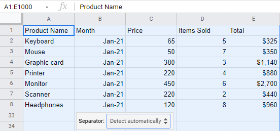
The result is the same as in Excel: All values have split into Columns A–E. In Google Sheets, the separator is automatically detected. In case there is a mistake, you can set it manually in the Separator drop-down list.
Copying and pasting is a very frequently performed action when working on a computer. This is also true in Excel.
It’s so common that almost everyone knows the keyboard shortcuts to copy Ctrl + C and paste Ctrl + V.
When using this in Excel, it will copy everything including values, formulas, formatting, comments/notes, and data validation.
This can be frustrating as sometimes you’ll only want the values to copy and not any of the other stuff in the cells.
In this post, you’ll learn all the ways to copy and paste only the values from your Excel data.
Example Data
The example data used in this post contains various formatting.
- Cell formatting such as font color, fill color, number formatting, and borders.
- Notes.
- SUM formula.
- A data validation dropdown list.
Paste Special Keyboard Shortcut
If you want to copy and paste anything other than an exact copy, then you’re going to need to become familiar with paste special.
A favorite method to use this is with a keyboard shortcut.
To use the paste special keyboard shortcut.
- Copy the data you want to paste as values into your clipboard.
- Choose a new location in your workbook to paste the values into.
- Press Ctrl + Alt + V on your keyboard to open up the Paste Special menu.
- Select Values from the Paste option or press V on your keyboard.
- Press the OK button.
This will paste your data without any formatting, formulas, comments/notes, or data validation. Nothing but the values will be there.
Paste Special Legacy Keyboard Shortcut
This keyboard shortcut is a legacy shortcut from before the Excel ribbon command existed and it’s still usable.
In fact, when you try and use this you’ll be greeted with the above warning to let you know this is from an earlier version of Microsoft Office.
When you have a range of data copied to your clipboard, you can open up the Paste Special menu by pressing Alt + E + S on your keyboard.
Once the Paste Special menu is open you can then press V for Values.
One advantage the legacy shortcut has is it can easily be performed with one hand!
Paste Special Values Keyboard Shortcut
Pasting as values is a very common activity in Excel. Because of this, a new keyboard shortcut was introduced to Microsoft 365 users for this exact purpose.
Press Ctrl + Shift + V on your keyboard to paste the last item in your clipboard as values.
This is the most useful new shortcut as it bypasses the paste special menu entirely.
Paste Special from the Home Tab
If you’re not a keyboard person and prefer using the mouse, then you can access the Paste Values command from the ribbon commands.
Here’s how to use Paste Values from the ribbon.
- Select and copy the data you want to paste into your clipboard.
- Select the cell you want to copy the values into.
- Go to the Home tab.
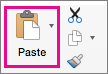
- Click on the lower part of the Paste button in the clipboard section.
- Select the Values clipboard icon from the paste options.
The cool thing about this menu is before you click on any of the commands you will see a preview of the data you’re about to paste. This makes it easy to ensure you’re selecting the right option.
Paste Values with Hotkey Shortcuts
Since the paste values command is in the ribbon, that also means you can access it with the Alt hotkeys.
Notice when you press the Alt key, the ribbon lights up with all the accelerator keys available.
Pressing Alt ➜ H ➜ V ➜ V will activate the paste values command.
Paste Values from Right Click Menu
Paste Values is also available from the right-click menu.
Copy the range of cells you want to paste as values ➜ right click ➜ select the paste values clipboard icon.
Paste Values with Quick Access Toolbar Command
If it’s a command you use quite frequently, then why not put it in the quick access toolbar?
This way it’s only a click away at all times!
Depending on where in the quick access toolbar you place it, it will also get its own easy to use Alt hotkey shortcut too.
Check out this post for details on how to add commands to the quick access toolbar, or this post on other interesting commands you can add to the quick access toolbar.
You can add the paste values command from the Excel Options screen.
- Select All Commands from the dropdown list.
- Locate and select Paste Values from the options. You can press P on your keyboard to quickly navigate to commands starting with P.
- Press the Add button.
- Use the Up and Down arrows to change the ordering of commands in your toolbar.
- Press the OK button.
The command will now be in your quick access toolbar!
If you place it in the 4th position like in this Example, then you can you Alt + 4 to access it with a keyboard shortcut.
Paste Values Mouse Trick
There’s a mouse option you can use to copy as values which most people don’t know about.
- Select the range of cells to copy.
- Hover the mouse over the active range border until the cursor turns into a four directional arrow.
- Right-click and drag the range to a new location.
- When you release the right click, a menu will pop up.
- Select Copy Here as Values Only from the menu.
This is such a neat way, and there are a few other options in this hidden menu that are worth exploring.
Paste Values with Paste Options
There’s another sneaky method to paste values.
When you do a regular copy and paste, a small icon will appear in the bottom right corner of the pasted range. It will remain there until you interact with something else in your spreadsheet.
These are the paste options and you can click on it or press Ctrl to expand the options menu.
When you open the menu, you can then either click on the Values icon or press V to change the range into values only.
Paste Values and Formulas with Text to Columns
I don’t really recommend using this method, but I’m going to add it just for fun.
A few caveats with this method.
- You can only copy and paste one column of data.
- It will keep any formulas.
- It will remove the formatting, comments, notes, and data validation.
If that’s exactly what you’re looking for, then this method might be of interest.
Select a single column of data ➜ go to the Data tab ➜ select the Text to Column command.
This will open up the Convert Text to Column Wizard. In the first step, you can select Delimited and press the Next button.
You can also select Fixed width as we won’t be using the text to column functionality it doesn’t really matter.
In the next step, remove any selected delimiters and press the Next button.
In the last step, select the destination cell for the output and press the Finish button.
You can see the results have all the formatting gone but any formulas still remain.
Paste Values with Advanced Filters
This one is another not-quite paste values option and is listed for fun as well.
It will remove any formulas, comments, notes, and data validation but will leave all cell formatting.
With your data selected go to the Data tab then select the Advanced command in the Sort and Filter section.
From the Advanced Filter Menu.
- Select Copy to another location.
- Leave the Criteria range empty.
- Select a location to place the copied data.
- Press the OK button.
This will create a copy of the data as values and remove any formulas, comments, notes, and data validation.
You can then remove the cell formatting that’s left by going to the Home tab ➜ Clear ➜ and selecting the Clear Formats option.
Conclusions
Wow! That’s a lot of different ways to paste data as values in Excel.
It’s understandable there are so many options given it’s an essential action to avoid carrying over unwanted formatting.
You’re eventually going to need to do this and there are quite a few ways to get this done.
What’s your favorite way? Did I miss any methods you use? Let me know in the comments!
About the Author
John is a Microsoft MVP and qualified actuary with over 15 years of experience. He has worked in a variety of industries, including insurance, ad tech, and most recently Power Platform consulting. He is a keen problem solver and has a passion for using technology to make businesses more efficient.
08-17-2005, 12:05 PM
#2
Re: Pasting into One Column
Save it as a text document, open it with Excel, select Delimited,
de-select the tab — set it to comma or click other and enter an % or
some other character that doesn’t appear in your document. It will open
it with all you data in one, it will just require a little clean up.
Just use the following formula in column B
=CLEAN(A1)and copy it down to the end of your text. You can then copy from column
B and Paste Special…Values into your other document.Sounds like more work, but it is pretty quick to do.
Excel is trying to «remember» your last Text to Columns setting, and switching computers or filenames might make it forget.
The Word Rich Text file is probably Tab Delimited (tab’s separating each column). Quick fix:
- Paste in your data (so it’s all in one column like you described)
- Go to the Data menu and choose Text to Columns
- Click Next -> Next -> Finish
Is your data split into columns properly now? If so, Excel should remember this choice, so next time you just need to paste it in.
If it’s still all one column then it is delimited a different way. Is there a comma (or different symbol) between each column? If so, you can go back to Text to Columns and on ‘Step 2’, choose the correct symbol. Again, it should remember your choice next time.
If it’s not a symbol then the data is probably has «Fixed Width» columns. Choose that from «Step 1» and then «Step 2» allows you to click on your data to specify where the columns begin.