В Python данные из файла Excel считываются в объект DataFrame. Для этого используется функция read_excel() модуля pandas.
Лист Excel — это двухмерная таблица. Объект DataFrame также представляет собой двухмерную табличную структуру данных.
- Пример использования Pandas read_excel()
- Список заголовков столбцов листа Excel
- Вывод данных столбца
- Пример использования Pandas to Excel: read_excel()
- Чтение файла Excel без строки заголовка
- Лист Excel в Dict, CSV и JSON
- Ресурсы

Предположим, что у нас есть документ Excel, состоящий из двух листов: «Employees» и «Cars». Верхняя строка содержит заголовок таблицы.

Ниже приведен код, который считывает данные листа «Employees» и выводит их.
import pandas

excel_data_df = pandas.read_excel('records.xlsx', sheet_name='Employees')

# print whole sheet data
print(excel_data_df)
Вывод:
   EmpID    EmpName EmpRole
0      1     Pankaj     CEO
1      2  David Lee  Editor
2      3   Lisa Ray  Author
Первый параметр, который принимает функция read_excel ()— это имя файла Excel. Второй параметр (sheet_name) определяет лист для считывания данных.
При выводе содержимого объекта DataFrame мы получаем двухмерные таблицы, схожие по своей структуре со структурой документа Excel.
Чтобы получить список заголовков столбцов таблицы, используется свойство columns объекта Dataframe. Пример реализации:
print(excel_data_df.columns.ravel())
Вывод:
['Pankaj', 'David Lee', 'Lisa Ray']
Мы можем получить данные из столбца и преобразовать их в список значений. Пример:
print(excel_data_df['EmpName'].tolist())
Вывод:
['Pankaj', 'David Lee', 'Lisa Ray']
Можно указать имена столбцов для чтения из файла Excel. Это потребуется, если нужно вывести данные из определенных столбцов таблицы.
import pandas

excel_data_df = pandas.read_excel('records.xlsx', sheet_name='Cars', usecols=['Car Name', 'Car Price'])
print(excel_data_df)
Вывод:
         Car Name      Car Price
0      Honda City     20,000 USD
1  Bugatti Chiron  3 Million USD
2     Ferrari 458   2,30,000 USD
Если в листе Excel нет строки заголовка, нужно передать его значение как None.
excel_data_df = pandas.read_excel('records.xlsx', sheet_name='Numbers', header=None)
Если вы передадите значение заголовка как целое число (например, 3), тогда третья строка станет им. При этом считывание данных начнется со следующей строки. Данные, расположенные перед строкой заголовка, будут отброшены.
Объект DataFrame предоставляет различные методы для преобразования табличных данных в формат Dict , CSV или JSON.
excel_data_df = pandas.read_excel('records.xlsx', sheet_name='Cars', usecols=['Car Name', 'Car Price'])

print('Excel Sheet to Dict:', excel_data_df.to_dict(orient='record'))
print('Excel Sheet to JSON:', excel_data_df.to_json(orient='records'))
print('Excel Sheet to CSV:n', excel_data_df.to_csv(index=False))
Вывод:
Excel Sheet to Dict: [{'Car Name': 'Honda City', 'Car Price': '20,000 USD'}, {'Car Name': 'Bugatti Chiron', 'Car Price': '3 Million USD'}, {'Car Name': 'Ferrari 458', 'Car Price': '2,30,000 USD'}]
Excel Sheet to JSON: [{"Car Name":"Honda City","Car Price":"20,000 USD"},{"Car Name":"Bugatti Chiron","Car Price":"3 Million USD"},{"Car Name":"Ferrari 458","Car Price":"2,30,000 USD"}]
Excel Sheet to CSV:
 Car Name,Car Price
Honda City,"20,000 USD"
Bugatti Chiron,3 Million USD
Ferrari 458,"2,30,000 USD"
- Документы API pandas read_excel()
Дайте знать, что вы думаете по этой теме материала в комментариях. Мы крайне благодарны вам за ваши комментарии, дизлайки, подписки, лайки, отклики!
In this tutorial, you’ll learn how to use Python and Pandas to read Excel files using the Pandas read_excel function. Excel files are everywhere – and while they may not be the ideal data type for many data scientists, knowing how to work with them is an essential skill.
By the end of this tutorial, you’ll have learned:
- How to use the Pandas read_excel function to read an Excel file
- How to read specify an Excel sheet name to read into Pandas
- How to read multiple Excel sheets or files
- How to certain columns from an Excel file in Pandas
- How to skip rows when reading Excel files in Pandas
- And more
Let’s get started!
The Quick Answer: Use Pandas read_excel to Read Excel Files
To read Excel files in Python’s Pandas, use the read_excel() function. You can specify the path to the file and a sheet name to read, as shown below:
# Reading an Excel File in Pandas
import pandas as pd

df = pd.read_excel('/Users/datagy/Desktop/Sales.xlsx')

# With a Sheet Name
df = pd.read_excel(
   io='/Users/datagy/Desktop/Sales.xlsx'
   sheet_name ='North'
)
In the following sections of this tutorial, you’ll learn more about the Pandas read_excel() function to better understand how to customize reading Excel files.
Understanding the Pandas read_excel Function
The Pandas read_excel() function has a ton of different parameters. In this tutorial, you’ll learn how to use the main parameters available to you that provide incredible flexibility in terms of how you read Excel files in Pandas.
| Parameter | Description | Available Option |
|---|---|---|
io= |
The string path to the workbook. | URL to file, path to file, etc. |
sheet_name= |
The name of the sheet to read. Will default to the first sheet in the workbook (position 0). | Can read either strings (for the sheet name), integers (for position), or lists (for multiple sheets) |
usecols= |
The columns to read, if not all columns are to be read | Can be strings of columns, Excel-style columns (“A:C”), or integers representing positions columns |
dtype= |
The datatypes to use for each column | Dictionary with columns as keys and data types as values |
skiprows= |
The number of rows to skip from the top | Integer value representing the number of rows to skip |
nrows= |
The number of rows to parse | Integer value representing the number of rows to read |
.read_excel() functionThe table above highlights some of the key parameters available in the Pandas .read_excel() function. The full list can be found in the official documentation. In the following sections, you’ll learn how to use the parameters shown above to read Excel files in different ways using Python and Pandas.
As shown above, the easiest way to read an Excel file using Pandas is by simply passing in the filepath to the Excel file. The io= parameter is the first parameter, so you can simply pass in the string to the file.
The parameter accepts both a path to a file, an HTTP path, an FTP path or more. Let’s see what happens when we read in an Excel file hosted on my Github page.
# Reading an Excel file in Pandas
import pandas as pd

df = pd.read_excel('https://github.com/datagy/mediumdata/raw/master/Sales.xlsx')
print(df.head())

# Returns:
#         Date Customer  Sales
# 0 2022-04-01        A    191
# 1 2022-04-02        B    727
# 2 2022-04-03        A    782
# 3 2022-04-04        B    561
# 4 2022-04-05        A    969
If you’ve downloaded the file and taken a look at it, you’ll notice that the file has three sheets? So, how does Pandas know which sheet to load? By default, Pandas will use the first sheet (positionally), unless otherwise specified.
In the following section, you’ll learn how to specify which sheet you want to load into a DataFrame.
How to Specify Excel Sheet Names in Pandas read_excel
As shown in the previous section, you learned that when no sheet is specified, Pandas will load the first sheet in an Excel workbook. In the workbook provided, there are three sheets in the following structure:
Sales.xlsx
|---East
|---West
|---North
Because of this, we know that the data from the sheet “East” was loaded. If we wanted to load the data from the sheet “West”, we can use the sheet_name= parameter to specify which sheet we want to load.
The parameter accepts both a string as well as an integer. If we were to pass in a string, we can specify the sheet name that we want to load.
Let’s take a look at how we can specify the sheet name for 'West':
# Specifying an Excel Sheet to Load by Name
import pandas as pd

df = pd.read_excel(
    io='https://github.com/datagy/mediumdata/raw/master/Sales.xlsx',
    sheet_name='West')
print(df.head())

# Returns:
#         Date Customer  Sales
# 0 2022-04-01        A    504
# 1 2022-04-02        B    361
# 2 2022-04-03        A    694
# 3 2022-04-04        B    702
# 4 2022-04-05        A    255
Similarly, we can load a sheet name by its position. By default, Pandas will use the position of 0, which will load the first sheet. Say we wanted to repeat our earlier example and load the data from the sheet named 'West', we would need to know where the sheet is located.
Because we know the sheet is the second sheet, we can pass in the 1st index:
# Specifying an Excel Sheet to Load by Position
import pandas as pd

df = pd.read_excel(
    io='https://github.com/datagy/mediumdata/raw/master/Sales.xlsx',
    sheet_name=1)
print(df.head())

# Returns:
#         Date Customer  Sales
# 0 2022-04-01        A    504
# 1 2022-04-02        B    361
# 2 2022-04-03        A    694
# 3 2022-04-04        B    702
# 4 2022-04-05        A    255
We can see that both of these methods returned the same sheet’s data. In the following section, you’ll learn how to specify which columns to load when using the Pandas read_excel function.
How to Specify Columns Names in Pandas read_excel
There may be many times when you don’t want to load every column in an Excel file. This may be because the file has too many columns or has different columns for different worksheets.
In order to do this, we can use the usecols= parameter. It’s a very flexible parameter that lets you specify:
- A list of column names,
- A string of Excel column ranges,
- A list of integers specifying the column indices to load
Most commonly, you’ll encounter people using a list of column names to read in. Each of these columns are comma separated strings, contained in a list.
Let’s load our DataFrame from the example above, only this time only loading the 'Customer' and 'Sales' columns:
# Specifying Columns to Load by Name
import pandas as pd

df = pd.read_excel(
    io='https://github.com/datagy/mediumdata/raw/master/Sales.xlsx',
    usecols=['Customer', 'Sales'])
print(df.head())

# Returns:
#   Customer  Sales
# 0        A    191
# 1        B    727
# 2        A    782
# 3        B    561
# 4        A    969
We can see that by passing in the list of strings representing the columns, we were able to parse those columns only.
If we wanted to use Excel changes, we could also specify columns 'B:C'. Let’s see what this looks like below:
# Specifying Columns to Load by Excel Range
import pandas as pd

df = pd.read_excel(
    io='https://github.com/datagy/mediumdata/raw/master/Sales.xlsx',
    usecols='B:C')
print(df.head())

# Returns:
#   Customer  Sales
# 0        A    191
# 1        B    727
# 2        A    782
# 3        B    561
# 4        A    969
Finally, we can also pass in a list of integers that represent the positions of the columns we wanted to load. Because the columns are the second and third columns, we would load a list of integers as shown below:
# Specifying Columns to Load by Their Position
import pandas as pd

df = pd.read_excel(
    io='https://github.com/datagy/mediumdata/raw/master/Sales.xlsx',
    usecols=[1,2])
print(df.head())

# Returns:
#   Customer  Sales
# 0        A    191
# 1        B    727
# 2        A    782
# 3        B    561
# 4        A    969
In the following section, you’ll learn how to specify data types when reading Excel files.
How to Specify Data Types in Pandas read_excel
Pandas makes it easy to specify the data type of different columns when reading an Excel file. This serves three main purposes:
- Preventing data from being read incorrectly
- Speeding up the read operation
- Saving memory
You can pass in a dictionary where the keys are the columns and the values are the data types. This ensures that data are ready correctly. Let’s see how we can specify the data types for our columns.
# Specifying Data Types for Columns When Reading Excel Files
import pandas as pd

df = pd.read_excel(
    io='https://github.com/datagy/mediumdata/raw/master/Sales.xlsx',
    dtype={'date':'datetime64', 'Customer': 'object', 'Sales':'int'})
print(df.head())

# Returns:
#   Customer  Sales
#         Date Customer  Sales
# 0 2022-04-01        A    191
# 1 2022-04-02        B    727
# 2 2022-04-03        A    782
# 3 2022-04-04        B    561
# 4 2022-04-05        A    969
It’s important to note that you don’t need to pass in all the columns for this to work. In the next section, you’ll learn how to skip rows when reading Excel files.
How to Skip Rows When Reading Excel Files in Pandas
In some cases, you’ll encounter files where there are formatted title rows in your Excel file, as shown below:
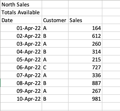
If we were to read the sheet 'North', we would get the following returned:
# Reading a poorly formatted Excel file
import pandas as pd

df = pd.read_excel(
    io='https://github.com/datagy/mediumdata/raw/master/Sales.xlsx',
    sheet_name='North')
print(df.head())

# Returns:
#            North Sales Unnamed: 1 Unnamed: 2
# 0     Totals Available        NaN        NaN
# 1                 Date   Customer      Sales
# 2  2022-04-01 00:00:00          A        164
# 3  2022-04-02 00:00:00          B        612
# 4  2022-04-03 00:00:00          A        260
Pandas makes it easy to skip a certain number of rows when reading an Excel file. This can be done using the skiprows= parameter. We can see that we need to skip two rows, so we can simply pass in the value 2, as shown below:
# Reading a Poorly Formatted File Correctly
import pandas as pd

df = pd.read_excel(
    io='https://github.com/datagy/mediumdata/raw/master/Sales.xlsx',
    sheet_name='North',
    skiprows=2)
print(df.head())

# Returns:
#         Date Customer  Sales
# 0 2022-04-01        A    164
# 1 2022-04-02        B    612
# 2 2022-04-03        A    260
# 3 2022-04-04        B    314
# 4 2022-04-05        A    215
This read the file much more accurately! It can be a lifesaver when working with poorly formatted files. In the next section, you’ll learn how to read multiple sheets in an Excel file in Pandas.
How to Read Multiple Sheets in an Excel File in Pandas
Pandas makes it very easy to read multiple sheets at the same time. This can be done using the sheet_name= parameter. In our earlier examples, we passed in only a single string to read a single sheet. However, you can also pass in a list of sheets to read multiple sheets at once.
Let’s see how we can read our first two sheets:
# Reading Multiple Excel Sheets at Once in Pandas
import pandas as pd

dfs = pd.read_excel(
    io='https://github.com/datagy/mediumdata/raw/master/Sales.xlsx',
    sheet_name=['East', 'West'])

print(type(dfs))

# Returns: <class 'dict'>
In the example above, we passed in a list of sheets to read. When we used the type() function to check the type of the returned value, we saw that a dictionary was returned.
Each of the sheets is a key of the dictionary with the DataFrame being the corresponding key’s value. Let’s see how we can access the 'West' DataFrame:
# Reading Multiple Excel Sheets in Pandas
import pandas as pd

dfs = pd.read_excel(
    io='https://github.com/datagy/mediumdata/raw/master/Sales.xlsx',
    sheet_name=['East', 'West'])

print(dfs.get('West').head())

# Returns:
#         Date Customer  Sales
# 0 2022-04-01        A    504
# 1 2022-04-02        B    361
# 2 2022-04-03        A    694
# 3 2022-04-04        B    702
# 4 2022-04-05        A    255
You can also read all of the sheets at once by specifying None for the value of sheet_name=. Similarly, this returns a dictionary of all sheets:
# Reading Multiple Excel Sheets in Pandas
import pandas as pd

dfs = pd.read_excel(
    io='https://github.com/datagy/mediumdata/raw/master/Sales.xlsx',
    sheet_name=None)
In the next section, you’ll learn how to read multiple Excel files in Pandas.
How to Read Only n Lines When Reading Excel Files in Pandas
When working with very large Excel files, it can be helpful to only sample a small subset of the data first. This allows you to quickly load the file to better be able to explore the different columns and data types.
This can be done using the nrows= parameter, which accepts an integer value of the number of rows you want to read into your DataFrame. Let’s see how we can read the first five rows of the Excel sheet:
# Reading n Number of Rows of an Excel Sheet
import pandas as pd

df = pd.read_excel(
    io='https://github.com/datagy/mediumdata/raw/master/Sales.xlsx',
    nrows=5)
print(df)

# Returns:
#         Date Customer  Sales
# 0 2022-04-01        A    191
# 1 2022-04-02        B    727
# 2 2022-04-03        A    782
# 3 2022-04-04        B    561
# 4 2022-04-05        A    969
Conclusion
In this tutorial, you learned how to use Python and Pandas to read Excel files into a DataFrame using the .read_excel() function. You learned how to use the function to read an Excel, specify sheet names, read only particular columns, and specify data types. You then learned how skip rows, read only a set number of rows, and read multiple sheets.
Additional Resources
To learn more about related topics, check out the tutorials below:
- Pandas Dataframe to CSV File – Export Using .to_csv()
- Combine Data in Pandas with merge, join, and concat
- Introduction to Pandas for Data Science
- Summarizing and Analyzing a Pandas DataFrame
Хотя многие Data Scientist’ы больше привыкли работать с CSV-файлами, на практике очень часто приходится сталкиваться с обычными Excel-таблицами. Поэтому сегодня мы расскажем, как читать Excel-файлы в Pandas, а также рассмотрим основные возможности Python-библиотеки OpenPyXL для чтения метаданных ячеек.
Дополнительные зависимости для возможности чтения Excel таблиц
Для чтения таблиц Excel в Pandas требуются дополнительные зависимости:
- xlrd поддерживает старые и новые форматы MS Excel [1];
- OpenPyXL поддерживает новые форматы MS Excel (.xlsx) [2];
- ODFpy поддерживает свободные форматы OpenDocument (.odf, .ods и .odt) [3];
- pyxlsb поддерживает бинарные MS Excel файлы (формат .xlsb) [4].
Мы рекомендуем установить только OpenPyXL, поскольку он нам пригодится в дальнейшем. Для этого в командной строке прописывается следующая операция:
pip install openpyxl
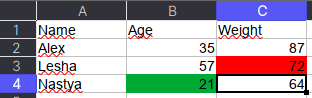
Затем в Pandas нужно указать путь к Excel-файлу и одну из установленных зависимостей. Python-код выглядит следующим образом:
import pandas as pd
pd.read_excel(io='temp1.xlsx', engine='openpyxl')
#
     Name  Age  Weight
0    Alex   35      87
1   Lesha   57      72
2  Nastya   21      64
Читаем несколько листов
Excel-файл может содержать несколько листов. В Pandas, чтобы прочитать конкретный лист, в аргументе нужно указать sheet_name. Можно указать список названий листов, тогда Pandas вернет словарь (dict) с объектами DataFrame:
dfs = pd.read_excel(io='temp1.xlsx',
                    engine='openpyxl',
                    sheet_name=['Sheet1', 'Sheet2'])
dfs
#
{'Sheet1':      Name  Age  Weight
 0    Alex   35      87
 1   Lesha   57      72
 2  Nastya   21      64,
 'Sheet2':     Name  Age  Weight
 0  Gosha   43      95
 1   Anna   24      65
 2   Lena   22      78}
Если таблицы в словаре имеют одинаковые атрибуты, то их можно объединить в один DataFrame. В Python это выглядит так:
pd.concat(dfs).reset_index(drop=True)
     Name  Age  Weight
0    Alex   35      87
1   Lesha   57      72
2  Nastya   21      64
3   Gosha   43      95
4    Anna   24      65
5    Lena   22      78
Указание диапазонов
Таблицы могут размещаться не в самом начале, а как, например, на рисунке ниже. Как видим, таблица располагается в диапазоне A:F.
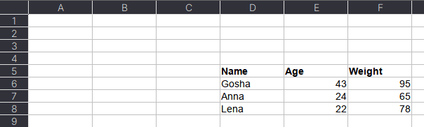
Чтобы прочитать такую таблицу, нужно указать диапазон в аргументе usecols. Также дополнительно можно добавить header — номер заголовка таблицы, а также nrows — количество строк, которые нужно прочитать. В аргументе header всегда передается номер строки на единицу меньше, чем в Excel-файле, поскольку в Python индексация начинается с 0 (на рисунке это номер 5, тогда указываем 4):
pd.read_excel(io='temp1.xlsx',
              engine='openpyxl',
              usecols='D:F',
              header=4, # в excel это №5
              nrows=3)
#
    Name  Age  Weight
0  Gosha   43      95
1   Anna   24      65
2   Lena   22      78
Читаем таблицы в OpenPyXL
Pandas прочитывает только содержимое таблицы, но игнорирует метаданные: цвет заливки ячеек, примечания, стили таблицы и т.д. В таком случае пригодится библиотека OpenPyXL. Загрузка файлов осуществляется через функцию load_workbook, а к листам обращаться можно через квадратные скобки:
from openpyxl import load_workbook
wb = load_workbook('temp2.xlsx')
ws = wb['Лист1']
type(ws)
# openpyxl.worksheet.worksheet.Worksheet
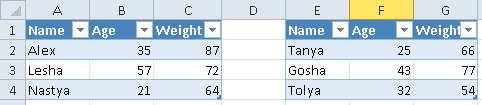
Допустим, имеется Excel-файл с несколькими таблицами на листе (см. рисунок выше). Если бы мы использовали Pandas, то он бы выдал следующий результат:
pd.read_excel(io='temp2.xlsx',
              engine='openpyxl')
#
     Name  Age  Weight  Unnamed: 3 Name.1  Age.1  Weight.1
0    Alex   35      87         NaN  Tanya     25        66
1   Lesha   57      72         NaN  Gosha     43        77
2  Nastya   21      64         NaN  Tolya     32        54
Можно, конечно, заняться обработкой и привести таблицы в нормальный вид, а можно воспользоваться OpenPyXL, который хранит таблицу и его диапазон в словаре. Чтобы посмотреть этот словарь, нужно вызвать ws.tables.items. Вот так выглядит Python-код:
ws.tables.items()
wb = load_workbook('temp2.xlsx')
ws = wb['Лист1']
ws.tables.items()
#
[('Таблица1', 'A1:C4'), ('Таблица13', 'E1:G4')]
Обращаясь к каждому диапазону, можно проходить по каждой строке или столбцу, а внутри них – по каждой ячейке. Например, следующий код на Python таблицы объединяет строки в список, где первая строка уходит на заголовок, а затем преобразует их в DataFrame:
dfs = []
for table_name, value in ws.tables.items():
    table = ws[value]
    header, *body = [[cell.value for cell in row]
                      for row in table]
    df = pd.DataFrame(body, columns=header)
    dfs.append(df)
Если таблицы имеют одинаковые атрибуты, то их можно соединить в одну:
pd.concat(dfs)
#
     Name  Age  Weight
0    Alex   35      87
1   Lesha   57      72
2  Nastya   21      64
0   Tanya   25      66
1   Gosha   43      77
2   Tolya   32      54
Сохраняем метаданные таблицы
Как указано в коде выше, у ячейки OpenPyXL есть атрибут value, который хранит ее значение. Помимо value, можно получить тип ячейки (data_type), цвет заливки (fill), примечание (comment) и др.
Например, требуется сохранить данные о цвете ячеек. Для этого мы каждую ячейку с числами перезапишем в виде <значение,RGB>, где RGB — значение цвета в формате RGB (red, green, blue). Python-код выглядит следующим образом:
# _TYPES = {int:'n', float:'n', str:'s', bool:'b'}
data = []
for row in ws.rows:
    row_cells = []
    for cell in row:
        cell_value = cell.value
        if cell.data_type == 'n':
            cell_value = f"{cell_value},{cell.fill.fgColor.rgb}"
        row_cells.append(cell_value)
    data.append(row_cells)
Первым элементом списка является строка-заголовок, а все остальное уже значения таблицы:
pd.DataFrame(data[1:], columns=data[0])
#
     Name          Age       Weight
0    Alex  35,00000000  87,00000000
1   Lesha  57,00000000  72,FFFF0000
2  Nastya  21,FF00A933  64,00000000
Теперь представим атрибуты в виде индексов с помощью метода stack, а после разобьём все записи на значение и цвет методом str.split:
(pd.DataFrame(data[1:], columns=data[0])
 .set_index('Name')
 .stack()
 .str.split(',', expand=True)
)
#
                0         1
Name
Alex   Age     35  00000000
       Weight  87  00000000
Lesha  Age     57  00000000
       Weight  72  FFFF0000
Nastya Age     21  FF00A933
       Weight  64  0000000
Осталось только переименовать 0 и 1 на Value и Color, а также добавить атрибут Variable, который обозначит Вес и Возраст. Полный код на Python выглядит следующим образом:
(pd.DataFrame(data[1:], columns=data[0])
 .set_index('Name')
 .stack()
 .str.split(',', expand=True)
 .set_axis(['Value', 'Color'], axis=1)
 .rename_axis(index=['Name', 'Variable'])
 .reset_index()
)
#
     Name Variable Value     Color
0    Alex      Age    35  00000000
1    Alex   Weight    87  00000000
2   Lesha      Age    57  00000000
3   Lesha   Weight    72  FFFF0000
4  Nastya      Age    21  FF00A933
5  Nastya   Weight    64  00000000
Ещё больше подробностей о работе с таблицами в Pandas, а также их обработке на реальных примерах Data Science задач, вы узнаете на наших курсах по Python в лицензированном учебном центре обучения и повышения квалификации IT-специалистов в Москве.
Источники
- https://xlrd.readthedocs.io/en/latest/
- https://openpyxl.readthedocs.io/en/latest/
- https://github.com/eea/odfpy
- https://github.com/willtrnr/pyxlsb
Watch Now This tutorial has a related video course created by the Real Python team. Watch it together with the written tutorial to deepen your understanding: Reading and Writing Files With Pandas
pandas is a powerful and flexible Python package that allows you to work with labeled and time series data. It also provides statistics methods, enables plotting, and more. One crucial feature of pandas is its ability to write and read Excel, CSV, and many other types of files. Functions like the pandas read_csv() method enable you to work with files effectively. You can use them to save the data and labels from pandas objects to a file and load them later as pandas Series or DataFrame instances.
In this tutorial, you’ll learn:
- What the pandas IO tools API is
- How to read and write data to and from files
- How to work with various file formats
- How to work with big data efficiently
Let’s start reading and writing files!
Installing pandas
The code in this tutorial is executed with CPython 3.7.4 and pandas 0.25.1. It would be beneficial to make sure you have the latest versions of Python and pandas on your machine. You might want to create a new virtual environment and install the dependencies for this tutorial.
First, you’ll need the pandas library. You may already have it installed. If you don’t, then you can install it with pip:
Once the installation process completes, you should have pandas installed and ready.
Anaconda is an excellent Python distribution that comes with Python, many useful packages like pandas, and a package and environment manager called Conda. To learn more about Anaconda, check out Setting Up Python for Machine Learning on Windows.
If you don’t have pandas in your virtual environment, then you can install it with Conda:
Conda is powerful as it manages the dependencies and their versions. To learn more about working with Conda, you can check out the official documentation.
Preparing Data
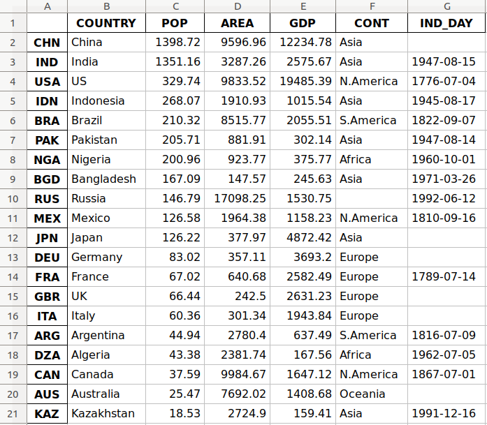
In this tutorial, you’ll use the data related to 20 countries. Here’s an overview of the data and sources you’ll be working with:
-
Country is denoted by the country name. Each country is in the top 10 list for either population, area, or gross domestic product (GDP). The row labels for the dataset are the three-letter country codes defined in ISO 3166-1. The column label for the dataset is
COUNTRY. -
Population is expressed in millions. The data comes from a list of countries and dependencies by population on Wikipedia. The column label for the dataset is
POP. -
Area is expressed in thousands of kilometers squared. The data comes from a list of countries and dependencies by area on Wikipedia. The column label for the dataset is
AREA. -
Gross domestic product is expressed in millions of U.S. dollars, according to the United Nations data for 2017. You can find this data in the list of countries by nominal GDP on Wikipedia. The column label for the dataset is
GDP. -
Continent is either Africa, Asia, Oceania, Europe, North America, or South America. You can find this information on Wikipedia as well. The column label for the dataset is
CONT. -
Independence day is a date that commemorates a nation’s independence. The data comes from the list of national independence days on Wikipedia. The dates are shown in ISO 8601 format. The first four digits represent the year, the next two numbers are the month, and the last two are for the day of the month. The column label for the dataset is
IND_DAY.
This is how the data looks as a table:
| COUNTRY | POP | AREA | GDP | CONT | IND_DAY | |
|---|---|---|---|---|---|---|
| CHN | China | 1398.72 | 9596.96 | 12234.78 | Asia | |
| IND | India | 1351.16 | 3287.26 | 2575.67 | Asia | 1947-08-15 |
| USA | US | 329.74 | 9833.52 | 19485.39 | N.America | 1776-07-04 |
| IDN | Indonesia | 268.07 | 1910.93 | 1015.54 | Asia | 1945-08-17 |
| BRA | Brazil | 210.32 | 8515.77 | 2055.51 | S.America | 1822-09-07 |
| PAK | Pakistan | 205.71 | 881.91 | 302.14 | Asia | 1947-08-14 |
| NGA | Nigeria | 200.96 | 923.77 | 375.77 | Africa | 1960-10-01 |
| BGD | Bangladesh | 167.09 | 147.57 | 245.63 | Asia | 1971-03-26 |
| RUS | Russia | 146.79 | 17098.25 | 1530.75 | 1992-06-12 | |
| MEX | Mexico | 126.58 | 1964.38 | 1158.23 | N.America | 1810-09-16 |
| JPN | Japan | 126.22 | 377.97 | 4872.42 | Asia | |
| DEU | Germany | 83.02 | 357.11 | 3693.20 | Europe | |
| FRA | France | 67.02 | 640.68 | 2582.49 | Europe | 1789-07-14 |
| GBR | UK | 66.44 | 242.50 | 2631.23 | Europe | |
| ITA | Italy | 60.36 | 301.34 | 1943.84 | Europe | |
| ARG | Argentina | 44.94 | 2780.40 | 637.49 | S.America | 1816-07-09 |
| DZA | Algeria | 43.38 | 2381.74 | 167.56 | Africa | 1962-07-05 |
| CAN | Canada | 37.59 | 9984.67 | 1647.12 | N.America | 1867-07-01 |
| AUS | Australia | 25.47 | 7692.02 | 1408.68 | Oceania | |
| KAZ | Kazakhstan | 18.53 | 2724.90 | 159.41 | Asia | 1991-12-16 |
You may notice that some of the data is missing. For example, the continent for Russia is not specified because it spreads across both Europe and Asia. There are also several missing independence days because the data source omits them.
You can organize this data in Python using a nested dictionary:
data = {
    'CHN': {'COUNTRY': 'China', 'POP': 1_398.72, 'AREA': 9_596.96,
            'GDP': 12_234.78, 'CONT': 'Asia'},
    'IND': {'COUNTRY': 'India', 'POP': 1_351.16, 'AREA': 3_287.26,
            'GDP': 2_575.67, 'CONT': 'Asia', 'IND_DAY': '1947-08-15'},
    'USA': {'COUNTRY': 'US', 'POP': 329.74, 'AREA': 9_833.52,
            'GDP': 19_485.39, 'CONT': 'N.America',
            'IND_DAY': '1776-07-04'},
    'IDN': {'COUNTRY': 'Indonesia', 'POP': 268.07, 'AREA': 1_910.93,
            'GDP': 1_015.54, 'CONT': 'Asia', 'IND_DAY': '1945-08-17'},
    'BRA': {'COUNTRY': 'Brazil', 'POP': 210.32, 'AREA': 8_515.77,
            'GDP': 2_055.51, 'CONT': 'S.America', 'IND_DAY': '1822-09-07'},
    'PAK': {'COUNTRY': 'Pakistan', 'POP': 205.71, 'AREA': 881.91,
            'GDP': 302.14, 'CONT': 'Asia', 'IND_DAY': '1947-08-14'},
    'NGA': {'COUNTRY': 'Nigeria', 'POP': 200.96, 'AREA': 923.77,
            'GDP': 375.77, 'CONT': 'Africa', 'IND_DAY': '1960-10-01'},
    'BGD': {'COUNTRY': 'Bangladesh', 'POP': 167.09, 'AREA': 147.57,
            'GDP': 245.63, 'CONT': 'Asia', 'IND_DAY': '1971-03-26'},
    'RUS': {'COUNTRY': 'Russia', 'POP': 146.79, 'AREA': 17_098.25,
            'GDP': 1_530.75, 'IND_DAY': '1992-06-12'},
    'MEX': {'COUNTRY': 'Mexico', 'POP': 126.58, 'AREA': 1_964.38,
            'GDP': 1_158.23, 'CONT': 'N.America', 'IND_DAY': '1810-09-16'},
    'JPN': {'COUNTRY': 'Japan', 'POP': 126.22, 'AREA': 377.97,
            'GDP': 4_872.42, 'CONT': 'Asia'},
    'DEU': {'COUNTRY': 'Germany', 'POP': 83.02, 'AREA': 357.11,
            'GDP': 3_693.20, 'CONT': 'Europe'},
    'FRA': {'COUNTRY': 'France', 'POP': 67.02, 'AREA': 640.68,
            'GDP': 2_582.49, 'CONT': 'Europe', 'IND_DAY': '1789-07-14'},
    'GBR': {'COUNTRY': 'UK', 'POP': 66.44, 'AREA': 242.50,
            'GDP': 2_631.23, 'CONT': 'Europe'},
    'ITA': {'COUNTRY': 'Italy', 'POP': 60.36, 'AREA': 301.34,
            'GDP': 1_943.84, 'CONT': 'Europe'},
    'ARG': {'COUNTRY': 'Argentina', 'POP': 44.94, 'AREA': 2_780.40,
            'GDP': 637.49, 'CONT': 'S.America', 'IND_DAY': '1816-07-09'},
    'DZA': {'COUNTRY': 'Algeria', 'POP': 43.38, 'AREA': 2_381.74,
            'GDP': 167.56, 'CONT': 'Africa', 'IND_DAY': '1962-07-05'},
    'CAN': {'COUNTRY': 'Canada', 'POP': 37.59, 'AREA': 9_984.67,
            'GDP': 1_647.12, 'CONT': 'N.America', 'IND_DAY': '1867-07-01'},
    'AUS': {'COUNTRY': 'Australia', 'POP': 25.47, 'AREA': 7_692.02,
            'GDP': 1_408.68, 'CONT': 'Oceania'},
    'KAZ': {'COUNTRY': 'Kazakhstan', 'POP': 18.53, 'AREA': 2_724.90,
            'GDP': 159.41, 'CONT': 'Asia', 'IND_DAY': '1991-12-16'}
}

columns = ('COUNTRY', 'POP', 'AREA', 'GDP', 'CONT', 'IND_DAY')
Each row of the table is written as an inner dictionary whose keys are the column names and values are the corresponding data. These dictionaries are then collected as the values in the outer data dictionary. The corresponding keys for data are the three-letter country codes.
You can use this data to create an instance of a pandas DataFrame. First, you need to import pandas:
>>>
>>> import pandas as pd
Now that you have pandas imported, you can use the DataFrame constructor and data to create a DataFrame object.
data is organized in such a way that the country codes correspond to columns. You can reverse the rows and columns of a DataFrame with the property .T:
>>>
>>> df = pd.DataFrame(data=data).T
>>> df
        COUNTRY      POP     AREA      GDP       CONT     IND_DAY
CHN       China  1398.72  9596.96  12234.8       Asia         NaN
IND       India  1351.16  3287.26  2575.67       Asia  1947-08-15
USA          US   329.74  9833.52  19485.4  N.America  1776-07-04
IDN   Indonesia   268.07  1910.93  1015.54       Asia  1945-08-17
BRA      Brazil   210.32  8515.77  2055.51  S.America  1822-09-07
PAK    Pakistan   205.71   881.91   302.14       Asia  1947-08-14
NGA     Nigeria   200.96   923.77   375.77     Africa  1960-10-01
BGD  Bangladesh   167.09   147.57   245.63       Asia  1971-03-26
RUS      Russia   146.79  17098.2  1530.75        NaN  1992-06-12
MEX      Mexico   126.58  1964.38  1158.23  N.America  1810-09-16
JPN       Japan   126.22   377.97  4872.42       Asia         NaN
DEU     Germany    83.02   357.11   3693.2     Europe         NaN
FRA      France    67.02   640.68  2582.49     Europe  1789-07-14
GBR          UK    66.44    242.5  2631.23     Europe         NaN
ITA       Italy    60.36   301.34  1943.84     Europe         NaN
ARG   Argentina    44.94   2780.4   637.49  S.America  1816-07-09
DZA     Algeria    43.38  2381.74   167.56     Africa  1962-07-05
CAN      Canada    37.59  9984.67  1647.12  N.America  1867-07-01
AUS   Australia    25.47  7692.02  1408.68    Oceania         NaN
KAZ  Kazakhstan    18.53   2724.9   159.41       Asia  1991-12-16
Now you have your DataFrame object populated with the data about each country.
Versions of Python older than 3.6 did not guarantee the order of keys in dictionaries. To ensure the order of columns is maintained for older versions of Python and pandas, you can specify index=columns:
>>>
>>> df = pd.DataFrame(data=data, index=columns).T
Now that you’ve prepared your data, you’re ready to start working with files!
Using the pandas read_csv() and .to_csv() Functions
A comma-separated values (CSV) file is a plaintext file with a .csv extension that holds tabular data. This is one of the most popular file formats for storing large amounts of data. Each row of the CSV file represents a single table row. The values in the same row are by default separated with commas, but you could change the separator to a semicolon, tab, space, or some other character.
Write a CSV File
You can save your pandas DataFrame as a CSV file with .to_csv():
>>>
>>> df.to_csv('data.csv')
That’s it! You’ve created the file data.csv in your current working directory. You can expand the code block below to see how your CSV file should look:
,COUNTRY,POP,AREA,GDP,CONT,IND_DAY
CHN,China,1398.72,9596.96,12234.78,Asia,
IND,India,1351.16,3287.26,2575.67,Asia,1947-08-15
USA,US,329.74,9833.52,19485.39,N.America,1776-07-04
IDN,Indonesia,268.07,1910.93,1015.54,Asia,1945-08-17
BRA,Brazil,210.32,8515.77,2055.51,S.America,1822-09-07
PAK,Pakistan,205.71,881.91,302.14,Asia,1947-08-14
NGA,Nigeria,200.96,923.77,375.77,Africa,1960-10-01
BGD,Bangladesh,167.09,147.57,245.63,Asia,1971-03-26
RUS,Russia,146.79,17098.25,1530.75,,1992-06-12
MEX,Mexico,126.58,1964.38,1158.23,N.America,1810-09-16
JPN,Japan,126.22,377.97,4872.42,Asia,
DEU,Germany,83.02,357.11,3693.2,Europe,
FRA,France,67.02,640.68,2582.49,Europe,1789-07-14
GBR,UK,66.44,242.5,2631.23,Europe,
ITA,Italy,60.36,301.34,1943.84,Europe,
ARG,Argentina,44.94,2780.4,637.49,S.America,1816-07-09
DZA,Algeria,43.38,2381.74,167.56,Africa,1962-07-05
CAN,Canada,37.59,9984.67,1647.12,N.America,1867-07-01
AUS,Australia,25.47,7692.02,1408.68,Oceania,
KAZ,Kazakhstan,18.53,2724.9,159.41,Asia,1991-12-16
This text file contains the data separated with commas. The first column contains the row labels. In some cases, you’ll find them irrelevant. If you don’t want to keep them, then you can pass the argument index=False to .to_csv().
Read a CSV File
Once your data is saved in a CSV file, you’ll likely want to load and use it from time to time. You can do that with the pandas read_csv() function:
>>>
>>> df = pd.read_csv('data.csv', index_col=0)
>>> df
        COUNTRY      POP      AREA       GDP       CONT     IND_DAY
CHN       China  1398.72   9596.96  12234.78       Asia         NaN
IND       India  1351.16   3287.26   2575.67       Asia  1947-08-15
USA          US   329.74   9833.52  19485.39  N.America  1776-07-04
IDN   Indonesia   268.07   1910.93   1015.54       Asia  1945-08-17
BRA      Brazil   210.32   8515.77   2055.51  S.America  1822-09-07
PAK    Pakistan   205.71    881.91    302.14       Asia  1947-08-14
NGA     Nigeria   200.96    923.77    375.77     Africa  1960-10-01
BGD  Bangladesh   167.09    147.57    245.63       Asia  1971-03-26
RUS      Russia   146.79  17098.25   1530.75        NaN  1992-06-12
MEX      Mexico   126.58   1964.38   1158.23  N.America  1810-09-16
JPN       Japan   126.22    377.97   4872.42       Asia         NaN
DEU     Germany    83.02    357.11   3693.20     Europe         NaN
FRA      France    67.02    640.68   2582.49     Europe  1789-07-14
GBR          UK    66.44    242.50   2631.23     Europe         NaN
ITA       Italy    60.36    301.34   1943.84     Europe         NaN
ARG   Argentina    44.94   2780.40    637.49  S.America  1816-07-09
DZA     Algeria    43.38   2381.74    167.56     Africa  1962-07-05
CAN      Canada    37.59   9984.67   1647.12  N.America  1867-07-01
AUS   Australia    25.47   7692.02   1408.68    Oceania         NaN
KAZ  Kazakhstan    18.53   2724.90    159.41       Asia  1991-12-16
In this case, the pandas read_csv() function returns a new DataFrame with the data and labels from the file data.csv, which you specified with the first argument. This string can be any valid path, including URLs.
The parameter index_col specifies the column from the CSV file that contains the row labels. You assign a zero-based column index to this parameter. You should determine the value of index_col when the CSV file contains the row labels to avoid loading them as data.
You’ll learn more about using pandas with CSV files later on in this tutorial. You can also check out Reading and Writing CSV Files in Python to see how to handle CSV files with the built-in Python library csv as well.
Using pandas to Write and Read Excel Files
Microsoft Excel is probably the most widely-used spreadsheet software. While older versions used binary .xls files, Excel 2007 introduced the new XML-based .xlsx file. You can read and write Excel files in pandas, similar to CSV files. However, you’ll need to install the following Python packages first:
- xlwt to write to
.xlsfiles - openpyxl or XlsxWriter to write to
.xlsxfiles - xlrd to read Excel files
You can install them using pip with a single command:
$ pip install xlwt openpyxl xlsxwriter xlrd
You can also use Conda:
$ conda install xlwt openpyxl xlsxwriter xlrd
Please note that you don’t have to install all these packages. For example, you don’t need both openpyxl and XlsxWriter. If you’re going to work just with .xls files, then you don’t need any of them! However, if you intend to work only with .xlsx files, then you’re going to need at least one of them, but not xlwt. Take some time to decide which packages are right for your project.
Write an Excel File
Once you have those packages installed, you can save your DataFrame in an Excel file with .to_excel():
>>>
>>> df.to_excel('data.xlsx')
The argument 'data.xlsx' represents the target file and, optionally, its path. The above statement should create the file data.xlsx in your current working directory. That file should look like this:
The first column of the file contains the labels of the rows, while the other columns store data.
Read an Excel File
You can load data from Excel files with read_excel():
>>>
>>> df = pd.read_excel('data.xlsx', index_col=0)
>>> df
        COUNTRY      POP      AREA       GDP       CONT     IND_DAY
CHN       China  1398.72   9596.96  12234.78       Asia         NaN
IND       India  1351.16   3287.26   2575.67       Asia  1947-08-15
USA          US   329.74   9833.52  19485.39  N.America  1776-07-04
IDN   Indonesia   268.07   1910.93   1015.54       Asia  1945-08-17
BRA      Brazil   210.32   8515.77   2055.51  S.America  1822-09-07
PAK    Pakistan   205.71    881.91    302.14       Asia  1947-08-14
NGA     Nigeria   200.96    923.77    375.77     Africa  1960-10-01
BGD  Bangladesh   167.09    147.57    245.63       Asia  1971-03-26
RUS      Russia   146.79  17098.25   1530.75        NaN  1992-06-12
MEX      Mexico   126.58   1964.38   1158.23  N.America  1810-09-16
JPN       Japan   126.22    377.97   4872.42       Asia         NaN
DEU     Germany    83.02    357.11   3693.20     Europe         NaN
FRA      France    67.02    640.68   2582.49     Europe  1789-07-14
GBR          UK    66.44    242.50   2631.23     Europe         NaN
ITA       Italy    60.36    301.34   1943.84     Europe         NaN
ARG   Argentina    44.94   2780.40    637.49  S.America  1816-07-09
DZA     Algeria    43.38   2381.74    167.56     Africa  1962-07-05
CAN      Canada    37.59   9984.67   1647.12  N.America  1867-07-01
AUS   Australia    25.47   7692.02   1408.68    Oceania         NaN
KAZ  Kazakhstan    18.53   2724.90    159.41       Asia  1991-12-16
read_excel() returns a new DataFrame that contains the values from data.xlsx. You can also use read_excel() with OpenDocument spreadsheets, or .ods files.
You’ll learn more about working with Excel files later on in this tutorial. You can also check out Using pandas to Read Large Excel Files in Python.
Understanding the pandas IO API
pandas IO Tools is the API that allows you to save the contents of Series and DataFrame objects to the clipboard, objects, or files of various types. It also enables loading data from the clipboard, objects, or files.
Write Files
Series and DataFrame objects have methods that enable writing data and labels to the clipboard or files. They’re named with the pattern .to_<file-type>(), where <file-type> is the type of the target file.
You’ve learned about .to_csv() and .to_excel(), but there are others, including:
.to_json().to_html().to_sql().to_pickle()
There are still more file types that you can write to, so this list is not exhaustive.
These methods have parameters specifying the target file path where you saved the data and labels. This is mandatory in some cases and optional in others. If this option is available and you choose to omit it, then the methods return the objects (like strings or iterables) with the contents of DataFrame instances.
The optional parameter compression decides how to compress the file with the data and labels. You’ll learn more about it later on. There are a few other parameters, but they’re mostly specific to one or several methods. You won’t go into them in detail here.
Read Files
pandas functions for reading the contents of files are named using the pattern .read_<file-type>(), where <file-type> indicates the type of the file to read. You’ve already seen the pandas read_csv() and read_excel() functions. Here are a few others:
read_json()read_html()read_sql()read_pickle()
These functions have a parameter that specifies the target file path. It can be any valid string that represents the path, either on a local machine or in a URL. Other objects are also acceptable depending on the file type.
The optional parameter compression determines the type of decompression to use for the compressed files. You’ll learn about it later on in this tutorial. There are other parameters, but they’re specific to one or several functions. You won’t go into them in detail here.
Working With Different File Types
The pandas library offers a wide range of possibilities for saving your data to files and loading data from files. In this section, you’ll learn more about working with CSV and Excel files. You’ll also see how to use other types of files, like JSON, web pages, databases, and Python pickle files.
CSV Files
You’ve already learned how to read and write CSV files. Now let’s dig a little deeper into the details. When you use .to_csv() to save your DataFrame, you can provide an argument for the parameter path_or_buf to specify the path, name, and extension of the target file.
path_or_buf is the first argument .to_csv() will get. It can be any string that represents a valid file path that includes the file name and its extension. You’ve seen this in a previous example. However, if you omit path_or_buf, then .to_csv() won’t create any files. Instead, it’ll return the corresponding string:
>>>
>>> df = pd.DataFrame(data=data).T
>>> s = df.to_csv()
>>> print(s)
,COUNTRY,POP,AREA,GDP,CONT,IND_DAY
CHN,China,1398.72,9596.96,12234.78,Asia,
IND,India,1351.16,3287.26,2575.67,Asia,1947-08-15
USA,US,329.74,9833.52,19485.39,N.America,1776-07-04
IDN,Indonesia,268.07,1910.93,1015.54,Asia,1945-08-17
BRA,Brazil,210.32,8515.77,2055.51,S.America,1822-09-07
PAK,Pakistan,205.71,881.91,302.14,Asia,1947-08-14
NGA,Nigeria,200.96,923.77,375.77,Africa,1960-10-01
BGD,Bangladesh,167.09,147.57,245.63,Asia,1971-03-26
RUS,Russia,146.79,17098.25,1530.75,,1992-06-12
MEX,Mexico,126.58,1964.38,1158.23,N.America,1810-09-16
JPN,Japan,126.22,377.97,4872.42,Asia,
DEU,Germany,83.02,357.11,3693.2,Europe,
FRA,France,67.02,640.68,2582.49,Europe,1789-07-14
GBR,UK,66.44,242.5,2631.23,Europe,
ITA,Italy,60.36,301.34,1943.84,Europe,
ARG,Argentina,44.94,2780.4,637.49,S.America,1816-07-09
DZA,Algeria,43.38,2381.74,167.56,Africa,1962-07-05
CAN,Canada,37.59,9984.67,1647.12,N.America,1867-07-01
AUS,Australia,25.47,7692.02,1408.68,Oceania,
KAZ,Kazakhstan,18.53,2724.9,159.41,Asia,1991-12-16
Now you have the string s instead of a CSV file. You also have some missing values in your DataFrame object. For example, the continent for Russia and the independence days for several countries (China, Japan, and so on) are not available. In data science and machine learning, you must handle missing values carefully. pandas excels here! By default, pandas uses the NaN value to replace the missing values.
The continent that corresponds to Russia in df is nan:
>>>
>>> df.loc['RUS', 'CONT']
nan
This example uses .loc[] to get data with the specified row and column names.
When you save your DataFrame to a CSV file, empty strings ('') will represent the missing data. You can see this both in your file data.csv and in the string s. If you want to change this behavior, then use the optional parameter na_rep:
>>>
>>> df.to_csv('new-data.csv', na_rep='(missing)')
This code produces the file new-data.csv where the missing values are no longer empty strings. You can expand the code block below to see how this file should look:
,COUNTRY,POP,AREA,GDP,CONT,IND_DAY
CHN,China,1398.72,9596.96,12234.78,Asia,(missing)
IND,India,1351.16,3287.26,2575.67,Asia,1947-08-15
USA,US,329.74,9833.52,19485.39,N.America,1776-07-04
IDN,Indonesia,268.07,1910.93,1015.54,Asia,1945-08-17
BRA,Brazil,210.32,8515.77,2055.51,S.America,1822-09-07
PAK,Pakistan,205.71,881.91,302.14,Asia,1947-08-14
NGA,Nigeria,200.96,923.77,375.77,Africa,1960-10-01
BGD,Bangladesh,167.09,147.57,245.63,Asia,1971-03-26
RUS,Russia,146.79,17098.25,1530.75,(missing),1992-06-12
MEX,Mexico,126.58,1964.38,1158.23,N.America,1810-09-16
JPN,Japan,126.22,377.97,4872.42,Asia,(missing)
DEU,Germany,83.02,357.11,3693.2,Europe,(missing)
FRA,France,67.02,640.68,2582.49,Europe,1789-07-14
GBR,UK,66.44,242.5,2631.23,Europe,(missing)
ITA,Italy,60.36,301.34,1943.84,Europe,(missing)
ARG,Argentina,44.94,2780.4,637.49,S.America,1816-07-09
DZA,Algeria,43.38,2381.74,167.56,Africa,1962-07-05
CAN,Canada,37.59,9984.67,1647.12,N.America,1867-07-01
AUS,Australia,25.47,7692.02,1408.68,Oceania,(missing)
KAZ,Kazakhstan,18.53,2724.9,159.41,Asia,1991-12-16
Now, the string '(missing)' in the file corresponds to the nan values from df.
When pandas reads files, it considers the empty string ('') and a few others as missing values by default:
'nan''-nan''NA''N/A''NaN''null'
If you don’t want this behavior, then you can pass keep_default_na=False to the pandas read_csv() function. To specify other labels for missing values, use the parameter na_values:
>>>
>>> pd.read_csv('new-data.csv', index_col=0, na_values='(missing)')
        COUNTRY      POP      AREA       GDP       CONT     IND_DAY
CHN       China  1398.72   9596.96  12234.78       Asia         NaN
IND       India  1351.16   3287.26   2575.67       Asia  1947-08-15
USA          US   329.74   9833.52  19485.39  N.America  1776-07-04
IDN   Indonesia   268.07   1910.93   1015.54       Asia  1945-08-17
BRA      Brazil   210.32   8515.77   2055.51  S.America  1822-09-07
PAK    Pakistan   205.71    881.91    302.14       Asia  1947-08-14
NGA     Nigeria   200.96    923.77    375.77     Africa  1960-10-01
BGD  Bangladesh   167.09    147.57    245.63       Asia  1971-03-26
RUS      Russia   146.79  17098.25   1530.75        NaN  1992-06-12
MEX      Mexico   126.58   1964.38   1158.23  N.America  1810-09-16
JPN       Japan   126.22    377.97   4872.42       Asia         NaN
DEU     Germany    83.02    357.11   3693.20     Europe         NaN
FRA      France    67.02    640.68   2582.49     Europe  1789-07-14
GBR          UK    66.44    242.50   2631.23     Europe         NaN
ITA       Italy    60.36    301.34   1943.84     Europe         NaN
ARG   Argentina    44.94   2780.40    637.49  S.America  1816-07-09
DZA     Algeria    43.38   2381.74    167.56     Africa  1962-07-05
CAN      Canada    37.59   9984.67   1647.12  N.America  1867-07-01
AUS   Australia    25.47   7692.02   1408.68    Oceania         NaN
KAZ  Kazakhstan    18.53   2724.90    159.41       Asia  1991-12-16
Here, you’ve marked the string '(missing)' as a new missing data label, and pandas replaced it with nan when it read the file.
When you load data from a file, pandas assigns the data types to the values of each column by default. You can check these types with .dtypes:
>>>
>>> df = pd.read_csv('data.csv', index_col=0)
>>> df.dtypes
COUNTRY     object
POP        float64
AREA       float64
GDP        float64
CONT        object
IND_DAY     object
dtype: object
The columns with strings and dates ('COUNTRY', 'CONT', and 'IND_DAY') have the data type object. Meanwhile, the numeric columns contain 64-bit floating-point numbers (float64).
You can use the parameter dtype to specify the desired data types and parse_dates to force use of datetimes:
>>>
>>> dtypes = {'POP': 'float32', 'AREA': 'float32', 'GDP': 'float32'}
>>> df = pd.read_csv('data.csv', index_col=0, dtype=dtypes,
...                  parse_dates=['IND_DAY'])
>>> df.dtypes
COUNTRY            object
POP               float32
AREA              float32
GDP               float32
CONT               object
IND_DAY    datetime64[ns]
dtype: object
>>> df['IND_DAY']
CHN          NaT
IND   1947-08-15
USA   1776-07-04
IDN   1945-08-17
BRA   1822-09-07
PAK   1947-08-14
NGA   1960-10-01
BGD   1971-03-26
RUS   1992-06-12
MEX   1810-09-16
JPN          NaT
DEU          NaT
FRA   1789-07-14
GBR          NaT
ITA          NaT
ARG   1816-07-09
DZA   1962-07-05
CAN   1867-07-01
AUS          NaT
KAZ   1991-12-16
Name: IND_DAY, dtype: datetime64[ns]
Now, you have 32-bit floating-point numbers (float32) as specified with dtype. These differ slightly from the original 64-bit numbers because of smaller precision. The values in the last column are considered as dates and have the data type datetime64. That’s why the NaN values in this column are replaced with NaT.
Now that you have real dates, you can save them in the format you like:
>>>
>>> df = pd.read_csv('data.csv', index_col=0, parse_dates=['IND_DAY'])
>>> df.to_csv('formatted-data.csv', date_format='%B %d, %Y')
Here, you’ve specified the parameter date_format to be '%B %d, %Y'. You can expand the code block below to see the resulting file:
,COUNTRY,POP,AREA,GDP,CONT,IND_DAY
CHN,China,1398.72,9596.96,12234.78,Asia,
IND,India,1351.16,3287.26,2575.67,Asia,"August 15, 1947"
USA,US,329.74,9833.52,19485.39,N.America,"July 04, 1776"
IDN,Indonesia,268.07,1910.93,1015.54,Asia,"August 17, 1945"
BRA,Brazil,210.32,8515.77,2055.51,S.America,"September 07, 1822"
PAK,Pakistan,205.71,881.91,302.14,Asia,"August 14, 1947"
NGA,Nigeria,200.96,923.77,375.77,Africa,"October 01, 1960"
BGD,Bangladesh,167.09,147.57,245.63,Asia,"March 26, 1971"
RUS,Russia,146.79,17098.25,1530.75,,"June 12, 1992"
MEX,Mexico,126.58,1964.38,1158.23,N.America,"September 16, 1810"
JPN,Japan,126.22,377.97,4872.42,Asia,
DEU,Germany,83.02,357.11,3693.2,Europe,
FRA,France,67.02,640.68,2582.49,Europe,"July 14, 1789"
GBR,UK,66.44,242.5,2631.23,Europe,
ITA,Italy,60.36,301.34,1943.84,Europe,
ARG,Argentina,44.94,2780.4,637.49,S.America,"July 09, 1816"
DZA,Algeria,43.38,2381.74,167.56,Africa,"July 05, 1962"
CAN,Canada,37.59,9984.67,1647.12,N.America,"July 01, 1867"
AUS,Australia,25.47,7692.02,1408.68,Oceania,
KAZ,Kazakhstan,18.53,2724.9,159.41,Asia,"December 16, 1991"
The format of the dates is different now. The format '%B %d, %Y' means the date will first display the full name of the month, then the day followed by a comma, and finally the full year.
There are several other optional parameters that you can use with .to_csv():
sepdenotes a values separator.decimalindicates a decimal separator.encodingsets the file encoding.headerspecifies whether you want to write column labels in the file.
Here’s how you would pass arguments for sep and header:
>>>
>>> s = df.to_csv(sep=';', header=False)
>>> print(s)
CHN;China;1398.72;9596.96;12234.78;Asia;
IND;India;1351.16;3287.26;2575.67;Asia;1947-08-15
USA;US;329.74;9833.52;19485.39;N.America;1776-07-04
IDN;Indonesia;268.07;1910.93;1015.54;Asia;1945-08-17
BRA;Brazil;210.32;8515.77;2055.51;S.America;1822-09-07
PAK;Pakistan;205.71;881.91;302.14;Asia;1947-08-14
NGA;Nigeria;200.96;923.77;375.77;Africa;1960-10-01
BGD;Bangladesh;167.09;147.57;245.63;Asia;1971-03-26
RUS;Russia;146.79;17098.25;1530.75;;1992-06-12
MEX;Mexico;126.58;1964.38;1158.23;N.America;1810-09-16
JPN;Japan;126.22;377.97;4872.42;Asia;
DEU;Germany;83.02;357.11;3693.2;Europe;
FRA;France;67.02;640.68;2582.49;Europe;1789-07-14
GBR;UK;66.44;242.5;2631.23;Europe;
ITA;Italy;60.36;301.34;1943.84;Europe;
ARG;Argentina;44.94;2780.4;637.49;S.America;1816-07-09
DZA;Algeria;43.38;2381.74;167.56;Africa;1962-07-05
CAN;Canada;37.59;9984.67;1647.12;N.America;1867-07-01
AUS;Australia;25.47;7692.02;1408.68;Oceania;
KAZ;Kazakhstan;18.53;2724.9;159.41;Asia;1991-12-16
The data is separated with a semicolon (';') because you’ve specified sep=';'. Also, since you passed header=False, you see your data without the header row of column names.
The pandas read_csv() function has many additional options for managing missing data, working with dates and times, quoting, encoding, handling errors, and more. For instance, if you have a file with one data column and want to get a Series object instead of a DataFrame, then you can pass squeeze=True to read_csv(). You’ll learn later on about data compression and decompression, as well as how to skip rows and columns.
JSON Files
JSON stands for JavaScript object notation. JSON files are plaintext files used for data interchange, and humans can read them easily. They follow the ISO/IEC 21778:2017 and ECMA-404 standards and use the .json extension. Python and pandas work well with JSON files, as Python’s json library offers built-in support for them.
You can save the data from your DataFrame to a JSON file with .to_json(). Start by creating a DataFrame object again. Use the dictionary data that holds the data about countries and then apply .to_json():
>>>
>>> df = pd.DataFrame(data=data).T
>>> df.to_json('data-columns.json')
This code produces the file data-columns.json. You can expand the code block below to see how this file should look:
{"COUNTRY":{"CHN":"China","IND":"India","USA":"US","IDN":"Indonesia","BRA":"Brazil","PAK":"Pakistan","NGA":"Nigeria","BGD":"Bangladesh","RUS":"Russia","MEX":"Mexico","JPN":"Japan","DEU":"Germany","FRA":"France","GBR":"UK","ITA":"Italy","ARG":"Argentina","DZA":"Algeria","CAN":"Canada","AUS":"Australia","KAZ":"Kazakhstan"},"POP":{"CHN":1398.72,"IND":1351.16,"USA":329.74,"IDN":268.07,"BRA":210.32,"PAK":205.71,"NGA":200.96,"BGD":167.09,"RUS":146.79,"MEX":126.58,"JPN":126.22,"DEU":83.02,"FRA":67.02,"GBR":66.44,"ITA":60.36,"ARG":44.94,"DZA":43.38,"CAN":37.59,"AUS":25.47,"KAZ":18.53},"AREA":{"CHN":9596.96,"IND":3287.26,"USA":9833.52,"IDN":1910.93,"BRA":8515.77,"PAK":881.91,"NGA":923.77,"BGD":147.57,"RUS":17098.25,"MEX":1964.38,"JPN":377.97,"DEU":357.11,"FRA":640.68,"GBR":242.5,"ITA":301.34,"ARG":2780.4,"DZA":2381.74,"CAN":9984.67,"AUS":7692.02,"KAZ":2724.9},"GDP":{"CHN":12234.78,"IND":2575.67,"USA":19485.39,"IDN":1015.54,"BRA":2055.51,"PAK":302.14,"NGA":375.77,"BGD":245.63,"RUS":1530.75,"MEX":1158.23,"JPN":4872.42,"DEU":3693.2,"FRA":2582.49,"GBR":2631.23,"ITA":1943.84,"ARG":637.49,"DZA":167.56,"CAN":1647.12,"AUS":1408.68,"KAZ":159.41},"CONT":{"CHN":"Asia","IND":"Asia","USA":"N.America","IDN":"Asia","BRA":"S.America","PAK":"Asia","NGA":"Africa","BGD":"Asia","RUS":null,"MEX":"N.America","JPN":"Asia","DEU":"Europe","FRA":"Europe","GBR":"Europe","ITA":"Europe","ARG":"S.America","DZA":"Africa","CAN":"N.America","AUS":"Oceania","KAZ":"Asia"},"IND_DAY":{"CHN":null,"IND":"1947-08-15","USA":"1776-07-04","IDN":"1945-08-17","BRA":"1822-09-07","PAK":"1947-08-14","NGA":"1960-10-01","BGD":"1971-03-26","RUS":"1992-06-12","MEX":"1810-09-16","JPN":null,"DEU":null,"FRA":"1789-07-14","GBR":null,"ITA":null,"ARG":"1816-07-09","DZA":"1962-07-05","CAN":"1867-07-01","AUS":null,"KAZ":"1991-12-16"}}
data-columns.json has one large dictionary with the column labels as keys and the corresponding inner dictionaries as values.
You can get a different file structure if you pass an argument for the optional parameter orient:
>>>
>>> df.to_json('data-index.json', orient='index')
The orient parameter defaults to 'columns'. Here, you’ve set it to index.
You should get a new file data-index.json. You can expand the code block below to see the changes:
{"CHN":{"COUNTRY":"China","POP":1398.72,"AREA":9596.96,"GDP":12234.78,"CONT":"Asia","IND_DAY":null},"IND":{"COUNTRY":"India","POP":1351.16,"AREA":3287.26,"GDP":2575.67,"CONT":"Asia","IND_DAY":"1947-08-15"},"USA":{"COUNTRY":"US","POP":329.74,"AREA":9833.52,"GDP":19485.39,"CONT":"N.America","IND_DAY":"1776-07-04"},"IDN":{"COUNTRY":"Indonesia","POP":268.07,"AREA":1910.93,"GDP":1015.54,"CONT":"Asia","IND_DAY":"1945-08-17"},"BRA":{"COUNTRY":"Brazil","POP":210.32,"AREA":8515.77,"GDP":2055.51,"CONT":"S.America","IND_DAY":"1822-09-07"},"PAK":{"COUNTRY":"Pakistan","POP":205.71,"AREA":881.91,"GDP":302.14,"CONT":"Asia","IND_DAY":"1947-08-14"},"NGA":{"COUNTRY":"Nigeria","POP":200.96,"AREA":923.77,"GDP":375.77,"CONT":"Africa","IND_DAY":"1960-10-01"},"BGD":{"COUNTRY":"Bangladesh","POP":167.09,"AREA":147.57,"GDP":245.63,"CONT":"Asia","IND_DAY":"1971-03-26"},"RUS":{"COUNTRY":"Russia","POP":146.79,"AREA":17098.25,"GDP":1530.75,"CONT":null,"IND_DAY":"1992-06-12"},"MEX":{"COUNTRY":"Mexico","POP":126.58,"AREA":1964.38,"GDP":1158.23,"CONT":"N.America","IND_DAY":"1810-09-16"},"JPN":{"COUNTRY":"Japan","POP":126.22,"AREA":377.97,"GDP":4872.42,"CONT":"Asia","IND_DAY":null},"DEU":{"COUNTRY":"Germany","POP":83.02,"AREA":357.11,"GDP":3693.2,"CONT":"Europe","IND_DAY":null},"FRA":{"COUNTRY":"France","POP":67.02,"AREA":640.68,"GDP":2582.49,"CONT":"Europe","IND_DAY":"1789-07-14"},"GBR":{"COUNTRY":"UK","POP":66.44,"AREA":242.5,"GDP":2631.23,"CONT":"Europe","IND_DAY":null},"ITA":{"COUNTRY":"Italy","POP":60.36,"AREA":301.34,"GDP":1943.84,"CONT":"Europe","IND_DAY":null},"ARG":{"COUNTRY":"Argentina","POP":44.94,"AREA":2780.4,"GDP":637.49,"CONT":"S.America","IND_DAY":"1816-07-09"},"DZA":{"COUNTRY":"Algeria","POP":43.38,"AREA":2381.74,"GDP":167.56,"CONT":"Africa","IND_DAY":"1962-07-05"},"CAN":{"COUNTRY":"Canada","POP":37.59,"AREA":9984.67,"GDP":1647.12,"CONT":"N.America","IND_DAY":"1867-07-01"},"AUS":{"COUNTRY":"Australia","POP":25.47,"AREA":7692.02,"GDP":1408.68,"CONT":"Oceania","IND_DAY":null},"KAZ":{"COUNTRY":"Kazakhstan","POP":18.53,"AREA":2724.9,"GDP":159.41,"CONT":"Asia","IND_DAY":"1991-12-16"}}
data-index.json also has one large dictionary, but this time the row labels are the keys, and the inner dictionaries are the values.
There are few more options for orient. One of them is 'records':
>>>
>>> df.to_json('data-records.json', orient='records')
This code should yield the file data-records.json. You can expand the code block below to see the content:
[{"COUNTRY":"China","POP":1398.72,"AREA":9596.96,"GDP":12234.78,"CONT":"Asia","IND_DAY":null},{"COUNTRY":"India","POP":1351.16,"AREA":3287.26,"GDP":2575.67,"CONT":"Asia","IND_DAY":"1947-08-15"},{"COUNTRY":"US","POP":329.74,"AREA":9833.52,"GDP":19485.39,"CONT":"N.America","IND_DAY":"1776-07-04"},{"COUNTRY":"Indonesia","POP":268.07,"AREA":1910.93,"GDP":1015.54,"CONT":"Asia","IND_DAY":"1945-08-17"},{"COUNTRY":"Brazil","POP":210.32,"AREA":8515.77,"GDP":2055.51,"CONT":"S.America","IND_DAY":"1822-09-07"},{"COUNTRY":"Pakistan","POP":205.71,"AREA":881.91,"GDP":302.14,"CONT":"Asia","IND_DAY":"1947-08-14"},{"COUNTRY":"Nigeria","POP":200.96,"AREA":923.77,"GDP":375.77,"CONT":"Africa","IND_DAY":"1960-10-01"},{"COUNTRY":"Bangladesh","POP":167.09,"AREA":147.57,"GDP":245.63,"CONT":"Asia","IND_DAY":"1971-03-26"},{"COUNTRY":"Russia","POP":146.79,"AREA":17098.25,"GDP":1530.75,"CONT":null,"IND_DAY":"1992-06-12"},{"COUNTRY":"Mexico","POP":126.58,"AREA":1964.38,"GDP":1158.23,"CONT":"N.America","IND_DAY":"1810-09-16"},{"COUNTRY":"Japan","POP":126.22,"AREA":377.97,"GDP":4872.42,"CONT":"Asia","IND_DAY":null},{"COUNTRY":"Germany","POP":83.02,"AREA":357.11,"GDP":3693.2,"CONT":"Europe","IND_DAY":null},{"COUNTRY":"France","POP":67.02,"AREA":640.68,"GDP":2582.49,"CONT":"Europe","IND_DAY":"1789-07-14"},{"COUNTRY":"UK","POP":66.44,"AREA":242.5,"GDP":2631.23,"CONT":"Europe","IND_DAY":null},{"COUNTRY":"Italy","POP":60.36,"AREA":301.34,"GDP":1943.84,"CONT":"Europe","IND_DAY":null},{"COUNTRY":"Argentina","POP":44.94,"AREA":2780.4,"GDP":637.49,"CONT":"S.America","IND_DAY":"1816-07-09"},{"COUNTRY":"Algeria","POP":43.38,"AREA":2381.74,"GDP":167.56,"CONT":"Africa","IND_DAY":"1962-07-05"},{"COUNTRY":"Canada","POP":37.59,"AREA":9984.67,"GDP":1647.12,"CONT":"N.America","IND_DAY":"1867-07-01"},{"COUNTRY":"Australia","POP":25.47,"AREA":7692.02,"GDP":1408.68,"CONT":"Oceania","IND_DAY":null},{"COUNTRY":"Kazakhstan","POP":18.53,"AREA":2724.9,"GDP":159.41,"CONT":"Asia","IND_DAY":"1991-12-16"}]
data-records.json holds a list with one dictionary for each row. The row labels are not written.
You can get another interesting file structure with orient='split':
>>>
>>> df.to_json('data-split.json', orient='split')
The resulting file is data-split.json. You can expand the code block below to see how this file should look:
{"columns":["COUNTRY","POP","AREA","GDP","CONT","IND_DAY"],"index":["CHN","IND","USA","IDN","BRA","PAK","NGA","BGD","RUS","MEX","JPN","DEU","FRA","GBR","ITA","ARG","DZA","CAN","AUS","KAZ"],"data":[["China",1398.72,9596.96,12234.78,"Asia",null],["India",1351.16,3287.26,2575.67,"Asia","1947-08-15"],["US",329.74,9833.52,19485.39,"N.America","1776-07-04"],["Indonesia",268.07,1910.93,1015.54,"Asia","1945-08-17"],["Brazil",210.32,8515.77,2055.51,"S.America","1822-09-07"],["Pakistan",205.71,881.91,302.14,"Asia","1947-08-14"],["Nigeria",200.96,923.77,375.77,"Africa","1960-10-01"],["Bangladesh",167.09,147.57,245.63,"Asia","1971-03-26"],["Russia",146.79,17098.25,1530.75,null,"1992-06-12"],["Mexico",126.58,1964.38,1158.23,"N.America","1810-09-16"],["Japan",126.22,377.97,4872.42,"Asia",null],["Germany",83.02,357.11,3693.2,"Europe",null],["France",67.02,640.68,2582.49,"Europe","1789-07-14"],["UK",66.44,242.5,2631.23,"Europe",null],["Italy",60.36,301.34,1943.84,"Europe",null],["Argentina",44.94,2780.4,637.49,"S.America","1816-07-09"],["Algeria",43.38,2381.74,167.56,"Africa","1962-07-05"],["Canada",37.59,9984.67,1647.12,"N.America","1867-07-01"],["Australia",25.47,7692.02,1408.68,"Oceania",null],["Kazakhstan",18.53,2724.9,159.41,"Asia","1991-12-16"]]}
data-split.json contains one dictionary that holds the following lists:
- The names of the columns
- The labels of the rows
- The inner lists (two-dimensional sequence) that hold data values
If you don’t provide the value for the optional parameter path_or_buf that defines the file path, then .to_json() will return a JSON string instead of writing the results to a file. This behavior is consistent with .to_csv().
There are other optional parameters you can use. For instance, you can set index=False to forgo saving row labels. You can manipulate precision with double_precision, and dates with date_format and date_unit. These last two parameters are particularly important when you have time series among your data:
>>>
>>> df = pd.DataFrame(data=data).T
>>> df['IND_DAY'] = pd.to_datetime(df['IND_DAY'])
>>> df.dtypes
COUNTRY            object
POP                object
AREA               object
GDP                object
CONT               object
IND_DAY    datetime64[ns]
dtype: object

>>> df.to_json('data-time.json')
In this example, you’ve created the DataFrame from the dictionary data and used to_datetime() to convert the values in the last column to datetime64. You can expand the code block below to see the resulting file:
{"COUNTRY":{"CHN":"China","IND":"India","USA":"US","IDN":"Indonesia","BRA":"Brazil","PAK":"Pakistan","NGA":"Nigeria","BGD":"Bangladesh","RUS":"Russia","MEX":"Mexico","JPN":"Japan","DEU":"Germany","FRA":"France","GBR":"UK","ITA":"Italy","ARG":"Argentina","DZA":"Algeria","CAN":"Canada","AUS":"Australia","KAZ":"Kazakhstan"},"POP":{"CHN":1398.72,"IND":1351.16,"USA":329.74,"IDN":268.07,"BRA":210.32,"PAK":205.71,"NGA":200.96,"BGD":167.09,"RUS":146.79,"MEX":126.58,"JPN":126.22,"DEU":83.02,"FRA":67.02,"GBR":66.44,"ITA":60.36,"ARG":44.94,"DZA":43.38,"CAN":37.59,"AUS":25.47,"KAZ":18.53},"AREA":{"CHN":9596.96,"IND":3287.26,"USA":9833.52,"IDN":1910.93,"BRA":8515.77,"PAK":881.91,"NGA":923.77,"BGD":147.57,"RUS":17098.25,"MEX":1964.38,"JPN":377.97,"DEU":357.11,"FRA":640.68,"GBR":242.5,"ITA":301.34,"ARG":2780.4,"DZA":2381.74,"CAN":9984.67,"AUS":7692.02,"KAZ":2724.9},"GDP":{"CHN":12234.78,"IND":2575.67,"USA":19485.39,"IDN":1015.54,"BRA":2055.51,"PAK":302.14,"NGA":375.77,"BGD":245.63,"RUS":1530.75,"MEX":1158.23,"JPN":4872.42,"DEU":3693.2,"FRA":2582.49,"GBR":2631.23,"ITA":1943.84,"ARG":637.49,"DZA":167.56,"CAN":1647.12,"AUS":1408.68,"KAZ":159.41},"CONT":{"CHN":"Asia","IND":"Asia","USA":"N.America","IDN":"Asia","BRA":"S.America","PAK":"Asia","NGA":"Africa","BGD":"Asia","RUS":null,"MEX":"N.America","JPN":"Asia","DEU":"Europe","FRA":"Europe","GBR":"Europe","ITA":"Europe","ARG":"S.America","DZA":"Africa","CAN":"N.America","AUS":"Oceania","KAZ":"Asia"},"IND_DAY":{"CHN":null,"IND":-706320000000,"USA":-6106060800000,"IDN":-769219200000,"BRA":-4648924800000,"PAK":-706406400000,"NGA":-291945600000,"BGD":38793600000,"RUS":708307200000,"MEX":-5026838400000,"JPN":null,"DEU":null,"FRA":-5694969600000,"GBR":null,"ITA":null,"ARG":-4843411200000,"DZA":-236476800000,"CAN":-3234729600000,"AUS":null,"KAZ":692841600000}}
In this file, you have large integers instead of dates for the independence days. That’s because the default value of the optional parameter date_format is 'epoch' whenever orient isn’t 'table'. This default behavior expresses dates as an epoch in milliseconds relative to midnight on January 1, 1970.
However, if you pass date_format='iso', then you’ll get the dates in the ISO 8601 format. In addition, date_unit decides the units of time:
>>>
>>> df = pd.DataFrame(data=data).T
>>> df['IND_DAY'] = pd.to_datetime(df['IND_DAY'])
>>> df.to_json('new-data-time.json', date_format='iso', date_unit='s')
This code produces the following JSON file:
{"COUNTRY":{"CHN":"China","IND":"India","USA":"US","IDN":"Indonesia","BRA":"Brazil","PAK":"Pakistan","NGA":"Nigeria","BGD":"Bangladesh","RUS":"Russia","MEX":"Mexico","JPN":"Japan","DEU":"Germany","FRA":"France","GBR":"UK","ITA":"Italy","ARG":"Argentina","DZA":"Algeria","CAN":"Canada","AUS":"Australia","KAZ":"Kazakhstan"},"POP":{"CHN":1398.72,"IND":1351.16,"USA":329.74,"IDN":268.07,"BRA":210.32,"PAK":205.71,"NGA":200.96,"BGD":167.09,"RUS":146.79,"MEX":126.58,"JPN":126.22,"DEU":83.02,"FRA":67.02,"GBR":66.44,"ITA":60.36,"ARG":44.94,"DZA":43.38,"CAN":37.59,"AUS":25.47,"KAZ":18.53},"AREA":{"CHN":9596.96,"IND":3287.26,"USA":9833.52,"IDN":1910.93,"BRA":8515.77,"PAK":881.91,"NGA":923.77,"BGD":147.57,"RUS":17098.25,"MEX":1964.38,"JPN":377.97,"DEU":357.11,"FRA":640.68,"GBR":242.5,"ITA":301.34,"ARG":2780.4,"DZA":2381.74,"CAN":9984.67,"AUS":7692.02,"KAZ":2724.9},"GDP":{"CHN":12234.78,"IND":2575.67,"USA":19485.39,"IDN":1015.54,"BRA":2055.51,"PAK":302.14,"NGA":375.77,"BGD":245.63,"RUS":1530.75,"MEX":1158.23,"JPN":4872.42,"DEU":3693.2,"FRA":2582.49,"GBR":2631.23,"ITA":1943.84,"ARG":637.49,"DZA":167.56,"CAN":1647.12,"AUS":1408.68,"KAZ":159.41},"CONT":{"CHN":"Asia","IND":"Asia","USA":"N.America","IDN":"Asia","BRA":"S.America","PAK":"Asia","NGA":"Africa","BGD":"Asia","RUS":null,"MEX":"N.America","JPN":"Asia","DEU":"Europe","FRA":"Europe","GBR":"Europe","ITA":"Europe","ARG":"S.America","DZA":"Africa","CAN":"N.America","AUS":"Oceania","KAZ":"Asia"},"IND_DAY":{"CHN":null,"IND":"1947-08-15T00:00:00Z","USA":"1776-07-04T00:00:00Z","IDN":"1945-08-17T00:00:00Z","BRA":"1822-09-07T00:00:00Z","PAK":"1947-08-14T00:00:00Z","NGA":"1960-10-01T00:00:00Z","BGD":"1971-03-26T00:00:00Z","RUS":"1992-06-12T00:00:00Z","MEX":"1810-09-16T00:00:00Z","JPN":null,"DEU":null,"FRA":"1789-07-14T00:00:00Z","GBR":null,"ITA":null,"ARG":"1816-07-09T00:00:00Z","DZA":"1962-07-05T00:00:00Z","CAN":"1867-07-01T00:00:00Z","AUS":null,"KAZ":"1991-12-16T00:00:00Z"}}
The dates in the resulting file are in the ISO 8601 format.
You can load the data from a JSON file with read_json():
>>>
>>> df = pd.read_json('data-index.json', orient='index',
...                   convert_dates=['IND_DAY'])
The parameter convert_dates has a similar purpose as parse_dates when you use it to read CSV files. The optional parameter orient is very important because it specifies how pandas understands the structure of the file.
There are other optional parameters you can use as well:
- Set the encoding with
encoding. - Manipulate dates with
convert_datesandkeep_default_dates. - Impact precision with
dtypeandprecise_float. - Decode numeric data directly to NumPy arrays with
numpy=True.
Note that you might lose the order of rows and columns when using the JSON format to store your data.
HTML Files
An HTML is a plaintext file that uses hypertext markup language to help browsers render web pages. The extensions for HTML files are .html and .htm. You’ll need to install an HTML parser library like lxml or html5lib to be able to work with HTML files:
$pip install lxml html5lib
You can also use Conda to install the same packages:
$ conda install lxml html5lib
Once you have these libraries, you can save the contents of your DataFrame as an HTML file with .to_html():
>>>
df = pd.DataFrame(data=data).T
df.to_html('data.html')
This code generates a file data.html. You can expand the code block below to see how this file should look:
<table border="1" class="dataframe">
  <thead>
    <tr style="text-align: right;">
      <th></th>
      <th>COUNTRY</th>
      <th>POP</th>
      <th>AREA</th>
      <th>GDP</th>
      <th>CONT</th>
      <th>IND_DAY</th>
    </tr>
  </thead>
  <tbody>
    <tr>
      <th>CHN</th>
      <td>China</td>
      <td>1398.72</td>
      <td>9596.96</td>
      <td>12234.8</td>
      <td>Asia</td>
      <td>NaN</td>
    </tr>
    <tr>
      <th>IND</th>
      <td>India</td>
      <td>1351.16</td>
      <td>3287.26</td>
      <td>2575.67</td>
      <td>Asia</td>
      <td>1947-08-15</td>
    </tr>
    <tr>
      <th>USA</th>
      <td>US</td>
      <td>329.74</td>
      <td>9833.52</td>
      <td>19485.4</td>
      <td>N.America</td>
      <td>1776-07-04</td>
    </tr>
    <tr>
      <th>IDN</th>
      <td>Indonesia</td>
      <td>268.07</td>
      <td>1910.93</td>
      <td>1015.54</td>
      <td>Asia</td>
      <td>1945-08-17</td>
    </tr>
    <tr>
      <th>BRA</th>
      <td>Brazil</td>
      <td>210.32</td>
      <td>8515.77</td>
      <td>2055.51</td>
      <td>S.America</td>
      <td>1822-09-07</td>
    </tr>
    <tr>
      <th>PAK</th>
      <td>Pakistan</td>
      <td>205.71</td>
      <td>881.91</td>
      <td>302.14</td>
      <td>Asia</td>
      <td>1947-08-14</td>
    </tr>
    <tr>
      <th>NGA</th>
      <td>Nigeria</td>
      <td>200.96</td>
      <td>923.77</td>
      <td>375.77</td>
      <td>Africa</td>
      <td>1960-10-01</td>
    </tr>
    <tr>
      <th>BGD</th>
      <td>Bangladesh</td>
      <td>167.09</td>
      <td>147.57</td>
      <td>245.63</td>
      <td>Asia</td>
      <td>1971-03-26</td>
    </tr>
    <tr>
      <th>RUS</th>
      <td>Russia</td>
      <td>146.79</td>
      <td>17098.2</td>
      <td>1530.75</td>
      <td>NaN</td>
      <td>1992-06-12</td>
    </tr>
    <tr>
      <th>MEX</th>
      <td>Mexico</td>
      <td>126.58</td>
      <td>1964.38</td>
      <td>1158.23</td>
      <td>N.America</td>
      <td>1810-09-16</td>
    </tr>
    <tr>
      <th>JPN</th>
      <td>Japan</td>
      <td>126.22</td>
      <td>377.97</td>
      <td>4872.42</td>
      <td>Asia</td>
      <td>NaN</td>
    </tr>
    <tr>
      <th>DEU</th>
      <td>Germany</td>
      <td>83.02</td>
      <td>357.11</td>
      <td>3693.2</td>
      <td>Europe</td>
      <td>NaN</td>
    </tr>
    <tr>
      <th>FRA</th>
      <td>France</td>
      <td>67.02</td>
      <td>640.68</td>
      <td>2582.49</td>
      <td>Europe</td>
      <td>1789-07-14</td>
    </tr>
    <tr>
      <th>GBR</th>
      <td>UK</td>
      <td>66.44</td>
      <td>242.5</td>
      <td>2631.23</td>
      <td>Europe</td>
      <td>NaN</td>
    </tr>
    <tr>
      <th>ITA</th>
      <td>Italy</td>
      <td>60.36</td>
      <td>301.34</td>
      <td>1943.84</td>
      <td>Europe</td>
      <td>NaN</td>
    </tr>
    <tr>
      <th>ARG</th>
      <td>Argentina</td>
      <td>44.94</td>
      <td>2780.4</td>
      <td>637.49</td>
      <td>S.America</td>
      <td>1816-07-09</td>
    </tr>
    <tr>
      <th>DZA</th>
      <td>Algeria</td>
      <td>43.38</td>
      <td>2381.74</td>
      <td>167.56</td>
      <td>Africa</td>
      <td>1962-07-05</td>
    </tr>
    <tr>
      <th>CAN</th>
      <td>Canada</td>
      <td>37.59</td>
      <td>9984.67</td>
      <td>1647.12</td>
      <td>N.America</td>
      <td>1867-07-01</td>
    </tr>
    <tr>
      <th>AUS</th>
      <td>Australia</td>
      <td>25.47</td>
      <td>7692.02</td>
      <td>1408.68</td>
      <td>Oceania</td>
      <td>NaN</td>
    </tr>
    <tr>
      <th>KAZ</th>
      <td>Kazakhstan</td>
      <td>18.53</td>
      <td>2724.9</td>
      <td>159.41</td>
      <td>Asia</td>
      <td>1991-12-16</td>
    </tr>
  </tbody>
</table>
This file shows the DataFrame contents nicely. However, notice that you haven’t obtained an entire web page. You’ve just output the data that corresponds to df in the HTML format.
.to_html() won’t create a file if you don’t provide the optional parameter buf, which denotes the buffer to write to. If you leave this parameter out, then your code will return a string as it did with .to_csv() and .to_json().
Here are some other optional parameters:
headerdetermines whether to save the column names.indexdetermines whether to save the row labels.classesassigns cascading style sheet (CSS) classes.render_linksspecifies whether to convert URLs to HTML links.table_idassigns the CSSidto thetabletag.escapedecides whether to convert the characters<,>, and&to HTML-safe strings.
You use parameters like these to specify different aspects of the resulting files or strings.
You can create a DataFrame object from a suitable HTML file using read_html(), which will return a DataFrame instance or a list of them:
>>>
>>> df = pd.read_html('data.html', index_col=0, parse_dates=['IND_DAY'])
This is very similar to what you did when reading CSV files. You also have parameters that help you work with dates, missing values, precision, encoding, HTML parsers, and more.
Excel Files
You’ve already learned how to read and write Excel files with pandas. However, there are a few more options worth considering. For one, when you use .to_excel(), you can specify the name of the target worksheet with the optional parameter sheet_name:
>>>
>>> df = pd.DataFrame(data=data).T
>>> df.to_excel('data.xlsx', sheet_name='COUNTRIES')
Here, you create a file data.xlsx with a worksheet called COUNTRIES that stores the data. The string 'data.xlsx' is the argument for the parameter excel_writer that defines the name of the Excel file or its path.
The optional parameters startrow and startcol both default to 0 and indicate the upper left-most cell where the data should start being written:
>>>
>>> df.to_excel('data-shifted.xlsx', sheet_name='COUNTRIES',
...             startrow=2, startcol=4)
Here, you specify that the table should start in the third row and the fifth column. You also used zero-based indexing, so the third row is denoted by 2 and the fifth column by 4.
Now the resulting worksheet looks like this:
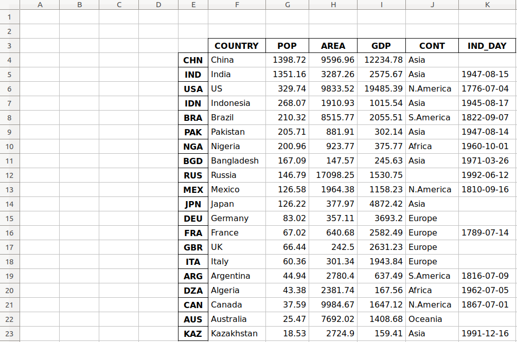
As you can see, the table starts in the third row 2 and the fifth column E.
.read_excel() also has the optional parameter sheet_name that specifies which worksheets to read when loading data. It can take on one of the following values:
- The zero-based index of the worksheet
- The name of the worksheet
- The list of indices or names to read multiple sheets
- The value
Noneto read all sheets
Here’s how you would use this parameter in your code:
>>>
>>> df = pd.read_excel('data.xlsx', sheet_name=0, index_col=0,
...                    parse_dates=['IND_DAY'])
>>> df = pd.read_excel('data.xlsx', sheet_name='COUNTRIES', index_col=0,
...                    parse_dates=['IND_DAY'])
Both statements above create the same DataFrame because the sheet_name parameters have the same values. In both cases, sheet_name=0 and sheet_name='COUNTRIES' refer to the same worksheet. The argument parse_dates=['IND_DAY'] tells pandas to try to consider the values in this column as dates or times.
There are other optional parameters you can use with .read_excel() and .to_excel() to determine the Excel engine, the encoding, the way to handle missing values and infinities, the method for writing column names and row labels, and so on.
SQL Files
pandas IO tools can also read and write databases. In this next example, you’ll write your data to a database called data.db. To get started, you’ll need the SQLAlchemy package. To learn more about it, you can read the official ORM tutorial. You’ll also need the database driver. Python has a built-in driver for SQLite.
You can install SQLAlchemy with pip:
You can also install it with Conda:
$ conda install sqlalchemy
Once you have SQLAlchemy installed, import create_engine() and create a database engine:
>>>
>>> from sqlalchemy import create_engine
>>> engine = create_engine('sqlite:///data.db', echo=False)
Now that you have everything set up, the next step is to create a DataFrame object. It’s convenient to specify the data types and apply .to_sql().
>>>
>>> dtypes = {'POP': 'float64', 'AREA': 'float64', 'GDP': 'float64',
...           'IND_DAY': 'datetime64'}
>>> df = pd.DataFrame(data=data).T.astype(dtype=dtypes)
>>> df.dtypes
COUNTRY            object
POP               float64
AREA              float64
GDP               float64
CONT               object
IND_DAY    datetime64[ns]
dtype: object
.astype() is a very convenient method you can use to set multiple data types at once.
Once you’ve created your DataFrame, you can save it to the database with .to_sql():
>>>
>>> df.to_sql('data.db', con=engine, index_label='ID')
The parameter con is used to specify the database connection or engine that you want to use. The optional parameter index_label specifies how to call the database column with the row labels. You’ll often see it take on the value ID, Id, or id.
You should get the database data.db with a single table that looks like this:
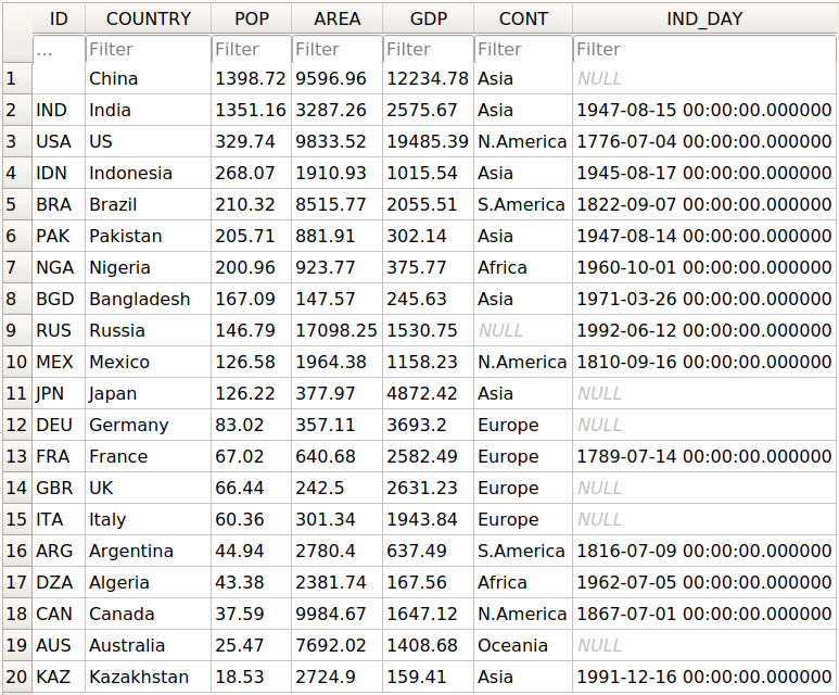
The first column contains the row labels. To omit writing them into the database, pass index=False to .to_sql(). The other columns correspond to the columns of the DataFrame.
There are a few more optional parameters. For example, you can use schema to specify the database schema and dtype to determine the types of the database columns. You can also use if_exists, which says what to do if a database with the same name and path already exists:
if_exists='fail'raises a ValueError and is the default.if_exists='replace'drops the table and inserts new values.if_exists='append'inserts new values into the table.
You can load the data from the database with read_sql():
>>>
>>> df = pd.read_sql('data.db', con=engine, index_col='ID')
>>> df
        COUNTRY      POP      AREA       GDP       CONT    IND_DAY
ID
CHN       China  1398.72   9596.96  12234.78       Asia        NaT
IND       India  1351.16   3287.26   2575.67       Asia 1947-08-15
USA          US   329.74   9833.52  19485.39  N.America 1776-07-04
IDN   Indonesia   268.07   1910.93   1015.54       Asia 1945-08-17
BRA      Brazil   210.32   8515.77   2055.51  S.America 1822-09-07
PAK    Pakistan   205.71    881.91    302.14       Asia 1947-08-14
NGA     Nigeria   200.96    923.77    375.77     Africa 1960-10-01
BGD  Bangladesh   167.09    147.57    245.63       Asia 1971-03-26
RUS      Russia   146.79  17098.25   1530.75       None 1992-06-12
MEX      Mexico   126.58   1964.38   1158.23  N.America 1810-09-16
JPN       Japan   126.22    377.97   4872.42       Asia        NaT
DEU     Germany    83.02    357.11   3693.20     Europe        NaT
FRA      France    67.02    640.68   2582.49     Europe 1789-07-14
GBR          UK    66.44    242.50   2631.23     Europe        NaT
ITA       Italy    60.36    301.34   1943.84     Europe        NaT
ARG   Argentina    44.94   2780.40    637.49  S.America 1816-07-09
DZA     Algeria    43.38   2381.74    167.56     Africa 1962-07-05
CAN      Canada    37.59   9984.67   1647.12  N.America 1867-07-01
AUS   Australia    25.47   7692.02   1408.68    Oceania        NaT
KAZ  Kazakhstan    18.53   2724.90    159.41       Asia 1991-12-16
The parameter index_col specifies the name of the column with the row labels. Note that this inserts an extra row after the header that starts with ID. You can fix this behavior with the following line of code:
>>>
>>> df.index.name = None
>>> df
        COUNTRY      POP      AREA       GDP       CONT    IND_DAY
CHN       China  1398.72   9596.96  12234.78       Asia        NaT
IND       India  1351.16   3287.26   2575.67       Asia 1947-08-15
USA          US   329.74   9833.52  19485.39  N.America 1776-07-04
IDN   Indonesia   268.07   1910.93   1015.54       Asia 1945-08-17
BRA      Brazil   210.32   8515.77   2055.51  S.America 1822-09-07
PAK    Pakistan   205.71    881.91    302.14       Asia 1947-08-14
NGA     Nigeria   200.96    923.77    375.77     Africa 1960-10-01
BGD  Bangladesh   167.09    147.57    245.63       Asia 1971-03-26
RUS      Russia   146.79  17098.25   1530.75       None 1992-06-12
MEX      Mexico   126.58   1964.38   1158.23  N.America 1810-09-16
JPN       Japan   126.22    377.97   4872.42       Asia        NaT
DEU     Germany    83.02    357.11   3693.20     Europe        NaT
FRA      France    67.02    640.68   2582.49     Europe 1789-07-14
GBR          UK    66.44    242.50   2631.23     Europe        NaT
ITA       Italy    60.36    301.34   1943.84     Europe        NaT
ARG   Argentina    44.94   2780.40    637.49  S.America 1816-07-09
DZA     Algeria    43.38   2381.74    167.56     Africa 1962-07-05
CAN      Canada    37.59   9984.67   1647.12  N.America 1867-07-01
AUS   Australia    25.47   7692.02   1408.68    Oceania        NaT
KAZ  Kazakhstan    18.53   2724.90    159.41       Asia 1991-12-16
Now you have the same DataFrame object as before.
Note that the continent for Russia is now None instead of nan. If you want to fill the missing values with nan, then you can use .fillna():
>>>
>>> df.fillna(value=float('nan'), inplace=True)
.fillna() replaces all missing values with whatever you pass to value. Here, you passed float('nan'), which says to fill all missing values with nan.
Also note that you didn’t have to pass parse_dates=['IND_DAY'] to read_sql(). That’s because your database was able to detect that the last column contains dates. However, you can pass parse_dates if you’d like. You’ll get the same results.
There are other functions that you can use to read databases, like read_sql_table() and read_sql_query(). Feel free to try them out!
Pickle Files
Pickling is the act of converting Python objects into byte streams. Unpickling is the inverse process. Python pickle files are the binary files that keep the data and hierarchy of Python objects. They usually have the extension .pickle or .pkl.
You can save your DataFrame in a pickle file with .to_pickle():
>>>
>>> dtypes = {'POP': 'float64', 'AREA': 'float64', 'GDP': 'float64',
...           'IND_DAY': 'datetime64'}
>>> df = pd.DataFrame(data=data).T.astype(dtype=dtypes)
>>> df.to_pickle('data.pickle')
Like you did with databases, it can be convenient first to specify the data types. Then, you create a file data.pickle to contain your data. You could also pass an integer value to the optional parameter protocol, which specifies the protocol of the pickler.
You can get the data from a pickle file with read_pickle():
>>>
>>> df = pd.read_pickle('data.pickle')
>>> df
        COUNTRY      POP      AREA       GDP       CONT    IND_DAY
CHN       China  1398.72   9596.96  12234.78       Asia        NaT
IND       India  1351.16   3287.26   2575.67       Asia 1947-08-15
USA          US   329.74   9833.52  19485.39  N.America 1776-07-04
IDN   Indonesia   268.07   1910.93   1015.54       Asia 1945-08-17
BRA      Brazil   210.32   8515.77   2055.51  S.America 1822-09-07
PAK    Pakistan   205.71    881.91    302.14       Asia 1947-08-14
NGA     Nigeria   200.96    923.77    375.77     Africa 1960-10-01
BGD  Bangladesh   167.09    147.57    245.63       Asia 1971-03-26
RUS      Russia   146.79  17098.25   1530.75        NaN 1992-06-12
MEX      Mexico   126.58   1964.38   1158.23  N.America 1810-09-16
JPN       Japan   126.22    377.97   4872.42       Asia        NaT
DEU     Germany    83.02    357.11   3693.20     Europe        NaT
FRA      France    67.02    640.68   2582.49     Europe 1789-07-14
GBR          UK    66.44    242.50   2631.23     Europe        NaT
ITA       Italy    60.36    301.34   1943.84     Europe        NaT
ARG   Argentina    44.94   2780.40    637.49  S.America 1816-07-09
DZA     Algeria    43.38   2381.74    167.56     Africa 1962-07-05
CAN      Canada    37.59   9984.67   1647.12  N.America 1867-07-01
AUS   Australia    25.47   7692.02   1408.68    Oceania        NaT
KAZ  Kazakhstan    18.53   2724.90    159.41       Asia 1991-12-16
read_pickle() returns the DataFrame with the stored data. You can also check the data types:
>>>
>>> df.dtypes
COUNTRY            object
POP               float64
AREA              float64
GDP               float64
CONT               object
IND_DAY    datetime64[ns]
dtype: object
These are the same ones that you specified before using .to_pickle().
As a word of caution, you should always beware of loading pickles from untrusted sources. This can be dangerous! When you unpickle an untrustworthy file, it could execute arbitrary code on your machine, gain remote access to your computer, or otherwise exploit your device in other ways.
Working With Big Data
If your files are too large for saving or processing, then there are several approaches you can take to reduce the required disk space:
- Compress your files
- Choose only the columns you want
- Omit the rows you don’t need
- Force the use of less precise data types
- Split the data into chunks
You’ll take a look at each of these techniques in turn.
Compress and Decompress Files
You can create an archive file like you would a regular one, with the addition of a suffix that corresponds to the desired compression type:
'.gz''.bz2''.zip''.xz'
pandas can deduce the compression type by itself:
>>>
>>> df = pd.DataFrame(data=data).T
>>> df.to_csv('data.csv.zip')
Here, you create a compressed .csv file as an archive. The size of the regular .csv file is 1048 bytes, while the compressed file only has 766 bytes.
You can open this compressed file as usual with the pandas read_csv() function:
>>>
>>> df = pd.read_csv('data.csv.zip', index_col=0,
...                  parse_dates=['IND_DAY'])
>>> df
        COUNTRY      POP      AREA       GDP       CONT    IND_DAY
CHN       China  1398.72   9596.96  12234.78       Asia        NaT
IND       India  1351.16   3287.26   2575.67       Asia 1947-08-15
USA          US   329.74   9833.52  19485.39  N.America 1776-07-04
IDN   Indonesia   268.07   1910.93   1015.54       Asia 1945-08-17
BRA      Brazil   210.32   8515.77   2055.51  S.America 1822-09-07
PAK    Pakistan   205.71    881.91    302.14       Asia 1947-08-14
NGA     Nigeria   200.96    923.77    375.77     Africa 1960-10-01
BGD  Bangladesh   167.09    147.57    245.63       Asia 1971-03-26
RUS      Russia   146.79  17098.25   1530.75        NaN 1992-06-12
MEX      Mexico   126.58   1964.38   1158.23  N.America 1810-09-16
JPN       Japan   126.22    377.97   4872.42       Asia        NaT
DEU     Germany    83.02    357.11   3693.20     Europe        NaT
FRA      France    67.02    640.68   2582.49     Europe 1789-07-14
GBR          UK    66.44    242.50   2631.23     Europe        NaT
ITA       Italy    60.36    301.34   1943.84     Europe        NaT
ARG   Argentina    44.94   2780.40    637.49  S.America 1816-07-09
DZA     Algeria    43.38   2381.74    167.56     Africa 1962-07-05
CAN      Canada    37.59   9984.67   1647.12  N.America 1867-07-01
AUS   Australia    25.47   7692.02   1408.68    Oceania        NaT
KAZ  Kazakhstan    18.53   2724.90    159.41       Asia 1991-12-16
read_csv() decompresses the file before reading it into a DataFrame.
You can specify the type of compression with the optional parameter compression, which can take on any of the following values:
'infer''gzip''bz2''zip''xz'None
The default value compression='infer' indicates that pandas should deduce the compression type from the file extension.
Here’s how you would compress a pickle file:
>>>
>>> df = pd.DataFrame(data=data).T
>>> df.to_pickle('data.pickle.compress', compression='gzip')
You should get the file data.pickle.compress that you can later decompress and read:
>>>
>>> df = pd.read_pickle('data.pickle.compress', compression='gzip')
df again corresponds to the DataFrame with the same data as before.
You can give the other compression methods a try, as well. If you’re using pickle files, then keep in mind that the .zip format supports reading only.
Choose Columns
The pandas read_csv() and read_excel() functions have the optional parameter usecols that you can use to specify the columns you want to load from the file. You can pass the list of column names as the corresponding argument:
>>>
>>> df = pd.read_csv('data.csv', usecols=['COUNTRY', 'AREA'])
>>> df
       COUNTRY      AREA
0        China   9596.96
1        India   3287.26
2           US   9833.52
3    Indonesia   1910.93
4       Brazil   8515.77
5     Pakistan    881.91
6      Nigeria    923.77
7   Bangladesh    147.57
8       Russia  17098.25
9       Mexico   1964.38
10       Japan    377.97
11     Germany    357.11
12      France    640.68
13          UK    242.50
14       Italy    301.34
15   Argentina   2780.40
16     Algeria   2381.74
17      Canada   9984.67
18   Australia   7692.02
19  Kazakhstan   2724.90
Now you have a DataFrame that contains less data than before. Here, there are only the names of the countries and their areas.
Instead of the column names, you can also pass their indices:
>>>
>>> df = pd.read_csv('data.csv',index_col=0, usecols=[0, 1, 3])
>>> df
        COUNTRY      AREA
CHN       China   9596.96
IND       India   3287.26
USA          US   9833.52
IDN   Indonesia   1910.93
BRA      Brazil   8515.77
PAK    Pakistan    881.91
NGA     Nigeria    923.77
BGD  Bangladesh    147.57
RUS      Russia  17098.25
MEX      Mexico   1964.38
JPN       Japan    377.97
DEU     Germany    357.11
FRA      France    640.68
GBR          UK    242.50
ITA       Italy    301.34
ARG   Argentina   2780.40
DZA     Algeria   2381.74
CAN      Canada   9984.67
AUS   Australia   7692.02
KAZ  Kazakhstan   2724.90
Expand the code block below to compare these results with the file 'data.csv':
,COUNTRY,POP,AREA,GDP,CONT,IND_DAY
CHN,China,1398.72,9596.96,12234.78,Asia,
IND,India,1351.16,3287.26,2575.67,Asia,1947-08-15
USA,US,329.74,9833.52,19485.39,N.America,1776-07-04
IDN,Indonesia,268.07,1910.93,1015.54,Asia,1945-08-17
BRA,Brazil,210.32,8515.77,2055.51,S.America,1822-09-07
PAK,Pakistan,205.71,881.91,302.14,Asia,1947-08-14
NGA,Nigeria,200.96,923.77,375.77,Africa,1960-10-01
BGD,Bangladesh,167.09,147.57,245.63,Asia,1971-03-26
RUS,Russia,146.79,17098.25,1530.75,,1992-06-12
MEX,Mexico,126.58,1964.38,1158.23,N.America,1810-09-16
JPN,Japan,126.22,377.97,4872.42,Asia,
DEU,Germany,83.02,357.11,3693.2,Europe,
FRA,France,67.02,640.68,2582.49,Europe,1789-07-14
GBR,UK,66.44,242.5,2631.23,Europe,
ITA,Italy,60.36,301.34,1943.84,Europe,
ARG,Argentina,44.94,2780.4,637.49,S.America,1816-07-09
DZA,Algeria,43.38,2381.74,167.56,Africa,1962-07-05
CAN,Canada,37.59,9984.67,1647.12,N.America,1867-07-01
AUS,Australia,25.47,7692.02,1408.68,Oceania,
KAZ,Kazakhstan,18.53,2724.9,159.41,Asia,1991-12-16
You can see the following columns:
- The column at index
0contains the row labels. - The column at index
1contains the country names. - The column at index
3contains the areas.
Simlarly, read_sql() has the optional parameter columns that takes a list of column names to read:
>>>
>>> df = pd.read_sql('data.db', con=engine, index_col='ID',
...                  columns=['COUNTRY', 'AREA'])
>>> df.index.name = None
>>> df
        COUNTRY      AREA
CHN       China   9596.96
IND       India   3287.26
USA          US   9833.52
IDN   Indonesia   1910.93
BRA      Brazil   8515.77
PAK    Pakistan    881.91
NGA     Nigeria    923.77
BGD  Bangladesh    147.57
RUS      Russia  17098.25
MEX      Mexico   1964.38
JPN       Japan    377.97
DEU     Germany    357.11
FRA      France    640.68
GBR          UK    242.50
ITA       Italy    301.34
ARG   Argentina   2780.40
DZA     Algeria   2381.74
CAN      Canada   9984.67
AUS   Australia   7692.02
KAZ  Kazakhstan   2724.90
Again, the DataFrame only contains the columns with the names of the countries and areas. If columns is None or omitted, then all of the columns will be read, as you saw before. The default behavior is columns=None.
Omit Rows
When you test an algorithm for data processing or machine learning, you often don’t need the entire dataset. It’s convenient to load only a subset of the data to speed up the process. The pandas read_csv() and read_excel() functions have some optional parameters that allow you to select which rows you want to load:
skiprows: either the number of rows to skip at the beginning of the file if it’s an integer, or the zero-based indices of the rows to skip if it’s a list-like objectskipfooter: the number of rows to skip at the end of the filenrows: the number of rows to read
Here’s how you would skip rows with odd zero-based indices, keeping the even ones:
>>>
>>> df = pd.read_csv('data.csv', index_col=0, skiprows=range(1, 20, 2))
>>> df
        COUNTRY      POP     AREA      GDP       CONT     IND_DAY
IND       India  1351.16  3287.26  2575.67       Asia  1947-08-15
IDN   Indonesia   268.07  1910.93  1015.54       Asia  1945-08-17
PAK    Pakistan   205.71   881.91   302.14       Asia  1947-08-14
BGD  Bangladesh   167.09   147.57   245.63       Asia  1971-03-26
MEX      Mexico   126.58  1964.38  1158.23  N.America  1810-09-16
DEU     Germany    83.02   357.11  3693.20     Europe         NaN
GBR          UK    66.44   242.50  2631.23     Europe         NaN
ARG   Argentina    44.94  2780.40   637.49  S.America  1816-07-09
CAN      Canada    37.59  9984.67  1647.12  N.America  1867-07-01
KAZ  Kazakhstan    18.53  2724.90   159.41       Asia  1991-12-16
In this example, skiprows is range(1, 20, 2) and corresponds to the values 1, 3, …, 19. The instances of the Python built-in class range behave like sequences. The first row of the file data.csv is the header row. It has the index 0, so pandas loads it in. The second row with index 1 corresponds to the label CHN, and pandas skips it. The third row with the index 2 and label IND is loaded, and so on.
If you want to choose rows randomly, then skiprows can be a list or NumPy array with pseudo-random numbers, obtained either with pure Python or with NumPy.
Force Less Precise Data Types
If you’re okay with less precise data types, then you can potentially save a significant amount of memory! First, get the data types with .dtypes again:
>>>
>>> df = pd.read_csv('data.csv', index_col=0, parse_dates=['IND_DAY'])
>>> df.dtypes
COUNTRY            object
POP               float64
AREA              float64
GDP               float64
CONT               object
IND_DAY    datetime64[ns]
dtype: object
The columns with the floating-point numbers are 64-bit floats. Each number of this type float64 consumes 64 bits or 8 bytes. Each column has 20 numbers and requires 160 bytes. You can verify this with .memory_usage():
>>>
>>> df.memory_usage()
Index      160
COUNTRY    160
POP        160
AREA       160
GDP        160
CONT       160
IND_DAY    160
dtype: int64
.memory_usage() returns an instance of Series with the memory usage of each column in bytes. You can conveniently combine it with .loc[] and .sum() to get the memory for a group of columns:
>>>
>>> df.loc[:, ['POP', 'AREA', 'GDP']].memory_usage(index=False).sum()
480
This example shows how you can combine the numeric columns 'POP', 'AREA', and 'GDP' to get their total memory requirement. The argument index=False excludes data for row labels from the resulting Series object. For these three columns, you’ll need 480 bytes.
You can also extract the data values in the form of a NumPy array with .to_numpy() or .values. Then, use the .nbytes attribute to get the total bytes consumed by the items of the array:
>>>
>>> df.loc[:, ['POP', 'AREA', 'GDP']].to_numpy().nbytes
480
The result is the same 480 bytes. So, how do you save memory?
In this case, you can specify that your numeric columns 'POP', 'AREA', and 'GDP' should have the type float32. Use the optional parameter dtype to do this:
>>>
>>> dtypes = {'POP': 'float32', 'AREA': 'float32', 'GDP': 'float32'}
>>> df = pd.read_csv('data.csv', index_col=0, dtype=dtypes,
...                  parse_dates=['IND_DAY'])
The dictionary dtypes specifies the desired data types for each column. It’s passed to the pandas read_csv() function as the argument that corresponds to the parameter dtype.
Now you can verify that each numeric column needs 80 bytes, or 4 bytes per item:
>>>
>>> df.dtypes
COUNTRY            object
POP               float32
AREA              float32
GDP               float32
CONT               object
IND_DAY    datetime64[ns]
dtype: object
>>> df.memory_usage()
Index      160
COUNTRY    160
POP         80
AREA        80
GDP         80
CONT       160
IND_DAY    160
dtype: int64
>>> df.loc[:, ['POP', 'AREA', 'GDP']].memory_usage(index=False).sum()
240
>>> df.loc[:, ['POP', 'AREA', 'GDP']].to_numpy().nbytes
240
Each value is a floating-point number of 32 bits or 4 bytes. The three numeric columns contain 20 items each. In total, you’ll need 240 bytes of memory when you work with the type float32. This is half the size of the 480 bytes you’d need to work with float64.
In addition to saving memory, you can significantly reduce the time required to process data by using float32 instead of float64 in some cases.
Use Chunks to Iterate Through Files
Another way to deal with very large datasets is to split the data into smaller chunks and process one chunk at a time. If you use read_csv(), read_json() or read_sql(), then you can specify the optional parameter chunksize:
>>>
>>> data_chunk = pd.read_csv('data.csv', index_col=0, chunksize=8)
>>> type(data_chunk)
<class 'pandas.io.parsers.TextFileReader'>
>>> hasattr(data_chunk, '__iter__')
True
>>> hasattr(data_chunk, '__next__')
True
chunksize defaults to None and can take on an integer value that indicates the number of items in a single chunk. When chunksize is an integer, read_csv() returns an iterable that you can use in a for loop to get and process only a fragment of the dataset in each iteration:
>>>
>>> for df_chunk in pd.read_csv('data.csv', index_col=0, chunksize=8):
...     print(df_chunk, end='nn')
...     print('memory:', df_chunk.memory_usage().sum(), 'bytes',
...           end='nnn')
...
        COUNTRY      POP     AREA       GDP       CONT     IND_DAY
CHN       China  1398.72  9596.96  12234.78       Asia         NaN
IND       India  1351.16  3287.26   2575.67       Asia  1947-08-15
USA          US   329.74  9833.52  19485.39  N.America  1776-07-04
IDN   Indonesia   268.07  1910.93   1015.54       Asia  1945-08-17
BRA      Brazil   210.32  8515.77   2055.51  S.America  1822-09-07
PAK    Pakistan   205.71   881.91    302.14       Asia  1947-08-14
NGA     Nigeria   200.96   923.77    375.77     Africa  1960-10-01
BGD  Bangladesh   167.09   147.57    245.63       Asia  1971-03-26

memory: 448 bytes


       COUNTRY     POP      AREA      GDP       CONT     IND_DAY
RUS     Russia  146.79  17098.25  1530.75        NaN  1992-06-12
MEX     Mexico  126.58   1964.38  1158.23  N.America  1810-09-16
JPN      Japan  126.22    377.97  4872.42       Asia         NaN
DEU    Germany   83.02    357.11  3693.20     Europe         NaN
FRA     France   67.02    640.68  2582.49     Europe  1789-07-14
GBR         UK   66.44    242.50  2631.23     Europe         NaN
ITA      Italy   60.36    301.34  1943.84     Europe         NaN
ARG  Argentina   44.94   2780.40   637.49  S.America  1816-07-09

memory: 448 bytes


        COUNTRY    POP     AREA      GDP       CONT     IND_DAY
DZA     Algeria  43.38  2381.74   167.56     Africa  1962-07-05
CAN      Canada  37.59  9984.67  1647.12  N.America  1867-07-01
AUS   Australia  25.47  7692.02  1408.68    Oceania         NaN
KAZ  Kazakhstan  18.53  2724.90   159.41       Asia  1991-12-16

memory: 224 bytes
In this example, the chunksize is 8. The first iteration of the for loop returns a DataFrame with the first eight rows of the dataset only. The second iteration returns another DataFrame with the next eight rows. The third and last iteration returns the remaining four rows.
In each iteration, you get and process the DataFrame with the number of rows equal to chunksize. It’s possible to have fewer rows than the value of chunksize in the last iteration. You can use this functionality to control the amount of memory required to process data and keep that amount reasonably small.
Conclusion
You now know how to save the data and labels from pandas DataFrame objects to different kinds of files. You also know how to load your data from files and create DataFrame objects.
You’ve used the pandas read_csv() and .to_csv() methods to read and write CSV files. You also used similar methods to read and write Excel, JSON, HTML, SQL, and pickle files. These functions are very convenient and widely used. They allow you to save or load your data in a single function or method call.
You’ve also learned how to save time, memory, and disk space when working with large data files:
- Compress or decompress files
- Choose the rows and columns you want to load
- Use less precise data types
- Split data into chunks and process them one by one
You’ve mastered a significant step in the machine learning and data science process! If you have any questions or comments, then please put them in the comments section below.
Watch Now This tutorial has a related video course created by the Real Python team. Watch it together with the written tutorial to deepen your understanding: Reading and Writing Files With Pandas
Время на прочтение
5 мин
Количество просмотров 63K
Excel — это чрезвычайно распространённый инструмент для анализа данных. С ним легко научиться работать, есть он практически на каждом компьютере, а тот, кто его освоил, может с его помощью решать довольно сложные задачи. Python часто считают инструментом, возможности которого практически безграничны, но который освоить сложнее, чем Excel. Автор материала, перевод которого мы сегодня публикуем, хочет рассказать о решении с помощью Python трёх задач, которые обычно решают в Excel. Эта статья представляет собой нечто вроде введения в Python для тех, кто хорошо знает Excel.

Загрузка данных
Начнём с импорта Python-библиотеки pandas и с загрузки в датафреймы данных, которые хранятся на листах sales и states книги Excel. Такие же имена мы дадим и соответствующим датафреймам.
import pandas as pd
sales = pd.read_excel('https://github.com/datagy/mediumdata/raw/master/pythonexcel.xlsx', sheet_name = 'sales')
states = pd.read_excel('https://github.com/datagy/mediumdata/raw/master/pythonexcel.xlsx', sheet_name = 'states')
Теперь воспользуемся методом .head() датафрейма sales для того чтобы вывести элементы, находящиеся в начале датафрейма:
print(sales.head())
Сравним то, что будет выведено, с тем, что можно видеть в Excel.
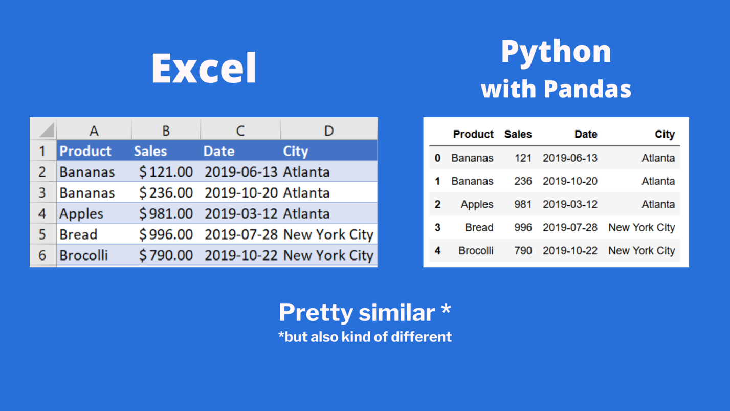
Сравнение внешнего вида данных, выводимых в Excel, с внешним видом данных, выводимых из датафрейма pandas
Тут можно видеть, что результаты визуализации данных из датафрейма очень похожи на то, что можно видеть в Excel. Но тут имеются и некоторые очень важные различия:
- Нумерация строк в Excel начинается с 1, а в pandas номер (индекс) первой строки равняется 0.
- В Excel столбцы имеют буквенные обозначения, начинающиеся с буквы
A, а в pandas названия столбцов соответствуют именам соответствующих переменных.
Продолжим исследование возможностей pandas, позволяющих решать задачи, которые обычно решают в Excel.
Реализация возможностей Excel-функции IF в Python
В Excel существует очень удобная функция IF, которая позволяет, например, записать что-либо в ячейку, основываясь на проверке того, что находится в другой ячейке. Предположим, нужно создать в Excel новый столбец, ячейки которого будут сообщать нам о том, превышают ли 500 значения, записанные в соответствующие ячейки столбца B. В Excel такому столбцу (в нашем случае это столбец E) можно назначить заголовок MoreThan500, записав соответствующий текст в ячейку E1. После этого, в ячейке E2, можно ввести следующее:
=IF([@Sales]>500, "Yes", "No")
Использование функции IF в Excel
Для того чтобы сделать то же самое с использованием pandas, можно воспользоваться списковым включением (list comprehension):
sales['MoreThan500'] = ['Yes' if x > 500 else 'No' for x in sales['Sales']]
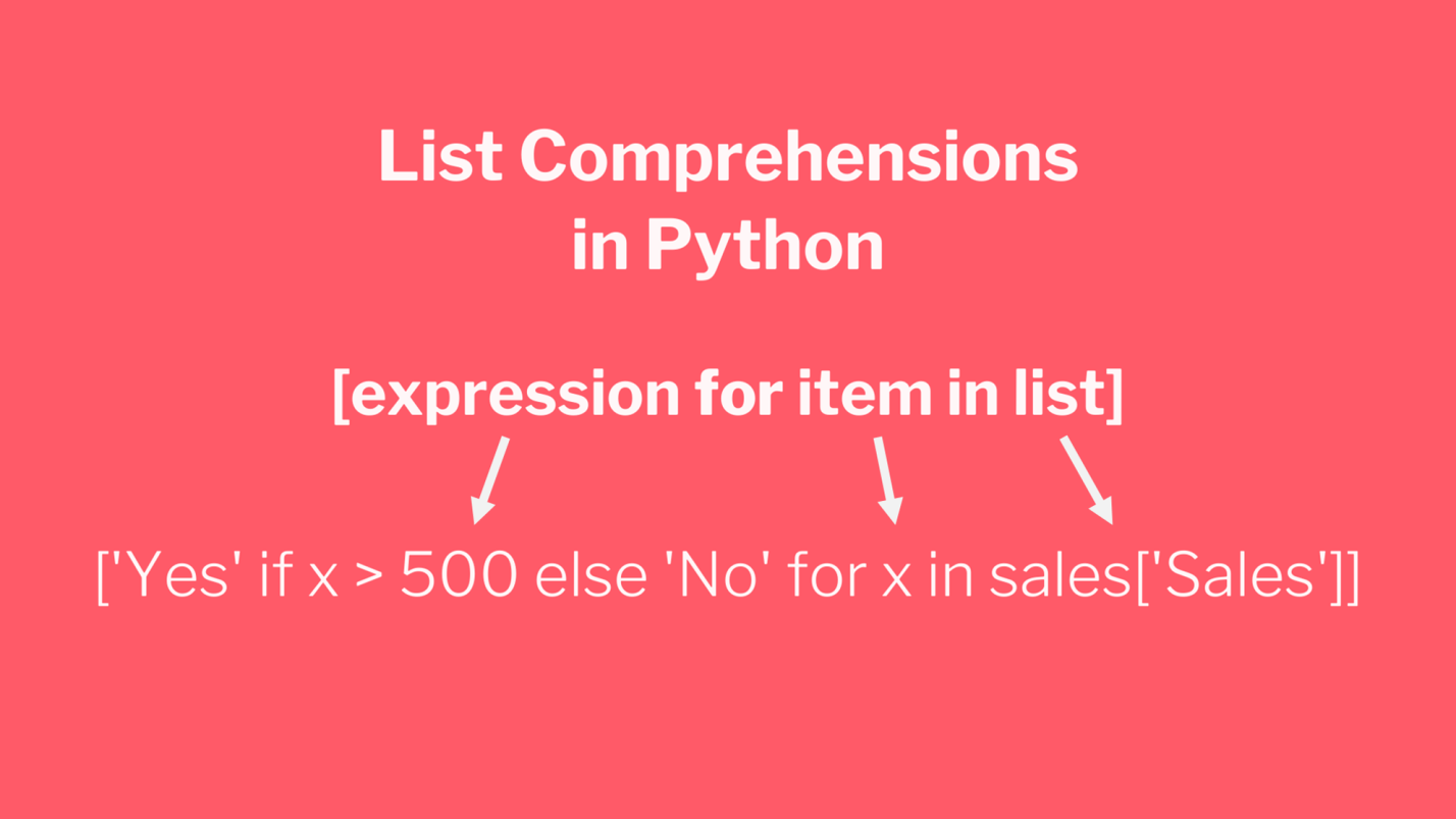
Списковые включения в Python: если текущее значение больше 500 — в список попадает Yes, в противном случае — No
Списковые включения — это отличное средство для решения подобных задач, позволяющее упростить код за счёт уменьшения потребности в сложных конструкциях вида if/else. Ту же задачу можно решить и с помощью if/else, но предложенный подход экономит время и делает код немного чище. Подробности о списковых включениях можно найти здесь.
Реализация возможностей Excel-функции VLOOKUP в Python
В нашем наборе данных, на одном из листов Excel, есть названия городов, а на другом — названия штатов и провинций. Как узнать о том, где именно находится каждый город? Для этого подходит Excel-функция VLOOKUP, с помощью которой можно связать данные двух таблиц. Эта функция работает по принципу левого соединения, когда сохраняется каждая запись из набора данных, находящегося в левой части выражения. Применяя функцию VLOOKUP, мы предлагаем системе выполнить поиск определённого значения в заданном столбце указанного листа, а затем — вернуть значение, которое находится на заданное число столбцов правее найденного значения. Вот как это выглядит:
=VLOOKUP([@City],states,2,false)
Зададим на листе sales заголовок столбца F как State и воспользуемся функцией VLOOKUP для того чтобы заполнить ячейки этого столбца названиями штатов и провинций, в которых расположены города.

Использование функции VLOOKUP в Excel
В Python сделать то же самое можно, воспользовавшись методом merge из pandas. Он принимает два датафрейма и объединяет их. Для решения этой задачи нам понадобится следующий код:
sales = pd.merge(sales, states, how='left', on='City')
Разберём его:
- Первый аргумент метода
merge— это исходный датафрейм. - Второй аргумент — это датафрейм, в котором мы ищем значения.
- Аргумент
howуказывает на то, как именно мы хотим соединить данные. - Аргумент
onуказывает на переменную, по которой нужно выполнить соединение (тут ещё можно использовать аргументыleft_onиright_on, нужные в том случае, если интересующие нас данные в разных датафреймах названы по-разному).
Сводные таблицы
Сводные таблицы (Pivot Tables) — это одна из самых мощных возможностей Excel. Такие таблицы позволяют очень быстро извлекать ценные сведения из больших наборов данных. Создадим в Excel сводную таблицу, выводящую сведения о суммарных продажах по каждому городу.
Создание сводной таблицы в Excel
Как видите, для создания подобной таблицы достаточно перетащить поле City в раздел Rows, а поле Sales — в раздел Values. После этого Excel автоматически выведет суммарные продажи для каждого города.
Для того чтобы создать такую же сводную таблицу в pandas, нужно будет написать следующий код:
sales.pivot_table(index = 'City', values = 'Sales', aggfunc = 'sum')
Разберём его:
- Здесь мы используем метод
sales.pivot_table, сообщая pandas о том, что мы хотим создать сводную таблицу, основанную на датафреймеsales. - Аргумент
indexуказывает на столбец, по которому мы хотим агрегировать данные. - Аргумент
valuesуказывает на то, какие значения мы собираемся агрегировать. - Аргумент
aggfuncзадаёт функцию, которую мы хотим использовать при обработке значений (тут ещё можно воспользоваться функциямиmean,max,minи так далее).
Итоги
Из этого материала вы узнали о том, как импортировать Excel-данные в pandas, о том, как реализовать средствами Python и pandas возможности Excel-функций IF и VLOOKUP, а также о том, как воспроизвести средствами pandas функционал сводных таблиц Excel. Возможно, сейчас вы задаётесь вопросом о том, зачем вам пользоваться pandas, если то же самое можно сделать и в Excel. На этот вопрос нет однозначного ответа. Python позволяет создавать код, который поддаётся тонкой настройке и глубокому исследованию. Такой код можно использовать многократно. Средствами Python можно описывать очень сложные схемы анализа данных. А возможностей Excel, вероятно, достаточно лишь для менее масштабных исследований данных. Если вы до этого момента пользовались только Excel — рекомендую испытать Python и pandas, и узнать о том, что у вас из этого получится.
А какие инструменты вы используете для анализа данных?
Напоминаем, что у нас продолжается конкурс прогнозов, в котором можно выиграть новенький iPhone. Еще есть время ворваться в него, и сделать максимально точный прогноз по злободневным величинам.

Excel sheets are very instinctive and user-friendly, which makes them ideal for manipulating large datasets even for less technical folks. If you are looking for places to learn to manipulate and automate stuff in excel files using Python, look no more. You are at the right place.
Python Pandas With Excel Sheet
In this article, you will learn how to use Pandas to work with Excel spreadsheets. At the end of the article, you will have the knowledge of:
- Necessary modules are needed for this and how to set them up in your system.
- Reading data from excel files into pandas using Python.
- Exploring the data from excel files in Pandas.
- Using functions to manipulate and reshape the data in Pandas.
Installation
To install Pandas in Anaconda, we can use the following command in Anaconda Terminal:
conda install pandas
To install Pandas in regular Python (Non-Anaconda), we can use the following command in the command prompt:
pip install pandas
Getting Started
First of all, we need to import the Pandas module which can be done by running the command: Pandas
Python3
Input File: Let’s suppose the excel file looks like this
Sheet 1:
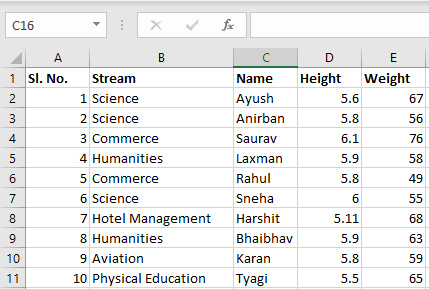
Sheet 2:
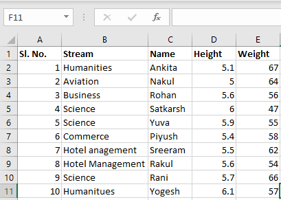
Now we can import the excel file using the read_excel function in Pandas. The second statement reads the data from excel and stores it into a pandas Data Frame which is represented by the variable newData. If there are multiple sheets in the excel workbook, the command will import data of the first sheet. To make a data frame with all the sheets in the workbook, the easiest method is to create different data frames separately and then concatenate them. The read_excel method takes argument sheet_name and index_col where we can specify the sheet of which the data frame should be made of and index_col specifies the title column, as is shown below:
Python3
file =('path_of_excel_file')
newData = pds.read_excel(file)
newData
Output:
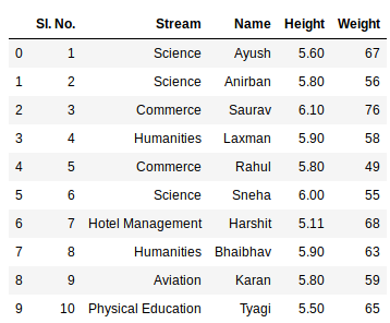
Example:
The third statement concatenates both sheets. Now to check the whole data frame, we can simply run the following command:
Python3
sheet1 = pds.read_excel(file,
sheet_name = 0,
index_col = 0)
sheet2 = pds.read_excel(file,
sheet_name = 1,
index_col = 0)
newData = pds.concat([sheet1, sheet2])
newData
Output:
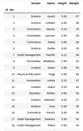
To view 5 columns from the top and from the bottom of the data frame, we can run the command. This head() and tail() method also take arguments as numbers for the number of columns to show.
Python3
newData.head()
newData.tail()
Output:
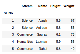
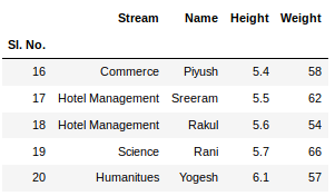
The shape() method can be used to view the number of rows and columns in the data frame as follows:
Python3
Output:

If any column contains numerical data, we can sort that column using the sort_values() method in pandas as follows:
Python3
sorted_column = newData.sort_values(['Height'], ascending = False)
Now, let’s suppose we want the top 5 values of the sorted column, we can use the head() method here:
Python3
sorted_column['Height'].head(5)
Output:
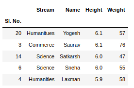
We can do that with any numerical column of the data frame as shown below:
Python3
Output:
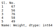
Now, suppose our data is mostly numerical. We can get the statistical information like mean, max, min, etc. about the data frame using the describe() method as shown below:
Python3
Output:
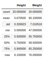
This can also be done separately for all the numerical columns using the following command:
Python3
Output:

Other statistical information can also be calculated using the respective methods. Like in excel, formulas can also be applied and calculated columns can be created as follows:
Python3
newData['calculated_column'] =
newData[“Height”] + newData[“Weight”]
newData['calculated_column'].head()
Output:
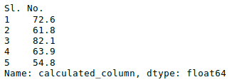
After operating on the data in the data frame, we can export the data back to an excel file using the method to_excel. For this we need to specify an output excel file where the transformed data is to be written, as shown below:
Python3
newData.to_excel('Output File.xlsx')
Output: