
We have two options to refer a cell in excel VBA Absolute references and Relative references. Default Excel records macro in Absolute mode.
In this article, we learn about Relative references in excel VBA. We select a cell “A1”, turn on “Use Relative Reference” and record a macro to type some text in cells B2:B4.
Since we turn on the “Relative reference” option. Macro considers the number of rows and number of columns from active cells. In our example, we select cell A1 and start type B2 which is to move one column and one row from A1 (Active cell).
Implementation:
Follow the below steps to implement relative reference in Excel Macros:
Step 1: Open Excel and Select Cell “A1”.
Step 2: Go to “Developer” Tab >> Press “Use Relative References” >> Click “Record Macro” .

Step 3: Enter the Macro name “relativeReference” and Press “OK”.

Step 4: Type “Australia” in cell B2
Step 5: Type “Brazil” in cell B3
Step 6: Type “Mexico” in cell B4
Step 7: Select cell B5 and Press “Stop Recording”

VBA Code (Recorded):
Sub relativeReference()
    ActiveCell.Offset(1, 1).Range("A1").Select
    ActiveCell.FormulaR1C1 = "Australia"
    ActiveCell.Offset(1, 0).Range("A1").Select
    ActiveCell.FormulaR1C1 = "Brazil"
    ActiveCell.Offset(1, 0).Range("A1").Select
    ActiveCell.FormulaR1C1 = "Mexico"
    ActiveCell.Offset(1, 0).Range("A1").Select
End Sub
Step 8: You just delete the contents in cells B2:B4, Select Cell B1.
Step 9: Go to View >> Macros >> View Macros – to popup Macro dialog box [keyboard shortcut – Alt+F8].

Step 10: Select Macro from list (eg. relativeReference) and Press “Run”.

Output:
The active cell is B1 and run the macro. So, the outputs (C2:C4) are placed one row and one column from the active cell B1.

Содержание
- Свойство Range.Address (Excel)
- Синтаксис
- Параметры
- Примечания
- Пример
- Поддержка и обратная связь
- Макросы Excel – Относительные ссылки
- Использование относительных ссылок
- Подготовка формата данных
- Запись макроса
- Запуск макроса
- Использование макрорекордера. Абсолютные и относительные ссылки
- 1.2 Абсолютные и относительные ссылки
- Запись абсолютных и относительных ссылок в формулах на рабочем листе
- Запись абсолютных и относительных ссылок в процедурах VBA
- Как сделать относительную ссылку в excel для макроса?
- Параметр «Относительные ссылки»
- Просмотр кода VBA
- Запуск записанного макроса в Excel
- Ограничения
- Как поменять ссылки в формулах на абсолютные?
- Как поменять ссылки в формулах на относительные?
- Способ преобразования без использования макросов
- Замечания
Свойство Range.Address (Excel)
Возвращает строковое значение, представляющее ссылку на диапазон на языке макроса.
Синтаксис
выражение.Адрес (RowAbsolute, ColumnAbsolute, ReferenceStyle, External, RelativeTo)
выражение: переменная, представляющая объект Range.
Параметры
| Имя | Обязательный или необязательный | Тип данных | Описание |
|---|---|---|---|
| RowAbsolute | Необязательный | Variant | Значение True, чтобы возвратить часть строки ссылки в качестве абсолютной ссылки. Значение по умолчанию — True. |
| ColumnAbsolute | Необязательный | Variant | Значение True, чтобы возвратить часть столбца ссылки в качестве абсолютной ссылки. Значение по умолчанию — True. |
| ReferenceStyle | Необязательный | XlReferenceStyle | Стиль ссылки. Значение по умолчанию — xlA1. |
| External | Необязательный | Variant | Значение True, чтобы вернуть внешнюю ссылку. Значение False, чтобы вернуть локальную ссылку. Значение по умолчанию — False. |
| RelativeTo | Необязательный | Variant | Если RowAbsolute и ColumnAbsolute имеют значение False, а ReferenceStyle — xlR1C1, необходимо включить начальную точку для относительной ссылки. Этот аргумент является объектом Range, определяющим начальную точку. |
ПРИМЕЧАНИЕ. Тестирование с помощью Excel VBA 7.1 показывает, что явная начальная точка необязательна. По умолчанию отображается ссылка на $A$1.
Примечания
Если ссылка содержит более одной ячейки, аргументы RowAbsolute и ColumnAbsolute применяются ко всем строкам и столбцам.
Пример
В следующем примере показаны четыре различных представления одного адреса ячейки на листе Sheet1. В качестве комментариев в примере используются адреса, которые будут отображаться в окнах сообщений.
Поддержка и обратная связь
Есть вопросы или отзывы, касающиеся Office VBA или этой статьи? Руководство по другим способам получения поддержки и отправки отзывов см. в статье Поддержка Office VBA и обратная связь.
Источник
Макросы Excel – Относительные ссылки
Макросы относительной ссылки записывают смещение от активной ячейки. Такие макросы будут полезны, если вам придется повторять шаги в разных местах на листе.
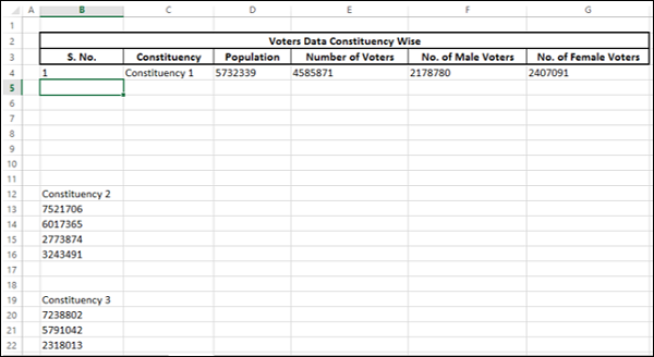
Предположим, вам необходимо проанализировать данные избирателей, собранных в 280 избирательных округах. Для каждого избирательного округа собраны следующие данные:
- Название избирательного округа.
- Общая численность населения в избирательном округе.
- Количество избирателей в избирательном округе.
- Количество избирателей мужского пола, и
- Количество женщин-избирателей.
Данные предоставляются вам на листе, как указано ниже.
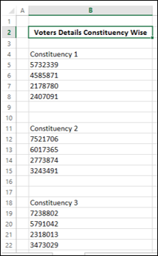
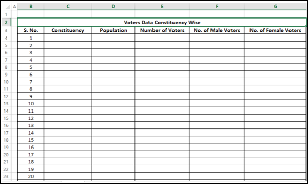
Невозможно проанализировать данные в вышеуказанном формате. Поэтому расположите данные в таблице, как показано ниже.
Если вы пытаетесь расположить данные в вышеуказанном формате –
Сбор данных из 280 избирательных округов занимает значительное время
Это может быть подвержено ошибкам
Это становится мирской задачей, не позволяющей вам сосредоточиться на технических вещах
Сбор данных из 280 избирательных округов занимает значительное время
Это может быть подвержено ошибкам
Это становится мирской задачей, не позволяющей вам сосредоточиться на технических вещах
Решение состоит в том, чтобы записать макрос, чтобы вы могли выполнить задачу не более, чем за несколько секунд. Макрос должен использовать относительные ссылки, так как вы будете перемещаться по строкам во время упорядочивания данных.
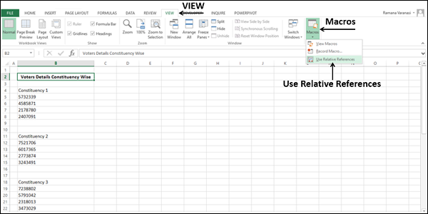
Использование относительных ссылок
Чтобы сообщить макрос-рекордеру, что он должен использовать относительные ссылки, сделайте следующее:
Нажмите вкладку VIEW на ленте.
Нажмите « Использовать относительные ссылки» .
Нажмите вкладку VIEW на ленте.
Нажмите « Использовать относительные ссылки» .
Подготовка формата данных
Первым шагом в организации приведенных выше данных является определение формата данных в таблице с заголовками.
Создайте строку заголовков, как показано ниже.
Запись макроса
Запишите макрос следующим образом –
Нажмите Запись макроса.
Дайте осмысленное имя, скажем, DataArrange макросу.
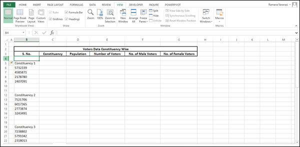
Тип = строка () – 3 в ячейке B4. Это потому, что номер S. является текущим номером строки – 3 строки над ним.
Разрежьте ячейки B5, B6, B7, B8 и B9 и вставьте их в ячейки C4-C8 соответственно.
Теперь нажмите на ячейку B5. Ваша таблица выглядит так, как показано ниже.
Нажмите Запись макроса.
Дайте осмысленное имя, скажем, DataArrange макросу.
Тип = строка () – 3 в ячейке B4. Это потому, что номер S. является текущим номером строки – 3 строки над ним.
Разрежьте ячейки B5, B6, B7, B8 и B9 и вставьте их в ячейки C4-C8 соответственно.
Теперь нажмите на ячейку B5. Ваша таблица выглядит так, как показано ниже.
Первый набор данных расположен в первой строке таблицы. Удалите строки B6 – B11 и щелкните в ячейке B5.
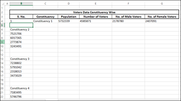
Вы можете видеть, что активная ячейка B5 и следующий набор данных будет размещен здесь.
Прекратите запись макроса. Ваш макрос для размещения данных готов.
Запуск макроса
Вам необходимо многократно запускать макрос, чтобы завершить размещение данных в таблице, как указано ниже.
Активная ячейка B5. Запустите макрос. Второй набор данных будет размещен во второй строке таблицы, а активной ячейкой будет B6.
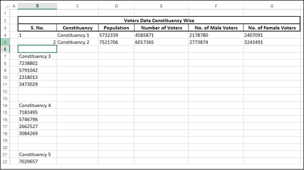
Запустите макрос снова. Третий набор данных будет размещен в третьей строке таблицы, и активной ячейкой станет B7.
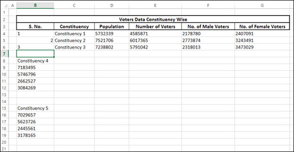
Каждый раз, когда вы запускаете макрос, активная ячейка продвигается к следующей строке, облегчая повторение записанных шагов в соответствующих позициях. Это возможно из-за относительных ссылок в макросе.
Запускайте макрос, пока все 280 наборов данных не будут объединены в 280 строк таблицы. Этот процесс занимает несколько секунд, и, поскольку шаги автоматизированы, все упражнение не содержит ошибок.
Источник
Использование макрорекордера. Абсолютные и относительные ссылки
1.2 Абсолютные и относительные ссылки
Запись абсолютных и относительных ссылок в формулах на рабочем листе
Например, если активна ячейка A4, то ссылку на ячейку D3 можно задать как D3 (стиль A1 ) или R[-1]C[3] (стиль R1C1 ).
При записи формулы в стиле A1 признаком абсолютной ссылки является знак доллара ($) перед адресом строки и/или столбца. В стиле R1C1 для задания абсолютной ссылки используются индексы ячейки. Например, на ячейку D3 указывает абсолютная ссылка $D$3 в стиле A1 и абсолютная ссылка R3C4 в стиле R1C1.
Запись абсолютных и относительных ссылок в процедурах VBA
В процедурах, создаваемых при помощи макрорекордера , абсолютные и относительные ссылки записываются в стиле R1C1.
По умолчанию после запуска макрорекодера кнопка отжата, что означает, что при записи процедур используются абсолютные ссылки.
Команда вычисления размера вклада в ячейке B13 с использованием абсолютных ссылок (набор адреса ячейки со знаками $ во время записи макроса ) будет выглядеть так:
Можно установить использование относительных ссылок при записи процедур Для этого после запуска макрорекордера нажмите кнопку Относительная ссылка на панели инструментов Остановить запись (см. рис. 1.2). Кнопка будет изображена на оранжевом фоне. Относительные ссылки будут использоваться до конца текущего сеанса работы в MS Excel или до повторного нажатия кнопки Относительная ссылка.
Другой способ задания относительных ссылок — использование свойства Offset объекта Range.
Источник
Как сделать относительную ссылку в excel для макроса?
По умолчанию, во время записи макроса, все действия по выбору ячеек и диапазонов записываются как абсолютные. Если Вы выбрали ячейку C5 и записали для нее какие-то манипуляции, то последующие воспроизведения макроса будут производить эти действия именно над этой ячейкой. Такое поведение не всегда может соответствовать имеющимся задачам.
Поэтому в приложение Excel предусмотрена специальная возможность записи макросов с относительными ссылками. Если перед запуском макрорекодера было включено данное свойство, то любые ссылки будут записываться как смещенные относительно той ячейки, которая была активна на может этого запуска. Если изначально была выделена ячейка A1, а затем выбрана ячейка C5, то в код макроса попадет такая запись:
Она указывает приложению на необходимость выделить ячейку, смещенную на 4 строки и 2 столбца от активной на данный момент ячейки. Это значит, если при последующем выполнении макроса предварительно выделить ячейку G10, то смещенной на 4 строки и 2 столбца окажется ячейка I14.
Для активации описанного параметра перейдите на вкладку «Вид», найдите область «Макросы» и в раскрывающемся меню кликните по пункту «Относительные ссылки».
Если материалы office-menu.ru Вам помогли, то поддержите, пожалуйста, проект, чтобы мы могли развивать его дальше.
У Вас недостаточно прав для комментирования.
Простую последовательность действий, которую нужно повторить несколько раз, можно записать в виде программного кода и сохранить как макрос. Если последовательность действий записана в макрос, то выполнять её можно снова и снова, просто запуская этот макрос. Это гораздо эффективнее, чем выполнять раз за разом одни и те же действия вручную.
Чтобы записать макрос, нужно включить режим записи. Это можно сделать на вкладке Вид (View) в разделе Макросы (Macros) или в меню Сервис (Tools), если у Вас Excel 2003. Ниже на картинках показано, как выглядят эти меню.
Далее откроется диалоговое окно Запись макроса (Record Macro), как показано на картинке ниже:

Здесь, по желанию, можно ввести имя и описание для макроса. Рекомендуется давать макросу такое имя, чтобы, вернувшись к нему спустя некоторое время, можно было без труда понять, для чего этот макрос нужен. Так или иначе, если не ввести для макроса имя, то Excel автоматически назовёт его Макрос1, Макрос2 и так далее.
Здесь же можно назначить сочетание клавиш для запуска записанного макроса. Запускать макрос таким способом будет значительно проще. Однако будьте осторожны! Если случайно назначить для макроса одно из предустановленных клавиатурных сочетаний Excel (например, Ctrl+C), то в дальнейшем макрос может быть запущен случайно.
Когда макросу дано подходящее имя и (при желании) задано сочетание клавиш, нажмите ОК, чтобы запустить запись макроса. С этого момента каждое действие (ввод данных, выделение ячеек, изменение формата ячеек, пролистывание листа и так далее) будет записано в макрос и сохранено в виде кода VBA.
При включении режима записи макроса в строке состояния (внизу слева) появляется кнопка Стоп. В Excel 2003 эта кнопка находится на плавающей панели инструментов.
Нажмите Стоп, когда выполните все действия, которые должны быть записаны в макрос. Теперь код записанного макроса сохранён в модуле редактора Visual Basic.
Параметр «Относительные ссылки»
Если перед началом записи макроса включить параметр Относительные ссылки (Use Relative References), то все ссылки в записываемом макросе будут создаваться как относительные. Если же параметр выключен, то при записи макроса будут создаваться абсолютные ссылки (подробнее об этих двух типах ссылок можно узнать в статьях, посвящённых теме ссылок на ячейки в Excel).
Параметр Относительные ссылки (Use Relative References) находится в разделе Макросы (Macros) на вкладке Вид (View). В Excel 2003 этот параметр расположен на плавающей панели инструментов.
Просмотр кода VBA
Код VBA, записанный в макрос, размещается в модуле, который можно просмотреть в редакторе Visual Basic. Редактор можно запустить нажатием Alt+F11 (одновременное нажатие клавиш Alt и F11).
Код находится в одном из модулей, которые расположены в окне Project слева от области редактирования. Если дважды кликнуть по Module1 в окне Project, то справа появится код записанного макроса.
Запуск записанного макроса в Excel
Записывая макрос, Excel всегда создаёт процедуру Sub (не Function). Если при создании макроса к нему было прикреплено сочетание клавиш, то именно с его помощью запустить макрос будет проще всего. Существует и другой способ запустить макрос:
- Нажмите Alt+F8 (одновременно нажмите клавиши Alt и F8);
- В появившемся списке макросов выберите тот, который нужно запустить;
- Нажмите кнопку Выполнить (Run).
Ограничения
Инструмент Excel для записи макросов – это очень простой способ создавать код VBA, но подходит он только для создания самых простых макросов. Дело в том, что этот инструмент не умеет использовать многие возможности VBA, такие как:
- Константы, переменные и массивы;
- Выражения IF;
- Циклы;
- Обращения к встроенным функциям или внешним процедурам.
Как уже было сказано, инструмент записи макросов может создавать только процедуры Sub, так как не может возвращать значение. Процедурам Sub нельзя передавать какие-либо аргументы, хотя они могут распознавать текущие активные ячейки, диапазоны или листы, а также значения, хранящиеся в ячейках книги. Кроме того, нужно сказать, что сгенерированный код не всегда является оптимальным для рассматриваемой последовательности действий.
Автоматическое создание кода VBA в Excel отлично работает для простых макросов, но если нужно построить более сложный макрос, то придётся научиться писать код VBA самостоятельно. Тем не менее, запись макроса в Excel – это отличны инструмент, при помощи которого можно создавать первоначальный код, а в дальнейшем исправлять или вставлять его в более сложные макросы.
Урок подготовлен для Вас командой сайта office-guru.ru
Источник:/> Перевел: Антон Андронов
Правила перепечаткиЕще больше уроков по Microsoft Excel
Оцените качество статьи. Нам важно ваше мнение:
Разберемся как сделать все ссылки абсолютными, относительными или смешанными в диапазоне ячеек в Excel, а не только для одной конкретной ссылки в формуле.
Приветствую всех, дорогие читатели блога TutorExcel.Ru.
Как мы уже хорошо знаем всего в Excel выделяют 3 типа ссылок: относительные (А1), абсолютные ($А$1) и смешанные ($А1 и А$1).
Применение каждого из типов имеет свой смысл и определенные преимущества, поэтому зачастую бывает полезно в формулах заменить все относительные ссылки на абсолютные (или наоборот), к примеру, часто может пригодиться при копировании диапазона ячеек.
Поменять тип для конкретной ссылки в ячейке можно с помощью клавиши F4.
Для этого выделяем ссылку в формуле (либо на ячейку, либо на диапазон ячеек) и поочередно нажимаем F4, в результате ссылки будут меняться в порядке A1 -> $A$1 -> $A1 -> A$1. Затем останавливаемся на нужном шаге и задача смены типа решена.
Однако как это нередко случается в Excel, что удобно сделать 1 раз, не совсем удобно делать десятки, а то и сотни раз.
Так с помощью клавиши F4 мы сможем быстро изменить тип для одной ссылки, но никак не для большого диапазона ячеек с данными.
Поэтому чтобы проделать эту операцию вручную для множества ссылок потребуется другой способ (представьте сколько у вас займет времени поменять ссылки в 100 ячейках), в связи с чем обратимся к помощи макроса, который автоматизирует процесс и существенно ускорит время выполнения работы.
Как поменять ссылки в формулах на абсолютные?
Алгоритм действия макроса построим по следующему принципу: мы заходим в каждую ячейку диапазона, где содержится формула, а далее преобразовываем ссылку в нужный нам вид.
На словах все выглядит просто, давайте перейдем к реализации алгоритма.
Переходим в редактор VBA (для быстрого перехода нажимаем Alt + F11), создаем новый модуль (щелкаем правой кнопкой мыши в панели проектов и выбираем Insert -> Module) и добавляем туда код макроса:
Dim MyCell As Range
On Error Resume Next ‘Обработка ошибки, если рассматриваемый диапазон ячеек не содержит формул
For Each MyCell In Selection.SpecialCells(xlCellTypeFormulas) ‘Цикл для каждой ячейки диапазона содержащая формулу
MyCell.Formula = Application.ConvertFormula(MyCell.Formula, xlA1, xlA1, xlAbsolute) ‘Меняем тип ссылки
Попробуем проверить работу макроса на простой таблице с формулами:


Выделяем диапазон ячеек с таблицей (в нашем случае это диапазон F6:J10) и запускаем макрос ChangeCellStyleInFormulas (в панели вкладок выбираем Разработчик -> Макросы (или нажимаем Alt + F8), далее находим нужный макрос и жмем Выполнить):

Все получилось, ссылки в таблице из относительных преобразовались в абсолютные.
Теперь рассмотрим другие случаи, когда в конечном результате нужны уже не абсолютные, а относительные или смешанные ссылки.
Как поменять ссылки в формулах на относительные?
За преобразование формулы в макросе отвечает функция ConvertFormula, в которой один из параметров задает тип ссылки:
- xlAbsolute. Абсолютная ($А$1);
- xlRelative. Относительная (А1);
- xlAbsRowRelColumn. Смешанная. Абсолютная строка и относительный столбец (А$1);
- xlRelRowAbsColumn. Смешанная. Относительная строка и абсолютный столбец ($А1).
Поэтому вместо xlAbsolute в коде макроса можно поставить любой из выше перечисленных параметров, в зависимости от того, что конкретно вам нужно.
Например, для той же таблицы применим макрос с параметром xlAbsRowRelColumn (абсолютная строка и относительный столбец, вид A$1):

И для параметра xlRelRowAbsColumn (относительная строка и абсолютный столбец, вид $A1):

Таким образом, меняя значения параметра в макросе можно получить абсолютно любой тип ссылки.
Способ преобразования без использования макросов
Если не хочется возиться с макросами, то преобразовать все ссылки в формулах в относительные также можно и без их применения.
Действительно, так как признаком абсолютной или смешанной ссылки является наличие в формуле знака $ (который используется для закрепления строки или столбца), то с помощью инструмента Найти и заменить можно избавиться от всех знаков $ в формулах.
Выделяем диапазон с данными, нажимаем Ctrl + H, в поле Найти указываем знак доллара, а поле Заменить на оставляем пустым, нажимаем Заменить все и получаем нужный результат:

Замечания
Будьте внимательны при работе с формулами массива, после работы макроса они превращаются в обычные и могут вернуть значение ошибки. Также из-за особенностей VBA макрос может некорректно обрабатывать большие по объему формулы.
Спасибо за внимание!
Если у вас есть мысли или вопросы по теме статьи — пишите в комментариях.
Источник
Хитрости »
19 Февраль 2021 6745 просмотров
Использование относительных ссылок в макросах
Если Вы уже записывали макросы обработки таблиц, то наверняка сталкивались с ситуацией, когда макросом в таблицу добавляется столбец с формулами, которые потом необходимо распространить на все строки. Но если количество строк в таблице изменяется, то макрос работает некорректно: если строк стало больше, то формулы проставляются не на все строки, а если строк стало меньше – то появляются строки с лишними формулами.
Если Вы еще не знаете что такое макрос и как его записывать и воспроизводить, то рекомендуется сначала ознакомиться со статьей: Что такое макрос и где его искать?
К примеру, возьмем таблицу такого вида:

В конце таблицы нам необходимо добавить столбец «Стоимость», прописав в нем нехитрую формулу перемножения количества на цену:
=F2*G2
Перед записью макроса выделяем ячейку H1. При обычной записи макроса наши шаги такие:
1. Выделили I1
2. Записали в неё заголовок «Стоимость»
3. Перешли в I2
4. Записали формулу: =F2*G2
5. Распространили формулу до конца таблицы (через автозаполнение или путем копирования ячейки с формулой и вставки в остальные ячейки)
Макрос работает отлично. Пока количество строк не изменится. Если при записи макроса в таблице было 319 строк, а потом добавилось еще 20, то записанный макрос создаст формулу только в первых 319 строках. Все дело в том, что при обычной записи макрос использует абсолютную адресацию ячеек. Т.е. в нем каждый наш шаг обозначает выделение ячеек с конкретно указанным адресом (I1, I2, I319 и т.д.):

Как выйти из такой ситуации? Все не слишком сложно. В группе кнопок код на вкладке Разработчик есть кнопка «Относительные ссылки». Если нажать её до записи макроса(или во время), то ссылки на ячейки будут уже запоминаться не как конкретный адрес, а как смещение относительно последней выделенной ячейки.
Например, запишем два простых макроса, которые будут делать одно и то же действие – перемещение вниз таблицы и выделение ячеек от нижней до верхней. Только первый макрос будет записан обычным способом, а перед записью второго мы нажмем кнопку «Относительные ссылки». Наши действия будут следующими (одинаковыми для обоих макросов):
1. До записи макроса выделяем ячейку I2
2. Начинаем запись макроса
3. Выделяем ячейку H2
4. Комбинацией клавиш Ctrl+↓(стрелка вниз) перемещаемся вниз таблицы
5. Стрелка вправо (т.е. выделяем последнюю ячейку в столбце I)
6. Комбинацией клавиш Ctrl+Shift+↑(стрелка вверх) выделяем столбец I от последней ячейки до первой
7. Завершаем запись макроса
Теперь можно посмотреть на код обоих макросов:

Отличия очевидны: в первом используется обращение к ячейкам по их конкретным адресам. Во втором же все действия происходят относительно последней выделенной ячейки(на Range(«A1») не обращаем внимания – это из другой оперы и если их удалить ничего не изменится). Из этого можно сделать вывод, что для создания гибких универсальных макросов с использованием относительных ссылок необходимо как можно меньше использовать мышку и максимально стараться применять горячие клавиши. Попробую пояснить почему: когда мы применяем то же автозаполнение (наведение курсора мыши на нижний правый угол ячейки и протягивание вниз или двойной щелчок левой кнопкой мыши) – оно применяется к конкретно определенному количеству ячеек. Т.е. даже относительные ссылки не помогут заполнить его формулами, как того требует наша изначальная задача. Но если использовать горячие клавиши перемещения и выделения (Ctrl+стрелка и Ctrl+Shift+стрелка), то мы можем создать макрос, которому уже будет не важно сколько строк в нашей таблице. Чтобы в этом убедиться, запишем макрос из начала статьи, но уже с использованием относительных ссылок и исключительно клавиш для перемещения. Наши действия:
1. Перед записью макроса выделяем ячейку H1
2. Начали запись макроса
3. Нажимаем кнопку Относительные ссылки(если она еще не нажата)
4. Выделяем I1
5. Записываем в неё заголовок «Стоимость»
6. Переходим в I2
7. Записываем в I2 формулу: =F2*G2
8. Комбинацией клавиш Ctrl+C(или при помощи контекстного меню мыши) копируем ячейку с формулой
9. Стрелкой вправо перемещаемся в ячейку H2
10. Комбинацией клавиш Ctrl+↓(стрелка вниз) перемещаемся вниз таблицы
11. Стрелка вправо (т.е. выделяем последнюю ячейку в столбце I)
12. Комбинацией клавиш Ctrl+Shift+↑(стрелка вверх) выделяем столбец I от последней ячейки до первой
13. Комбинацией клавиш Ctrl+V вставляем скопированную формулу
14. Нажимаем Esc для сброса буфера обмена
15. Запись макроса можно завершить
Если теперь попробовать применить такой макрос к таблице, у которой строк больше или меньше, чем было при записи макроса – все пройдет идеально. Макрос создаст столбец и запишет в нем формулу только на нужное количество строк.
Более того. Если наша таблица находится уже в другом листе и даже начинается не с первой ячейки, а где-то в середине:

Нам достаточно будет выделить ячейку заголовка последнего столбца(K5) и запустить наш макрос. Он без проблем добавит столбец с формулой в нужном месте и на все строки. Макрос же без использования относительных ссылок в такой ситуации спасует по полной: он создаст формулы начиная с ячейки I2 и до заголовка, только испортив таблицу и не сделав ничего полезного.
Так же хочу дополнить, что Относительные ссылки играют роль исключительно во время записи макроса. Во время воспроизведения совершенно не важно включены они или нет. Плюс можно(а иногда и нужно) комбинировать во время записи макросов режим относительных ссылок с обычным режимом. Например, когда столбцов в таблице у нас всегда одинаковое количество и таблица всегда в одном месте, и столбец мы добавляем всегда в столбец I. Но формулы при этом надо протягивать на разное количество строк. Тогда можно начать запись макроса обычным режимом, а после того, как записали название столбца — включить режим относительных ссылок, чтобы определение последней ячейки таблицы не зависело от количества строк в этой таблице.
Статья помогла? Поделись ссылкой с друзьями!
![]() Видеоуроки
Видеоуроки
Поиск по меткам
Access
apple watch
Multex
Power Query и Power BI
VBA управление кодами
Бесплатные надстройки
Дата и время
Записки
ИП
Надстройки
Печать
Политика Конфиденциальности
Почта
Программы
Работа с приложениями
Разработка приложений
Росстат
Тренинги и вебинары
Финансовые
Форматирование
Функции Excel
акции MulTEx
ссылки
статистика
In this Article
- Ranges and Cells in VBA
- Cell Address
- Range of Cells
- Writing to Cells
- Reading from Cells
- Non Contiguous Cells
- Intersection of Cells
- Offset from a Cell or Range
- Setting Reference to a Range
- Resize a Range
- OFFSET vs Resize
- All Cells in Sheet
- UsedRange
- CurrentRegion
- Range Properties
- Last Cell in Sheet
- Last Used Row Number in a Column
- Last Used Column Number in a Row
- Cell Properties
- Copy and Paste
- AutoFit Contents
- More Range Examples
- For Each
- Sort
- Find
- Range Address
- Range to Array
- Array to Range
- Sum Range
- Count Range
Ranges and Cells in VBA
Excel spreadsheets store data in Cells. Cells are arranged into Rows and Columns. Each cell can be identified by the intersection point of it’s row and column (Exs. B3 or R3C2).
An Excel Range refers to one or more cells (ex. A3:B4)
Cell Address
A1 Notation
In A1 notation, a cell is referred to by it’s column letter (from A to XFD) followed by it’s row number(from 1 to 1,048,576). This is called a cell address.
In VBA you can refer to any cell using the Range Object.
' Refer to cell B4 on the currently active sheet
MsgBox Range("B4")

' Refer to cell B4 on the sheet named 'Data'
MsgBox Worksheets("Data").Range("B4")

' Refer to cell B4 on the sheet named 'Data' in another OPEN workbook
' named 'My Data'
MsgBox Workbooks("My Data").Worksheets("Data").Range("B4")
R1C1 Notation
In R1C1 Notation a cell is referred by R followed by Row Number then letter ‘C’ followed by the Column Number. eg B4 in R1C1 notation will be referred by R4C2. In VBA you use the Cells Object to use R1C1 notation:
' Refer to cell R[6]C[4] i.e D6
Cells(6, 4) = "D6"
Range of Cells
A1 Notation
To refer to a more than one cell use a “:” between the starting cell address and last cell address. The following will refer to all the cells from A1 to D10:
Range("A1:D10")
R1C1 Notation
To refer to a more than one cell use a “,” between the starting cell address and last cell address. The following will refer to all the cells from A1 to D10:
Range(Cells(1, 1), Cells(10, 4))Writing to Cells
To write values to a cell or contiguous group of cells, simple refer to the range, put an = sign and then write the value to be stored:
' Store F5 in cell with Address F6
Range("F6") = "F6"

' Store E6 in cell with Address R[6]C[5] i.e E6
Cells(6, 5) = "E6"

' Store A1:D10 in the range A1:D10
Range("A1:D10") = "A1:D10"
' or
Range(Cells(1, 1), Cells(10, 4)) = "A1:D10"
Reading from Cells
To read values from cells, simple refer to the variable to store the values, put an = sign and then refer to the range to be read:
Dim val1
Dim val2

' Read from cell F6
val1 = Range("F6")

' Read from cell E6
val2 = Cells(6, 5)

MsgBox val1
Msgbox val2
Note: To store values from a range of cells, you need to use an Array instead of a simple variable.
Non Contiguous Cells
To refer to non contiguous cells use a comma between the cell addresses:
' Store 10 in cells A1, A3, and A5
Range("A1,A3,A5") = 10


' Store 10 in cells A1:A3 and D1:D3)
Range("A1:A3, D1:D3") = 10
VBA Coding Made Easy
Stop searching for VBA code online. Learn more about AutoMacro — A VBA Code Builder that allows beginners to code procedures from scratch with minimal coding knowledge and with many time-saving features for all users!

Learn More
Intersection of Cells
To refer to non contiguous cells use a space between the cell addresses:
' Store 'Col D' in D1:D10
' which is Common between A1:D10 and D1:F10
Range("A1:D10 D1:G10") = "Col D"
Offset from a Cell or Range
Using the Offset function, you can move the reference from a given Range (cell or group of cells) by the specified number_of_rows, and number_of_columns.
Offset Syntax
Range.Offset(number_of_rows, number_of_columns)
Offset from a cell
' OFFSET from a cell A1
' Refer to cell itself
' Move 0 rows and 0 columns
Range("A1").Offset(0, 0) = "A1"

' Move 1 rows and 0 columns
Range("A1").Offset(1, 0) = "A2"

' Move 0 rows and 1 columns
Range("A1").Offset(0, 1) = "B1"

' Move 1 rows and 1 columns
Range("A1").Offset(1, 1) = "B2"

' Move 10 rows and 5 columns
Range("A1").Offset(10, 5) = "F11"
Offset from a Range
' Move Reference to Range A1:D4 by 4 rows and 4 columns
' New Reference is E5:H8
Range("A1:D4").Offset(4,4) = "E5:H8"
Setting Reference to a Range
To assign a range to a range variable: declare a variable of type Range then use the Set command to set it to a range. Please note that you must use the SET command as RANGE is an object:
' Declare a Range variable
Dim myRange as Range

' Set the variable to the range A1:D4
Set myRange = Range("A1:D4")

' Prints $A$1:$D$4
MsgBox myRange.Address
VBA Programming | Code Generator does work for you!
Resize a Range
Resize method of Range object changes the dimension of the reference range:
Dim myRange As Range

' Range to Resize
Set myRange = Range("A1:F4")

' Prints $A$1:$E$10
Debug.Print myRange.Resize(10, 5).Address
Top-left cell of the Resized range is same as the top-left cell of the original range
Resize Syntax
Range.Resize(number_of_rows, number_of_columns)
OFFSET vs Resize
Offset does not change the dimensions of the range but moves it by the specified number of rows and columns. Resize does not change the position of the original range but changes the dimensions to the specified number of rows and columns.
All Cells in Sheet
The Cells object refers to all the cells in the sheet (1048576 rows and 16384 columns).
' Clear All Cells in Worksheets
Cells.Clear
UsedRange
UsedRange property gives you the rectangular range from the top-left cell used cell to the right-bottom used cell of the active sheet.
Dim ws As Worksheet
Set ws = ActiveSheet

' $B$2:$L$14 if L2 is the first cell with any value
' and L14 is the last cell with any value on the
' active sheet
Debug.Print ws.UsedRange.Address
CurrentRegion
CurrentRegion property gives you the contiguous rectangular range from the top-left cell to the right-bottom used cell containing the referenced cell/range.
Dim myRange As Range

Set myRange = Range("D4:F6")

' Prints $B$2:$L$14
' If there is a filled path from D4:F16 to B2 AND L14
Debug.Print myRange.CurrentRegion.Address

' You can refer to a single starting cell also

Set myRange = Range("D4") ' Prints $B$2:$L$14
AutoMacro | Ultimate VBA Add-in | Click for Free Trial!
Range Properties
You can get Address, row/column number of a cell, and number of rows/columns in a range as given below:
Dim myRange As Range

Set myRange = Range("A1:F10")

' Prints $A$1:$F$10
Debug.Print myRange.Address

Set myRange = Range("F10")

' Prints 10 for Row 10
Debug.Print myRange.Row

' Prints 6 for Column F
Debug.Print myRange.Column

Set myRange = Range("E1:F5")
' Prints 5 for number of Rows in range
Debug.Print myRange.Rows.Count

' Prints 2 for number of Columns in range
Debug.Print myRange.Columns.Count
Last Cell in Sheet
You can use Rows.Count and Columns.Count properties with Cells object to get the last cell on the sheet:
' Print the last row number
' Prints 1048576
Debug.Print "Rows in the sheet: " & Rows.Count

' Print the last column number
' Prints 16384
Debug.Print "Columns in the sheet: " & Columns.Count

' Print the address of the last cell
' Prints $XFD$1048576
Debug.Print "Address of Last Cell in the sheet: " & Cells(Rows.Count, Columns.Count)
Last Used Row Number in a Column
END property takes you the last cell in the range, and End(xlUp) takes you up to the first used cell from that cell.
Dim lastRow As Long

lastRow = Cells(Rows.Count, "A").End(xlUp).Row
Last Used Column Number in a Row
Dim lastCol As Long

lastCol = Cells(1, Columns.Count).End(xlToLeft).Column
END property takes you the last cell in the range, and End(xlToLeft) takes you left to the first used cell from that cell.
You can also use xlDown and xlToRight properties to navigate to the first bottom or right used cells of the current cell.
AutoMacro | Ultimate VBA Add-in | Click for Free Trial!
Cell Properties
Common Properties
Here is code to display commonly used Cell Properties
Dim cell As Range
Set cell = Range("A1")

cell.Activate
Debug.Print cell.Address
' Print $A$1

Debug.Print cell.Value
' Prints 456
' Address

Debug.Print cell.Formula
' Prints =SUM(C2:C3)

' Comment
Debug.Print cell.Comment.Text

' Style
Debug.Print cell.Style

' Cell Format
Debug.Print cell.DisplayFormat.NumberFormat
Cell Font
Cell.Font object contains properties of the Cell Font:
Dim cell As Range

Set cell = Range("A1")

' Regular, Italic, Bold, and Bold Italic
cell.Font.FontStyle = "Bold Italic"
' Same as
cell.Font.Bold = True
cell.Font.Italic = True

' Set font to Courier
cell.Font.FontStyle = "Courier"

' Set Font Color
cell.Font.Color = vbBlue
' or
cell.Font.Color = RGB(255, 0, 0)

' Set Font Size
cell.Font.Size = 20
Copy and Paste
Paste All
Ranges/Cells can be copied and pasted from one location to another. The following code copies all the properties of source range to destination range (equivalent to CTRL-C and CTRL-V)
'Simple Copy
Range("A1:D20").Copy
Worksheets("Sheet2").Range("B10").Paste

'or
' Copy from Current Sheet to sheet named 'Sheet2'
Range("A1:D20").Copy destination:=Worksheets("Sheet2").Range("B10")
Paste Special
Selected properties of the source range can be copied to the destination by using PASTESPECIAL option:
' Paste the range as Values only
Range("A1:D20").Copy
Worksheets("Sheet2").Range("B10").PasteSpecial Paste:=xlPasteValues
Here are the possible options for the Paste option:
' Paste Special Types
xlPasteAll
xlPasteAllExceptBorders
xlPasteAllMergingConditionalFormats
xlPasteAllUsingSourceTheme
xlPasteColumnWidths
xlPasteComments
xlPasteFormats
xlPasteFormulas
xlPasteFormulasAndNumberFormats
xlPasteValidation
xlPasteValues
xlPasteValuesAndNumberFormats
AutoFit Contents
Size of rows and columns can be changed to fit the contents using AutoFit:
' Change size of rows 1 to 5 to fit contents
Rows("1:5").AutoFit

' Change size of Columns A to B to fit contents
Columns("A:B").AutoFit
More Range Examples
It is recommended that you use Macro Recorder while performing the required action through the GUI. It will help you understand the various options available and how to use them.
AutoMacro | Ultimate VBA Add-in | Click for Free Trial!
For Each
It is easy to loop through a range using For Each construct as show below:
For Each cell In Range("A1:B100")
    ' Do something with the cell
Next cell
At each iteration of the loop one cell in the range is assigned to the variable cell and statements in the For loop are executed for that cell. Loop exits when all the cells are processed.
Sort
Sort is a method of Range object. You can sort a range by specifying options for sorting to Range.Sort. The code below will sort the columns A:C based on key in cell C2. Sort Order can be xlAscending or xlDescending. Header:= xlYes should be used if first row is the header row.
   Columns("A:C").Sort key1:=Range("C2"), _
      order1:=xlAscending, Header:=xlYes
Find
Find is also a method of Range Object. It find the first cell having content matching the search criteria and returns the cell as a Range object. It return Nothing if there is no match.
Use FindNext method (or FindPrevious) to find next(previous) occurrence.
Following code will change the font to “Arial Black” for all cells in the range which start with “John”:
For Each c In Range("A1:A100")
    If c Like "John*" Then
        c.Font.Name = "Arial Black"
    End If
Next c
Following code will replace all occurrences of “To Test” to “Passed” in the range specified:
With Range("a1:a500")
    Set c = .Find("To Test", LookIn:=xlValues)
    If Not c Is Nothing Then
        firstaddress = c.Address
        Do
            c.Value = "Passed"
            Set c = .FindNext(c)
        Loop While Not c Is Nothing And c.Address <> firstaddress
    End If
End With
It is important to note that you must specify a range to use FindNext. Also you must provide a stopping condition otherwise the loop will execute forever. Normally address of the first cell which is found is stored in a variable and loop is stopped when you reach that cell again. You must also check for the case when nothing is found to stop the loop.
Range Address
Use Range.Address to get the address in A1 Style
MsgBox Range("A1:D10").Address
' or
Debug.Print Range("A1:D10").Address
Use xlReferenceStyle (default is xlA1) to get addres in R1C1 style
MsgBox Range("A1:D10").Address(ReferenceStyle:=xlR1C1)
' or
Debug.Print Range("A1:D10").Address(ReferenceStyle:=xlR1C1)
This is useful when you deal with ranges stored in variables and want to process for certain addresses only.
AutoMacro | Ultimate VBA Add-in | Click for Free Trial!
Range to Array
It is faster and easier to transfer a range to an array and then process the values. You should declare the array as Variant to avoid calculating the size required to populate the range in the array. Array’s dimensions are set to match number of values in the range.
Dim DirArray As Variant
' Store the values in the range to the Array

DirArray = Range("a1:a5").Value

' Loop to process the values
For Each c In DirArray
    Debug.Print c
Next
Array to Range
After processing you can write the Array back to a Range. To write the Array in the example above to a Range you must specify a Range whose size matches the number of elements in the Array.
Use the code below to write the Array to the range D1:D5:
Range("D1:D5").Value = DirArray

Range("D1:H1").Value = Application.Transpose(DirArray)
Please note that you must Transpose the Array if you write it to a row.
Sum Range
SumOfRange = Application.WorksheetFunction.Sum(Range("A1:A10"))
Debug.Print SumOfRange
You can use many functions available in Excel in your VBA code by specifying Application.WorkSheetFunction. before the Function Name as in the example above.
Count Range
' Count Number of Cells with Numbers in the Range
CountOfCells = Application.WorksheetFunction.Count(Range("A1:A10"))
Debug.Print CountOfCells

' Count Number of Non Blank Cells in the Range
CountOfNonBlankCells = Application.WorksheetFunction.CountA(Range("A1:A10"))
Debug.Print CountOfNonBlankCells
Written by: Vinamra Chandra
“It is a capital mistake to theorize before one has data”- Sir Arthur Conan Doyle
This post covers everything you need to know about using Cells and Ranges in VBA. You can read it from start to finish as it is laid out in a logical order. If you prefer you can use the table of contents below to go to a section of your choice.
Topics covered include Offset property, reading values between cells, reading values to arrays and formatting cells.
A Quick Guide to Ranges and Cells
| Function | Takes | Returns | Example | Gives |
|---|---|---|---|---|
|
Range |
cell address | multiple cells | .Range(«A1:A4») | $A$1:$A$4 |
| Cells | row, column | one cell | .Cells(1,5) | $E$1 |
| Offset | row, column | multiple cells | Range(«A1:A2») .Offset(1,2) |
$C$2:$C$3 |
| Rows | row(s) | one or more rows | .Rows(4) .Rows(«2:4») |
$4:$4 $2:$4 |
| Columns | column(s) | one or more columns | .Columns(4) .Columns(«B:D») |
$D:$D $B:$D |
Download the Code
The Webinar
If you are a member of the VBA Vault, then click on the image below to access the webinar and the associated source code.
(Note: Website members have access to the full webinar archive.)

Introduction
This is the third post dealing with the three main elements of VBA. These three elements are the Workbooks, Worksheets and Ranges/Cells. Cells are by far the most important part of Excel. Almost everything you do in Excel starts and ends with Cells.
Generally speaking, you do three main things with Cells
- Read from a cell.
- Write to a cell.
- Change the format of a cell.
Excel has a number of methods for accessing cells such as Range, Cells and Offset.These can cause confusion as they do similar things and can lead to confusion
In this post I will tackle each one, explain why you need it and when you should use it.
Let’s start with the simplest method of accessing cells – using the Range property of the worksheet.
Important Notes
I have recently updated this article so that is uses Value2.
You may be wondering what is the difference between Value, Value2 and the default:
' Value2
Range("A1").Value2 = 56

' Value
Range("A1").Value = 56

' Default uses value
Range("A1") = 56
Using Value may truncate number if the cell is formatted as currency. If you don’t use any property then the default is Value.
It is better to use Value2 as it will always return the actual cell value(see this article from Charle Williams.)
The Range Property
The worksheet has a Range property which you can use to access cells in VBA. The Range property takes the same argument that most Excel Worksheet functions take e.g. “A1”, “A3:C6” etc.
The following example shows you how to place a value in a cell using the Range property.
' https://excelmacromastery.com/
Public Sub WriteToCell()

    ' Write number to cell A1 in sheet1 of this workbook
    ThisWorkbook.Worksheets("Sheet1").Range("A1").Value2 = 67

    ' Write text to cell A2 in sheet1 of this workbook
    ThisWorkbook.Worksheets("Sheet1").Range("A2").Value2 = "John Smith"

    ' Write date to cell A3 in sheet1 of this workbook
    ThisWorkbook.Worksheets("Sheet1").Range("A3").Value2 = #11/21/2017#

End Sub
As you can see Range is a member of the worksheet which in turn is a member of the Workbook. This follows the same hierarchy as in Excel so should be easy to understand. To do something with Range you must first specify the workbook and worksheet it belongs to.
For the rest of this post I will use the code name to reference the worksheet.

The following code shows the above example using the code name of the worksheet i.e. Sheet1 instead of ThisWorkbook.Worksheets(“Sheet1”).
' https://excelmacromastery.com/
Public Sub UsingCodeName()

    ' Write number to cell A1 in sheet1 of this workbook
    Sheet1.Range("A1").Value2 = 67

    ' Write text to cell A2 in sheet1 of this workbook
    Sheet1.Range("A2").Value2 = "John Smith"

    ' Write date to cell A3 in sheet1 of this workbook
    Sheet1.Range("A3").Value2 = #11/21/2017#

End Sub
You can also write to multiple cells using the Range property
' https://excelmacromastery.com/
Public Sub WriteToMulti()

    ' Write number to a range of cells
    Sheet1.Range("A1:A10").Value2 = 67

    ' Write text to multiple ranges of cells
    Sheet1.Range("B2:B5,B7:B9").Value2 = "John Smith"

End Sub
You can download working examples of all the code from this post from the top of this article.
The Cells Property of the Worksheet
The worksheet object has another property called Cells which is very similar to range. There are two differences
- Cells returns a range of one cell only.
- Cells takes row and column as arguments.
The example below shows you how to write values to cells using both the Range and Cells property
' https://excelmacromastery.com/
Public Sub UsingCells()

    ' Write to A1
    Sheet1.Range("A1").Value2 = 10
    Sheet1.Cells(1, 1).Value2  = 10

    ' Write to A10
    Sheet1.Range("A10").Value2 = 10
    Sheet1.Cells(10, 1).Value2  = 10

    ' Write to E1
    Sheet1.Range("E1").Value2 = 10
    Sheet1.Cells(1, 5).Value2  = 10

End Sub
You may be wondering when you should use Cells and when you should use Range. Using Range is useful for accessing the same cells each time the Macro runs.
For example, if you were using a Macro to calculate a total and write it to cell A10 every time then Range would be suitable for this task.
Using the Cells property is useful if you are accessing a cell based on a number that may vary. It is easier to explain this with an example.
In the following code, we ask the user to specify the column number. Using Cells gives us the flexibility to use a variable number for the column.
' https://excelmacromastery.com/
Public Sub WriteToColumn()

    Dim UserCol As Integer

    ' Get the column number from the user
    UserCol = Application.InputBox(" Please enter the column...", Type:=1)

    ' Write text to user selected column
    Sheet1.Cells(1, UserCol).Value2 = "John Smith"

End Sub
In the above example, we are using a number for the column rather than a letter.
To use Range here would require us to convert these values to the letter/number cell reference e.g. “C1”. Using the Cells property allows us to provide a row and a column number to access a cell.
Sometimes you may want to return more than one cell using row and column numbers. The next section shows you how to do this.
Using Cells and Range together
As you have seen you can only access one cell using the Cells property. If you want to return a range of cells then you can use Cells with Ranges as follows
' https://excelmacromastery.com/
Public Sub UsingCellsWithRange()

    With Sheet1
        ' Write 5 to Range A1:A10 using Cells property
        .Range(.Cells(1, 1), .Cells(10, 1)).Value2 = 5

        ' Format Range B1:Z1 to be bold
        .Range(.Cells(1, 2), .Cells(1, 26)).Font.Bold = True

    End With

End Sub
As you can see, you provide the start and end cell of the Range. Sometimes it can be tricky to see which range you are dealing with when the value are all numbers. Range has a property called Address which displays the letter/ number cell reference of any range. This can come in very handy when you are debugging or writing code for the first time.
In the following example we print out the address of the ranges we are using:
' https://excelmacromastery.com/
Public Sub ShowRangeAddress()

    ' Note: Using underscore allows you to split up lines of code
    With Sheet1

        ' Write 5 to Range A1:A10 using Cells property
        .Range(.Cells(1, 1), .Cells(10, 1)).Value2 = 5
        Debug.Print "First address is : " _
            + .Range(.Cells(1, 1), .Cells(10, 1)).Address

        ' Format Range B1:Z1 to be bold
        .Range(.Cells(1, 2), .Cells(1, 26)).Font.Bold = True
        Debug.Print "Second address is : " _
            + .Range(.Cells(1, 2), .Cells(1, 26)).Address

    End With

End Sub
In the example I used Debug.Print to print to the Immediate Window. To view this window select View->Immediate Window(or Ctrl G)


You can download all the code for this post from the top of this article.
The Offset Property of Range
Range has a property called Offset. The term Offset refers to a count from the original position. It is used a lot in certain areas of programming. With the Offset property you can get a Range of cells the same size and a certain distance from the current range. The reason this is useful is that sometimes you may want to select a Range based on a certain condition. For example in the screenshot below there is a column for each day of the week. Given the day number(i.e. Monday=1, Tuesday=2 etc.) we need to write the value to the correct column.

We will first attempt to do this without using Offset.
' https://excelmacromastery.com/
' This sub tests with different values
Public Sub TestSelect()

    ' Monday
    SetValueSelect 1, 111.21
    ' Wednesday
    SetValueSelect 3, 456.99
    ' Friday
    SetValueSelect 5, 432.25
    ' Sunday
    SetValueSelect 7, 710.17

End Sub

' Writes the value to a column based on the day
Public Sub SetValueSelect(lDay As Long, lValue As Currency)

    Select Case lDay
        Case 1: Sheet1.Range("H3").Value2 = lValue
        Case 2: Sheet1.Range("I3").Value2 = lValue
        Case 3: Sheet1.Range("J3").Value2 = lValue
        Case 4: Sheet1.Range("K3").Value2 = lValue
        Case 5: Sheet1.Range("L3").Value2 = lValue
        Case 6: Sheet1.Range("M3").Value2 = lValue
        Case 7: Sheet1.Range("N3").Value2 = lValue
    End Select

End Sub
As you can see in the example, we need to add a line for each possible option. This is not an ideal situation. Using the Offset Property provides a much cleaner solution
' https://excelmacromastery.com/
' This sub tests with different values
Public Sub TestOffset()

    DayOffSet 1, 111.01
    DayOffSet 3, 456.99
    DayOffSet 5, 432.25
    DayOffSet 7, 710.17

End Sub

Public Sub DayOffSet(lDay As Long, lValue As Currency)

    ' We use the day value with offset specify the correct column
    Sheet1.Range("G3").Offset(, lDay).Value2 = lValue

End Sub
As you can see this solution is much better. If the number of days in increased then we do not need to add any more code. For Offset to be useful there needs to be some kind of relationship between the positions of the cells. If the Day columns in the above example were random then we could not use Offset. We would have to use the first solution.
One thing to keep in mind is that Offset retains the size of the range. So .Range(“A1:A3”).Offset(1,1) returns the range B2:B4. Below are some more examples of using Offset
' https://excelmacromastery.com/
Public Sub UsingOffset()

    ' Write to B2 - no offset
    Sheet1.Range("B2").Offset().Value2 = "Cell B2"

    ' Write to C2 - 1 column to the right
    Sheet1.Range("B2").Offset(, 1).Value2 = "Cell C2"

    ' Write to B3 - 1 row down
    Sheet1.Range("B2").Offset(1).Value2 = "Cell B3"

    ' Write to C3 - 1 column right and 1 row down
    Sheet1.Range("B2").Offset(1, 1).Value2 = "Cell C3"

    ' Write to A1 - 1 column left and 1 row up
    Sheet1.Range("B2").Offset(-1, -1).Value2 = "Cell A1"

    ' Write to range E3:G13 - 1 column right and 1 row down
    Sheet1.Range("D2:F12").Offset(1, 1).Value2 = "Cells E3:G13"

End Sub
Using the Range CurrentRegion
CurrentRegion returns a range of all the adjacent cells to the given range.
In the screenshot below you can see the two current regions. I have added borders to make the current regions clear.

A row or column of blank cells signifies the end of a current region.
You can manually check the CurrentRegion in Excel by selecting a range and pressing Ctrl + Shift + *.
If we take any range of cells within the border and apply CurrentRegion, we will get back the range of cells in the entire area.
For example
Range(“B3”).CurrentRegion will return the range B3:D14
Range(“D14”).CurrentRegion will return the range B3:D14
Range(“C8:C9”).CurrentRegion will return the range B3:D14
and so on
How to Use
We get the CurrentRegion as follows
' Current region will return B3:D14 from above example
Dim rg As Range
Set rg = Sheet1.Range("B3").CurrentRegion
Read Data Rows Only
Read through the range from the second row i.e.skipping the header row
' Current region will return B3:D14 from above example
Dim rg As Range
Set rg = Sheet1.Range("B3").CurrentRegion

' Start at row 2 - row after header
Dim i As Long
For i = 2 To rg.Rows.Count
    ' current row, column 1 of range
    Debug.Print rg.Cells(i, 1).Value2
Next i
Remove Header
Remove header row(i.e. first row) from the range. For example if range is A1:D4 this will return A2:D4
' Current region will return B3:D14 from above example
Dim rg As Range
Set rg = Sheet1.Range("B3").CurrentRegion

' Remove Header
Set rg = rg.Resize(rg.Rows.Count - 1).Offset(1)

' Start at row 1 as no header row
Dim i As Long
For i = 1 To rg.Rows.Count
    ' current row, column 1 of range
    Debug.Print rg.Cells(i, 1).Value2
Next i
Using Rows and Columns as Ranges
If you want to do something with an entire Row or Column you can use the Rows or Columns property of the Worksheet. They both take one parameter which is the row or column number you wish to access
' https://excelmacromastery.com/
Public Sub UseRowAndColumns()

    ' Set the font size of column B to 9
    Sheet1.Columns(2).Font.Size = 9

    ' Set the width of columns D to F
    Sheet1.Columns("D:F").ColumnWidth = 4

    ' Set the font size of row 5 to 18
    Sheet1.Rows(5).Font.Size = 18

End Sub
Using Range in place of Worksheet
You can also use Cells, Rows and Columns as part of a Range rather than part of a Worksheet. You may have a specific need to do this but otherwise I would avoid the practice. It makes the code more complex. Simple code is your friend. It reduces the possibility of errors.
The code below will set the second column of the range to bold. As the range has only two rows the entire column is considered B1:B2
' https://excelmacromastery.com/
Public Sub UseColumnsInRange()

    ' This will set B1 and B2 to be bold
    Sheet1.Range("A1:C2").Columns(2).Font.Bold = True

End Sub
You can download all the code for this post from the top of this article.
Reading Values from one Cell to another
In most of the examples so far we have written values to a cell. We do this by placing the range on the left of the equals sign and the value to place in the cell on the right. To write data from one cell to another we do the same. The destination range goes on the left and the source range goes on the right.
The following example shows you how to do this:
' https://excelmacromastery.com/
Public Sub ReadValues()

    ' Place value from B1 in A1
    Sheet1.Range("A1").Value2 = Sheet1.Range("B1").Value2

    ' Place value from B3 in sheet2 to cell A1
    Sheet1.Range("A1").Value2 = Sheet2.Range("B3").Value2

    ' Place value from B1 in cells A1 to A5
    Sheet1.Range("A1:A5").Value2 = Sheet1.Range("B1").Value2

    ' You need to use the "Value" property to read multiple cells
    Sheet1.Range("A1:A5").Value2 = Sheet1.Range("B1:B5").Value2

End Sub
As you can see from this example it is not possible to read from multiple cells. If you want to do this you can use the Copy function of Range with the Destination parameter
' https://excelmacromastery.com/
Public Sub CopyValues()

    ' Store the copy range in a variable
    Dim rgCopy As Range
    Set rgCopy = Sheet1.Range("B1:B5")

    ' Use this to copy from more than one cell
    rgCopy.Copy Destination:=Sheet1.Range("A1:A5")

    ' You can paste to multiple destinations
    rgCopy.Copy Destination:=Sheet1.Range("A1:A5,C2:C6")

End Sub
The Copy function copies everything including the format of the cells. It is the same result as manually copying and pasting a selection. You can see more about it in the Copying and Pasting Cells section.
Using the Range.Resize Method
When copying from one range to another using assignment(i.e. the equals sign), the destination range must be the same size as the source range.
Using the Resize function allows us to resize a range to a given number of rows and columns.
For example:
' https://excelmacromastery.com/
Sub ResizeExamples()

    ' Prints A1
    Debug.Print Sheet1.Range("A1").Address

    ' Prints A1:A2
    Debug.Print Sheet1.Range("A1").Resize(2, 1).Address

    ' Prints A1:A5
    Debug.Print Sheet1.Range("A1").Resize(5, 1).Address

    ' Prints A1:D1
    Debug.Print Sheet1.Range("A1").Resize(1, 4).Address

    ' Prints A1:C3
    Debug.Print Sheet1.Range("A1").Resize(3, 3).Address

End Sub
When we want to resize our destination range we can simply use the source range size.
In other words, we use the row and column count of the source range as the parameters for resizing:
' https://excelmacromastery.com/
Sub Resize()

    Dim rgSrc As Range, rgDest As Range

    ' Get all the data in the current region
    Set rgSrc = Sheet1.Range("A1").CurrentRegion

      ' Get the range destination
    Set rgDest = Sheet2.Range("A1")
    Set rgDest = rgDest.Resize(rgSrc.Rows.Count, rgSrc.Columns.Count)

    rgDest.Value2 = rgSrc.Value2

End Sub
We can do the resize in one line if we prefer:
' https://excelmacromastery.com/
Sub ResizeOneLine()

    Dim rgSrc As Range

    ' Get all the data in the current region
    Set rgSrc = Sheet1.Range("A1").CurrentRegion

    With rgSrc
        Sheet2.Range("A1").Resize(.Rows.Count, .Columns.Count).Value2 = .Value2
    End With

End Sub
Reading Values to variables
We looked at how to read from one cell to another. You can also read from a cell to a variable. A variable is used to store values while a Macro is running. You normally do this when you want to manipulate the data before writing it somewhere. The following is a simple example using a variable. As you can see the value of the item to the right of the equals is written to the item to the left of the equals.
' https://excelmacromastery.com/
Public Sub UseVariables()

    ' Create
    Dim number As Long

    ' Read number from cell
    number = Sheet1.Range("A1").Value2

    ' Add 1 to value
    number = number + 1

    ' Write new value to cell
    Sheet1.Range("A2").Value2 = number

End Sub
To read text to a variable you use a variable of type String:
' https://excelmacromastery.com/
Public Sub UseVariableText()

    ' Declare a variable of type string
    Dim text As String

    ' Read value from cell
    text = Sheet1.Range("A1").Value2

    ' Write value to cell
    Sheet1.Range("A2").Value2 = text

End Sub
You can write a variable to a range of cells. You just specify the range on the left and the value will be written to all cells in the range.
' https://excelmacromastery.com/
Public Sub VarToMulti()

    ' Read value from cell
    Sheet1.Range("A1:B10").Value2 = 66

End Sub
You cannot read from multiple cells to a variable. However you can read to an array which is a collection of variables. We will look at doing this in the next section.
How to Copy and Paste Cells
If you want to copy and paste a range of cells then you do not need to select them. This is a common error made by new VBA users.
Note: We normally use Range.Copy when we want to copy formats, formulas, validation. If we want to copy values it is not the most efficient method.
I have written a complete guide to copying data in Excel VBA here.
You can simply copy a range of cells like this:
Range("A1:B4").Copy Destination:=Range("C5")
Using this method copies everything – values, formats, formulas and so on. If you want to copy individual items you can use the PasteSpecial property of range.
It works like this
Range("A1:B4").Copy
Range("F3").PasteSpecial Paste:=xlPasteValues
Range("F3").PasteSpecial Paste:=xlPasteFormats
Range("F3").PasteSpecial Paste:=xlPasteFormulas
The following table shows a full list of all the paste types
| Paste Type |
|---|
| xlPasteAll |
| xlPasteAllExceptBorders |
| xlPasteAllMergingConditionalFormats |
| xlPasteAllUsingSourceTheme |
| xlPasteColumnWidths |
| xlPasteComments |
| xlPasteFormats |
| xlPasteFormulas |
| xlPasteFormulasAndNumberFormats |
| xlPasteValidation |
| xlPasteValues |
| xlPasteValuesAndNumberFormats |
Reading a Range of Cells to an Array
You can also copy values by assigning the value of one range to another.
Range("A3:Z3").Value2 = Range("A1:Z1").Value2
The value of range in this example is considered to be a variant array. What this means is that you can easily read from a range of cells to an array. You can also write from an array to a range of cells. If you are not familiar with arrays you can check them out in this post.
The following code shows an example of using an array with a range:
' https://excelmacromastery.com/
Public Sub ReadToArray()

    ' Create dynamic array
    Dim StudentMarks() As Variant

    ' Read 26 values into array from the first row
    StudentMarks = Range("A1:Z1").Value2

    ' Do something with array here

    ' Write the 26 values to the third row
    Range("A3:Z3").Value2 = StudentMarks

End Sub
Keep in mind that the array created by the read is a 2 dimensional array. This is because a spreadsheet stores values in two dimensions i.e. rows and columns
Going through all the cells in a Range
Sometimes you may want to go through each cell one at a time to check value.
You can do this using a For Each loop shown in the following code
' https://excelmacromastery.com/
Public Sub TraversingCells()

    ' Go through each cells in the range
    Dim rg As Range
    For Each rg In Sheet1.Range("A1:A10,A20")
        ' Print address of cells that are negative
        If rg.Value < 0 Then
            Debug.Print rg.Address + " is negative."
        End If
    Next

End Sub
You can also go through consecutive Cells using the Cells property and a standard For loop.
The standard loop is more flexible about the order you use but it is slower than a For Each loop.
' https://excelmacromastery.com/
Public Sub TraverseCells()

    ' Go through cells from A1 to A10
    Dim i As Long
    For i = 1 To 10
        ' Print address of cells that are negative
        If Range("A" & i).Value < 0 Then
            Debug.Print Range("A" & i).Address + " is negative."
        End If
    Next

    ' Go through cells in reverse i.e. from A10 to A1
    For i = 10 To 1 Step -1
        ' Print address of cells that are negative
        If Range("A" & i) < 0 Then
            Debug.Print Range("A" & i).Address + " is negative."
        End If
    Next

End Sub
Formatting Cells
Sometimes you will need to format the cells the in spreadsheet. This is actually very straightforward. The following example shows you various formatting you can add to any range of cells
' https://excelmacromastery.com/
Public Sub FormattingCells()

    With Sheet1

        ' Format the font
        .Range("A1").Font.Bold = True
        .Range("A1").Font.Underline = True
        .Range("A1").Font.Color = rgbNavy

        ' Set the number format to 2 decimal places
        .Range("B2").NumberFormat = "0.00"
        ' Set the number format to a date
        .Range("C2").NumberFormat = "dd/mm/yyyy"
        ' Set the number format to general
        .Range("C3").NumberFormat = "General"
        ' Set the number format to text
        .Range("C4").NumberFormat = "Text"

        ' Set the fill color of the cell
        .Range("B3").Interior.Color = rgbSandyBrown

        ' Format the borders
        .Range("B4").Borders.LineStyle = xlDash
        .Range("B4").Borders.Color = rgbBlueViolet

    End With

End Sub
Main Points
The following is a summary of the main points
- Range returns a range of cells
- Cells returns one cells only
- You can read from one cell to another
- You can read from a range of cells to another range of cells.
- You can read values from cells to variables and vice versa.
- You can read values from ranges to arrays and vice versa
- You can use a For Each or For loop to run through every cell in a range.
- The properties Rows and Columns allow you to access a range of cells of these types
What’s Next?
Free VBA Tutorial If you are new to VBA or you want to sharpen your existing VBA skills then why not try out the The Ultimate VBA Tutorial.
Related Training: Get full access to the Excel VBA training webinars and all the tutorials.
(NOTE: Planning to build or manage a VBA Application? Learn how to build 10 Excel VBA applications from scratch.)