
В начале 70-х годов прошлого века экономисты Фишер Блэк, Майрон Шоулз и Роберт Мертон вывели формулу ценообразования опционов Блэка–Шоулза, которая позволяет получить оценку европейских колл- и пут-опционов. За свою работу Шоулз и Мертон были удостоены Нобелевской премии по экономике в 1997 г. (Блэк умер до 1997 г., а Нобелевская премия не присуждается посмертно.) Их научный труд произвел революцию в области корпоративных финансов. В данной заметке приведены основные положения этой важной научной работы, а также показано, как рассчитать стоимость опциона с помощью Excel.[1]
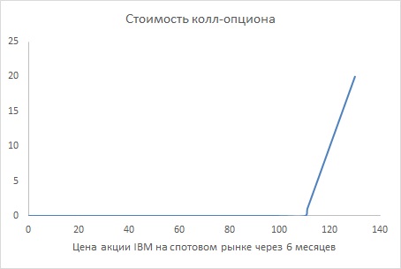
Рис. 1. Стоимость колл-опциона
Скачать заметку в формате Word или pdf, примеры в формате Excel
Основные сведения об опционах
Колл-опцион дает владельцу опциона право купить акцию (или иной актив, например, валюту) по цене исполнения. Пут-опцион дает владельцу опциона право продать акцию по цене исполнения.
Американский опцион может быть исполнен не позднее даты, известной как дата исполнения (часто называемой датой истечения срока действия опциона). Европейский опцион может быть исполнен только в последний день срока его действия.
Давайте рассмотрим итоги сделки по приобретению шестимесячного европейского колл-опциона на акции IBM с ценой исполнения 110 долларов. Пусть P — это курс акции IBM через шесть месяцев. Выигрыш от колл-опциона на эти акции составит 0 долларов, если P < 110 (зачем исполнять опцион, если цена акций на спотовом рынке ниже цены исполнения!?), и (P – 110) долларов, если P > 110. Если значение P больше 110 долларов, владелец может исполнить опцион, купив акцию за 110 долларов и немедленно продав ее на спотовом рынке за P долларов, и тем самым получить прибыль (P – 110) долларов. На рис. 1 представлен выигрыш по этому колл-опциону. Выигрыш можно записать как формулу в Excel =МАКС(0;Р-110). Если Р ≤ 110, говорят опцион не в деньгах.
Ситуация с пут-опциона противоположна (рис. 2). Выигрыш по пут-опциону составит 0 долларов, если P > 110, и (110 – Р) долларов, если P < 110. Для значений P меньше 110 долларов владелец опциона может купить акцию за P долларов и немедленно продать ее за 110 долларов, реализуя опцион. Это принесет прибыль (110 – P) долларов. Если P больше 110 долларов, покупать акцию за P долларов и продавать за 110 долларов невыгодно, так что владелец не исполнит пут-опцион. Формула выигрыша =МАКС(0;110-Р).
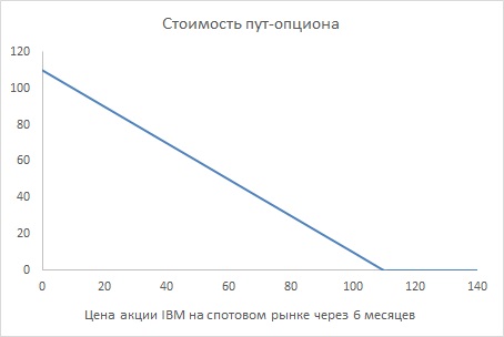
Рис. 2. Стоимость пут-опциона
Параметры, определяющие цену опциона
При создании модели ценообразования Блэк, Шоулз и Мертон показали, что цена опциона зависит от следующих параметров:
- Текущая цена акции (или иного актива).
- Цена исполнения опциона.
- Время (в годах) до истечения срока действия опциона (называемое сроком опциона).
- Процентная ставка (в год с учетом сложных процентов) на безрисковые инвестиции (как правило, в казначейские векселя) в течение всего срока инвестирования. Например, если трехмесячные казначейские векселя приносят 5% дохода, безрисковая ставка вычисляется как ln(1 + 0,05). (Взятие логарифма преобразует простую процентную ставку в ставку с учетом сложных процентов.) Сложные проценты означают, что в каждый момент времени проценты приносят проценты.
- Годовая ставка (в процентах от курса акции), по которой выплачиваются дивиденды. Если акция приносит каждый год 2% своей стоимости в качестве дивидендов, норма дивидендов составляет 0,02.
- Волатильность акции (измеряемая в годовом исчислении). Годовая волатильность акции, например, 30% означает, что (приближенно) стандартное отклонение относительного годичного изменения курса акции составит примерно 30%. Во времена интернет-пузыря в конце 1990-х годов волатильность акций многих интернет-компаний превышала 100%. Этот важный параметр можно вычислить двумя способами.
В формуле ценообразования Блэка–Шоулза курс акции должен соответствовать логарифмически нормальному распределению.
Оценка волатильности акции на основе исторических данных
Для оценки исторической волатильности акции необходимо выполнить следующие шаги:
- Определить прибыль (убыток) по акции за несколько лет.
- Определить для каждого месяца ln(1 + прибыль).
- Определить стандартное отклонение для ln(1 + прибыль). Это вычисление дает ежемесячную волатильность.
- Умножить ежемесячную волатильность на для преобразования ежемесячной волатильности в годовую.
На рис. 3 приведены данные ежемесячной стоимости акций компании Dell за период с августа 1988 г. по май 2001 г. Прибыль равна разности цен за две соседние даты. Ежемесячная волатильность в ячейке Н3 определена по формуле =СТАНДОТКЛОН.В(E2:E155). (Если вам интересно в чем различие между двумя формулами Excel: СТАНДОТКЛОН.В и СТАНДОТКЛОН.Г, см. здесь.) В ячейке Н4 используется формула =КОРЕНЬ(12)*H3. Годовая волатильность акций Dell составляет 57,8%.
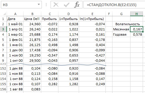
Рис. 3. Вычисление исторической волатильности стоимости акций Dell
Формулу Блэка–Шоулза в Excel
Цена европейского колл-опциона вычисляется по формуле:
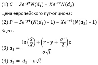
N(x) — вероятность того, что нормальная случайная величина со средним значением 0 и стандартным отклонением σ=1, меньше или равна x. Например, N(-1) = 0,16, N(0) = 0,5, N(1) = 0,84 и N(1,96) = 0,975. Нормальная случайная величина со средним значением 0 и стандартным отклонением 1 называется нормированной случайной величиной, распределенной по нормальному закону. Нормальное интегральное распределение в Microsoft Excel вычисляет функция НОРМ.СТ.РАСП. Формула =НОРМ.СТ.РАСП(x;ИСТИНА) возвращает вероятность того, что нормированная случайная величина, распределенная по нормальному закону, меньше или равна х. Например, формула =НОРМ.СТ.РАСП(-1;ИСТИНА), дает в результате 0,16. Это значение показывает, что нормальная случайная величина со средним значением 0 и стандартным отклонением 1 с вероятностью 16% примет значение менее -1.
S — текущий курс акции; t — срок опциона (в годах); X — цена исполнения; r — годовая безрисковая ставка (предполагается, что эта ставка постоянно вычисляется с учетом сложных процентов); σ — годовая волатильность акции; y — процент от стоимости акции, выплачиваемый в качестве дивидендов.
На рис. 4 находится шаблон, который вычисляет цену для европейских колл- и пут-опционов. Введите значения параметров в ячейки С5:С10 и получите цену европейского колл-опциона в С13, а цену европейского пут-опциона в С14. В качестве примера предположим, что акция Cisco сегодня продается за 20 долларов и вы выпустили семилетний европейский колл-опцион. Пусть годовая волатильность акции Cisco равна 50%, и безрисковая ставка в течение семилетнего периода исчисляется исходя из 5% в год. С учетом сложных процентов она преобразуется в ln(1+0,05) = 0,0488. Компания Cisco не выплачивает дивиденды, так что годовая норма дивидендов равна 0. Цена колл-опциона составляет 10,64 долл. Семилетний пут-опцион с ценой исполнения 24 доллара будет стоить 7,69 долларов.
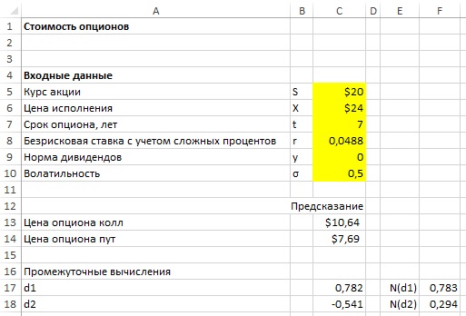
Рис. 4. Определение цены европейских колл- и пут-опционов
Чувствительность стоимости опционов к росту основных параметров
Как правило, влияние изменения входных параметра на цену колл- или пут- опциона соответствует указанному на рис. 5.
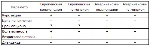
Рис. 5. Влияние роста входных параметров на стоимость опционов
Повышение сегодняшнего курса акции всегда повышает цену колл-опциона и снижает цену пут-опциона.
Повышение цены исполнения всегда повышает цену пут-опциона и снижает цену колл-опциона.
Увеличение срока опциона всегда повышает цену американского опциона. В случае выплаты дивидендов увеличение срока опциона может или повысить, или понизить цену европейского опциона.
Увеличение волатильности всегда повышает цену опциона.
Повышение безрисковой ставки повышает цену колл-опциона, поскольку более высокие ставки имеют тенденцию к увеличению темпов роста курса акции (что хорошо для колл-опциона). Эта ситуация отменяет тот факт, что в результате более высокой процентной ставки выигрыш по опциону уменьшается. Повышение безрисковой ставки всегда понижает цену пут-опциона, поскольку более высокие темпы роста курса акции, как правило, наносят ущерб пут-опциону, и будущий выигрыш по пут-опциону уменьшается. Как и в предыдущем случае, при этом предполагается, что процентные ставки не влияют на текущие курсы акций, однако это не так.
Дивиденды, как правило, снижают темпы роста курса акции, поэтому увеличенные дивиденды снижают цену колл-опциона и повышают цену пут-опциона.
Конкретное влияние изменения параметров на цену колл- и пут-опционов можно исследовать с помощью таблицы данных (рис. 6), см. также Анализ чувствительности в Excel (анализ «что–если», таблицы данных).
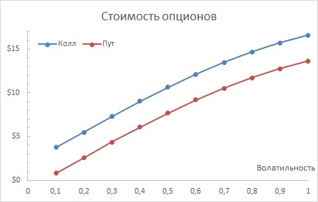
Рис. 6. Анализ чувствительности опционов от волатильности
Оценка волатильности акции по формуле Блэка–Шоулза
Выше было показано, как на основе исторических данных оценить годовую волатильность акций. Проблема с оценкой исторической волатильности состоит в том, что анализ выполняется на основе прошлого. А в действительности требуется оценить волатильность акций на основе ожиданий. Подход на основе подразумеваемой волатильности просто оценивает волатильность акции как значение волатильности, при котором цена по формуле Блэка–Шоулза соответствует рыночной цене опциона. Иными словами, подразумеваемая волатильность получает значение волатильности, вытекающее из рыночной цены опциона.
Для вычисления подразумеваемой волатильности можно воспользоваться инструментом Подбор параметра и описанными ранее входными параметрами (см. рис. 4). 22 июля 2003 г. акция Cisco продавалась за 18,43 долларов. В октябре 2003 г. колл-опцион с ценой исполнения 17,50 долларов продавался за 1,85 долларов. Срок действия этого опциона истекал 18 октября (через 89 дней в будущем). Таким образом, срок действия опциона составляет 89/365 = 0,2438 лет. Предположительно, Cisco не выплачивает дивиденды. Пусть ставка для казначейских векселей составляет 5%, и соответствующая безрисковая ставка равна ln(1 + 0,05) = 0,04879. Для определения волатильности акции Cisco, которая подразумевается ценой опциона, введите в ячейки B5:B10 (рис. 7) релевантные параметры.
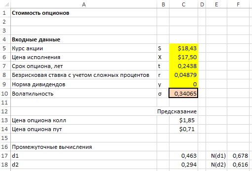
Рис. 7. Вычисление волатильности акции Cisco согласно подразумеваемой волатильности
Далее в диалоговом окне Подбор параметра (Меню Данные –> Анализ «что-если»), показанном на рис. 8, определите волатильность (значение в ячейке B10), при которой цена опциона (формула в С13) достигает значения 1,85 долларов.
Как показано на рис. 7, этот опцион подразумевает годовую волатильность для Cisco в размере 34%.
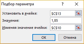
Рис. 8. Настройки в диалоговом окне Подбор параметра
На сайте http://www.ivolatility.com/ и http://www.ivolatility.ru/ предоставляются оценки волатильности любой акции, как исторические, так и подразумеваемые.
Реальные опционы
Ценообразование опционов может повлиять на повышение эффективности долгосрочных инвестиций компании или на процесс принятия финансовых решений. Использование ценообразования опционов для оценки фактических инвестиционных проектов называется реальными опционами. Идею реальных опционов приписывают Джуди Левен, в прошлом финансовому директору компании Merck. По существу, реальные опционы позволяют назначить явную цену для управленческой гибкости, которую часто упускают из вида при традиционном составлении плана долгосрочных инвестиций. Рассмотрим два примера.
Пусть вы являетесь владельцем нефтяной скважины. Сегодня наиболее правдоподобное предположение о стоимости нефти в скважине — 50 млн. долларов. Через 5 лет (оставаясь владельцем скважины) вам предстоит принять решение о разработке нефтяной скважины, которая обойдется вам в 70 млн. долларов. Бизнесмен с сомнительной репутацией готов купить скважину сегодня за 10 млн. долларов. Следует ли продать скважину?
Безусловно, цена нефти через 5 лет может вырасти. Даже если предположить, что цена нефти будет расти на 5% в год, через 5 лет нефть будет стоить 63,81 млн долларов. Традиционный план долгосрочного инвестирования предполагает, что нефть обесценится, поскольку стоимость ее разработки превышает стоимость нефти в скважине. Но не торопитесь — через 5 лет цена нефти в скважине будет другой, т.к. многие вещи (такие как мировая цена на нефть) могут измениться. Существует вероятность, что через 5 лет нефть будет стоить не меньше 70 млн. долларов. Если через 5 лет нефть будет стоить 80 млн. долларов, разработка скважины через пять лет принесет 10 млн долларов.
По сути, вы владеете пятилетним европейским колл-опционом на эту скважину, т.к. выигрыш от скважины через 5 лет такой же, как выигрыш по европейскому колл-опциону с курсом акции 50 млн. долларов, ценой исполнения 70 млн. долларов и сроком опциона 5 лет. Можно предположить, что годовая волатильность подобна волатильности акции типичной нефтяной компании (например, 30%). Если использовать безрисковую ставку 4,879%, можно определить, что цена такого колл- опциона составляет 11,47 млн. долларов (рис. 9). Из этого следует, что вы не должны продавать скважину за 10 млн. долларов.
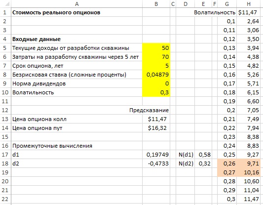
Рис. 9. Реальный опцион на нефтяную скважину
Конечно, фактическая волатильность для этой нефтяной скважины неизвестна. По этой причине с помощью таблицы данных с одним входом определим, как цена опциона зависит от оценки волатильности (см. рис. 9). Как видно из таблицы, пока волатильность скважины составляет, по меньшей мере, 27%, опцион на нефтяную скважину стоит более 10 млн. долларов.
В качестве второго примера рассмотрим биотехнологическую компанию по производству лекарств, разрабатывающую лекарственный препарат для фармацевтической фирмы. В биотехнологической компании в настоящее время предполагают, что цена разрабатываемого препарата составляет 50 млн. долларов. Безусловно, цена лекарственного препарата со временем может понизиться. Для защиты от резкого падения цены биотехнологической компании требуется, чтобы препарат через 5 лет имел гарантированную цену 50 млн. долларов. Если страховая компания собирается подписать такое обязательство, какая справедливая цена должна быть назначена?
По существу, биотехнологическая компания запрашивает платеж в 1 млн. долларов для каждого миллиона долларов, на который цена препарата упадет ниже уровня 50 млн. долларов, через 5 лет. Это эквивалентно пятилетнему пут-опциону на цену лекарственного препарата. Предположим, что ставка по казначейскому векселю составляет 5% и годовая волатильность для акций сопоставимых компаний равна 40% (рис. 10), тогда цена этого опциона — 10,51 млн. долларов. Такой тип опциона часто называют опционом на отказ от проекта, но он эквивалентен пут-опциону. (На рис. 10 таблица данных показывает, как цена опциона отказа от проекта зависит от предполагаемой волатильности, составляющей 30–45% от цены лекарственного препарата.)

Рис. 10. Вычисление стоимости пут-опциона отказа от проекта
[1] Заметка написана на основе материалов из книги Уэйн Л. Винстон. Microsoft Excel 2013. Анализ данных и бизнес-моделирование, глава 78.
This page is a guide to creating your own option pricing Excel spreadsheet, in line with the Black-Scholes model (extended for dividends by Merton). Here you can get a ready-made Black-Scholes Excel calculator with charts and additional features such as parameter calculations and simulations.
Black-Scholes in Excel: The Big Picture
If you are not familiar with the Black-Scholes model, its assumptions, parameters, and (at least the logic of) the formulas, you may want to read those pages first (overview of all Black-Scholes resources is here).
Below I will show you how to apply the Black-Scholes formulas in Excel and how to put them all together in a simple option pricing spreadsheet. There are four steps:
- Design cells where you will enter parameters.
- Calculate d1 and d2.
- Calculate call and put option prices.
- Calculate option Greeks.
Black-Scholes Inputs

First you need to design six cells for the six Black-Scholes parameters. When pricing a particular option, you will have to enter all the parameters in these cells in the correct format. The parameters and formats are:
S = underlying price (USD per share)
K = strike price (USD per share)
σ = volatility (% p.a.)
r = continuously compounded risk-free interest rate (% p.a.)
q = continuously compounded dividend yield (% p.a.)
t = time to expiration (% of year)
Underlying price is the price at which the underlying security is trading on the market at the moment you are doing the option pricing. Enter it in dollars (or euros/yen/pound etc.) per share.
Strike price, also called exercise price, is the price at which you will buy (if call) or sell (if put) the underlying security if you choose to exercise the option. If you need more explanation, see: Strike vs. Market Price vs. Underlying Price. Enter it also in dollars per share (it must have same units as underlying price, also with the same contract or lot multipliers).
Volatility is the most difficult parameter to estimate (all the other parameters are more or less given). It is your job to decide how high volatility you expect and what number to enter – neither the Black-Scholes model, nor this page will tell you how high volatility to expect with your particular option (for more on that, see the volatility tutorials, particularly historical and implied volatility). Being able to estimate (= predict) volatility with more success than other people is the hard part and key factor determining success or failure in option trading. The important thing here is to enter it in the correct format, which is % p.a. (percent annualized).
Risk-free interest rate should be entered in % p.a., continuously compounded. The interest rate’s tenor (time to maturity) should match the time to expiration of the option you are pricing. You can interpolate the yield curve to get the interest rate for your exact time to expiration. Interest rate does not affect the resulting option price very much in the low interest environment that we’ve had in the recent years, but it can become very important when rates are higher (for more details on the effect of interest rates on option prices see the option rho tutorial).
Dividend yield should also be entered in % p.a., continuously compounded. If the underlying stock doesn’t pay any dividend, enter zero. If you are pricing an option on securities other than stocks, you may enter the second country interest rate (for FX options) or convenience yield (for commodities) here.
Time to expiration should be entered as % of year between the moment of pricing (now) and expiration of the option. For example, if the option expires in 24 calendar days, enter 24/365 = 6.58%. Alternatively, you can measure time in trading days rather than calendar days. If the option expires in 18 trading days and there are 252 trading days per year, you will enter time to expiration as 18/252 = 7.14%. You can also be more precise and measure time to expiration to hours or even minutes. In any case you must always express the time to expiration as % of year in order for the calculations to return correct results (it is very easy in Excel – just divide the number of days to expiration by the number of days per year).
I will illustrate the calculations on the example below. The parameters are in cells A44 (underlying price), B44 (strike price), C44 (volatility), D44 (interest rate), E44 (dividend yield), and G44 (time to expiration as % of year).

Note: It is row 44, because I am using the Black-Scholes Calculator for screenshots and it has charts in the rows above. You can of course start in row 1 or arrange your calculations in a column.
Black-Scholes d1 and d2
When you have the cells with parameters ready, the next step is to calculate d1 and d2, because these terms then enter all the calculations of call and put option prices and Greeks. The formulas for d1 and d2 are:


All the operations in these formulas are relatively simple mathematics. The only things that may be unfamiliar to some less savvy Excel users are the natural logarithm (LN Excel function) and square root (SQRT Excel function).
The hardest thing with the d1 formula is making sure you put the brackets in the right places. This is why you may want to calculate individual parts of the formula in separate cells, as I do in the example below:

First I calculate the natural logarithm of the ratio of underlying price and strike price (this is why they must have the same units) in cell H44:
=LN(A44/B44)
Then I calculate the rest of the numerator of the d1 formula in cell I44:
=(D44-E44+POWER(C44,2)/2)*G44
Then I calculate the denominator of the d1 formula in cell J44. Another reason why you may want to calculate d1 in separate parts is that this term will also enter the formula for d2:
=C44*SQRT(G44)
Now I have all the three parts of the d1 formula and I can combine them in cell K44 to get d1:
=(H44+I44)/J44
Finally, I calculate d2 in cell L44:
=K44-J44
Black-Scholes Option Price Excel Formulas
The Black-Scholes formulas for call option (C) and put option (P) prices are:


The two formulas are very similar. There are four terms in each formula. I will again calculate them in separate cells first and then combine them in the final call and put formulas.
N(d1), N(d2), N(-d2), N(-d1)
Potentially unfamiliar parts of the formulas are the N(d1), N(d2), N(-d2), and N(-d1) terms.
N(x) denotes the standard normal cumulative distribution function:
")
For example, N(d1) is the standard normal cumulative distribution function for the d1 that we have calculated in the previous step.
In Excel you can easily calculate the standard normal cumulative distribution functions using the NORM.DIST function, which has four parameters:
NORM.DIST(x, mean, standard_dev, cumulative)- x = link to the cell where you have calculated d1 or d2 (with minus sign for -d1 and -d2)
- mean = enter 0, because it is standard normal distribution
- standard_dev = enter 1, because it is standard normal distribution
- cumulative = enter TRUE, because it is cumulative
For example, I calculate N(d1) in cell M44:
=NORM.DIST(K44,0,1,TRUE)
Note: There is also the NORM.S.DIST function in Excel, which is the same as NORM.DIST with fixed mean = 0 and standard_dev = 1 (therefore you enter only two parameters: x and cumulative). You can use either. NORM.S.DIST may not be available in some spreadsheet software.
The Terms with Exponential Functions
The exponents (e-qt and e-rt terms) are calculated using the EXP Excel function with -q*t or -r*t as parameter.
I calculate e-rt in cell Q44:
=EXP(-D44*G44)
Then I use it to calculate K e-rt in cell R44:
=B44*Q44
Analogically, I calculate e-qt in cell S44:
=EXP(-E44*G44)
Then I use it to calculate S e-qt in cell T44:
=A44*S44
Now I have all the individual terms and I can calculate the final call and put option price.
Call Option Price
I combine the four terms in the call formula to get call option price in cell U44:
=T44*M44-R44*O44
Put Option Price
I combine the four terms in the put formula to get put option price in cell U44:
=R44*P44-T44*N44
Black-Scholes Greeks in Excel

Here you can continue to the second part of this tutorial, which explains Excel calculation of the Greeks: delta, gamma, theta, vega, and rho:
Continue to Option Greeks Excel Formulas
Or you can see how all the Excel calculations work together in the Black-Scholes Calculator. Explanation of the calculator’s other features (parameter calculations and simulations of option prices and Greeks) are available in the calculator’s user guide.
Содержание
- How to calculate Option Pricing using Monte Carlo Simulations in Excel
- Monte Carlo Simulation
- European-style Options Pricing
- Calculating Option Pricing with VBA
- Black-Scholes option pricing in Excel and VBA
- 1. Black-Scholes model
- 2. The Black-Scholes model in Excel
- 3. The Black-Scholes model in VBA
- References
- Related material
- Binomial Option Pricing Excel Tutorial
- Required Excel Skills
- Let’s Start: Preparing Input Cells
- Naming the Input Cells
- Next: Binomial Trees
- Options Pricing & Valuation models Start the discussion!
- What is an Option?
- Call Option vs. Put Option
- Option Pricing Models
How to calculate Option Pricing using Monte Carlo Simulations in Excel
In finance, option pricing is a term used for estimating the value of an option contract using all known inputs. Monte Carlo Simulation is a popular algorithm that can generate a series of random variables with similar properties to simulate realistic inputs. In this guide, we’re going to show you how to calculate Option Pricing using Monte Carlo Simulations in Excel.
Monte Carlo Simulation
Monte Carlo simulation is a special type of probability simulation which is mainly used to determine the risk factors by observing the cluster of possible results. First developed for finding the possible outcomes of a solitaire game, Monte Carlo takes its name from the famous casino in Monaco.
The simulation takes random values of the inputs within constraints and the results are recorded as more iterations are run. Then, you get a rather big pool of answers created from all those random inputs.
We can simulate the possible future stock prices and then use them to find the discounted expected option payoffs.
Using the statistical formulas NORM.S.INV and VBA, we can generate random variables in normal distribution and run the simulation as many times as necessary..
European-style Options Pricing
In this example, we are going to be using the Black-Scholes formula to calculate a European-style option pricing model, which restricts its options execution until the expiration date. There are two major types of options: calls and puts.
- Call is an option contract between the buyer and the seller of the call option, to exchange a security at a set price.
- Put is an option contract which gives the purchaser of the put option the right to sell an asset, at a specified price, by a specified date to the seller of the put.
The Black-Scholes formula is a popular approach for calculating European put and call options. In its simplest form, the Black-Scholes model involves underlying assets of a risk-free rate of return and a risky share price. The following equation shows how a stock price varies over time:

St = Stock price at time t
r = Risk-free rate
σ = T he volatility of the stock’s returns; this is the square root of the quadratic variation of the stock’s log price process
ε = random generated variable from a normal distribution
δ = Dividend yield which was not in the Black-Scholes model originally. The original model was for pricing options on non-paying dividends stocks.
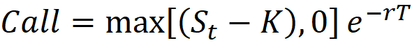
Once the formula is run thousands or million times, you will have the set of St values. The payoff values can be calculated with the following formula, where K is the strike price:

Calculating Option Pricing with VBA
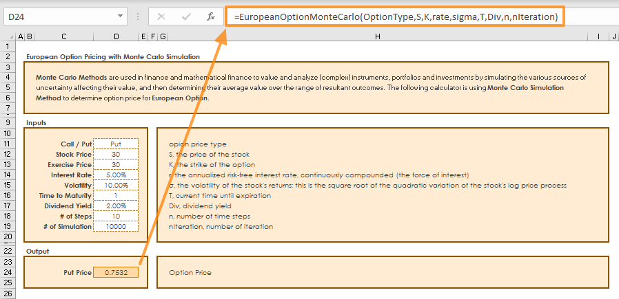
Let’s pass these formulations into a VBA code. We are going to create a user defined function (UDF) which can be used as a built-in function like SUM or VLOOKUP. Our function name is “EuropeanOptionMonteCarlo”.
Once the UDF is ready, we are ready to see the result in Excel.
Источник
Black-Scholes option pricing in Excel and VBA
1. Black-Scholes model
According to the Black-Scholes (1973) model, the theoretical price (C) for European call option on a non dividend paying stock is $$begin C=S_0 N(d_1)-Xe^<-rT>N(d_2) end$$ where $$d_1=frac right) + left( r+ frac <sigma^2> <2>right )T><sigma sqrt> $$ $$d_2=frac right) + left( r — frac <sigma^2> <2>right )T><sigma sqrt> = d_1 — sigma sqrt$$
In equation 1, (S_0) is the stock price at time 0, (X) is the exercise price of the option, (r) is the risk free interest rate, (sigma) represents the annual volatility of the underlying asset, and (T) is the time to expiration of the option.
From Put-Call parity, the theoretical price (P) of European put option on a non dividend paying stock is $$begin P=Xe^<-rT>N(-d_2) — S_0 N(-d_1) end$$
2. The Black-Scholes model in Excel
Example: The stock price at time 0, six months before expiration date of the option is $42.00, option exercise price is $40.00, the rate of interest on a government bond with 6 months to expiration is 5%, and the annual volatility of the underlying stock is 20%.
The values used in this example are similar to those in Hull (2009, p294 ) with S0 = 42, K (exercise) = 40, r = 0.1, σ = 0.2, and T = 0.5. This set returns c = 4.76 and p = 0.81
Calculation of the call price can be completed as a 5 step process. Step 1. d1; 2. d2 as ( left[frac right) + left( r — frac <sigma^2> <2>right )T><sigma sqrt> right]); 3. N(d1); 4. N(d2); and step 5, C. The value for d1 and d2 are shown in rows 12 and 13 of figure 1. The probabilities for (N(cdot)) are estimated with the NORM.S.DIST function. The call price from equation 1 is $4.08 (Figure 1 row 18), and the put price from equation 2 is $1.09 (Figure 1 row 19).
Syntax NORM.S.DIST(z,cumulative) . z is the probability value, and cumulative is a LOGICAL value. TRUE returns the cumulative distribution function. FALSE returns the probability mass function.
Fig 1: Excel Web App #1: — Excel version of Black and Scholes’ model for a European type option on a non dividend paying stock
3. The Black-Scholes model in VBA
In this example, separate function procedures are developed for the call (code 1) and put (code 2) equations. The Excel NORM.S.DIST function, line 6 in code 1 and 2, requires that the dot operators be replaced by underscores when the function is called from VBA.
The BScall and BSPut functions are tested by the calling procedure in code 3. Output is sent to the Immediate Window with the Debug.Print method.
The output from code 3 is shown in the Immediate Window of figure 2.
 Fig 2: Black and Scholes’ model — for a European type option on a non dividend paying stock
A combination Call and Put procedure is shown in Code 4.
The BSOption function functions is tested by the calling procedure in code 5.
References
Black F, and M Scholes, (1973), The pricing of options and corporate liabilities, Journal of Political Economy, Vol 81 No 3 pp.637-654.
Hull J, (2009), ‘Options, futures, and other derivatives’, 7th ed., Pearson Prentice Hall
Black Scholes on the HP10bII+ financial calculator
Social media links
Added 24th February 2016
- Download the Excel file for this module: bs_nondiv.xlsm [29 KB]
- Download the VBA code for this module: xlf-black-scholes-code.txt [4 KB]
- Development platform: Microsoft Excel 2013 Pro 64 bit.
- Revised: Friday 24th of February 2023 — 10:37 PM, Pacific Time (PT)
Copyright © 2011 – 2023 ♦ Dr Ian O’Connor, CPA. | Privacy policy
Источник
Binomial Option Pricing Excel Tutorial
Binomial Option Pricing Excel Tutorial:
Binomial Model Formulas and Reference:
In this tutorial we will create an option pricing spreadsheet, implementing three popular binomial models: Cox-Ross-Rubinstein, Jarrow-Rudd and Leisen-Reimer.
The spreadsheet will calculate prices of American and European options on stocks, indexes and currencies.
The tutorial has six parts:
If you are already familiar with binomial models and how binomial trees work, you can safely skip part 2.
If not, you will be able to complete the tutorial even if you know nothing about binomial models at the moment. In fact, this hands-on approach is the best way to learn them.
If you are only interested in one of the models, you can skip the parts for the other two models (part 4/5/6).
All three models share the same logic and most of the work is exactly the same (preparing input cells, building binomial trees – covered in parts 1-3). The only part where the models differ is the exact formulas for binomial tree up and down move sizes and probabilities (parts 4/5/6 for individual models).
Required Excel Skills
You don’t need advanced Excel skills to complete this tutorial. You should be comfortable with basic concepts like writing and copying formulas or absolute and relative references.
The hard part of binomial models is the logic and layout of binomial trees; the mathematics is relatively simple. The Excel functions we will use are mostly basic, like SQRT , EXP , and a lot of IF s.
This tutorial will not use VBA and macros.
Let’s Start: Preparing Input Cells
To calculate option prices with binomial models you need a number of inputs, like underlying price, strike price, time to expiration, volatility or interest rate. If you know the Black-Scholes model, you will find the inputs are the same.
It is best to prepare cells for all the inputs right at the beginning, and have all the input cells in one place. It will make the spreadsheet easier to use.
Let’s put our inputs in cells B4-B11 and their labels in column A .
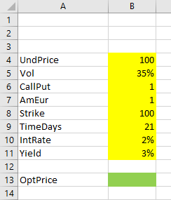
- UndPrice = current underlying price
- Vol = volatility
- CallPut = whether the option is a call (1) or put (2)
- AmEur = whether the option is American (1) or European (2)
- Strike = the option’s strike price
- TimeDays = time to expiration as number of days; fractional days will also work
- IntRate = the risk-free interest rate (domestic rate for currency options)
- Yield = continuous dividend yield (for stocks, indexes) or foreign rate (for currency options)
For detailed explanation and which values to use, see Binomial Option Pricing Model Inputs.
The output which we want to calculate is the option price ( OptPrice ) in cell B13 .
As in other tutorials and calculators, I use yellow background for input cells and green background for output cells.
Note: If you know how to create combo boxes, you can use them for the CallPut , AmEur inputs. Just make sure call is 1, put is 2, and American is 1, European is 2.
Naming the Input Cells
To make our formulas easier to write, understand and debug, it is best to name our input cells. It will allow use to write formulas like:
This is how to make it work:
First, make sure your labels in cells A4-A11 are exactly like mine ( UndPrice , Vol etc.).
Select all the input cells and their labels (the selection is A4-B11 ).
In Excel main menu, go to «Formulas» / «Defined Names» section and click on «Create from Selection».
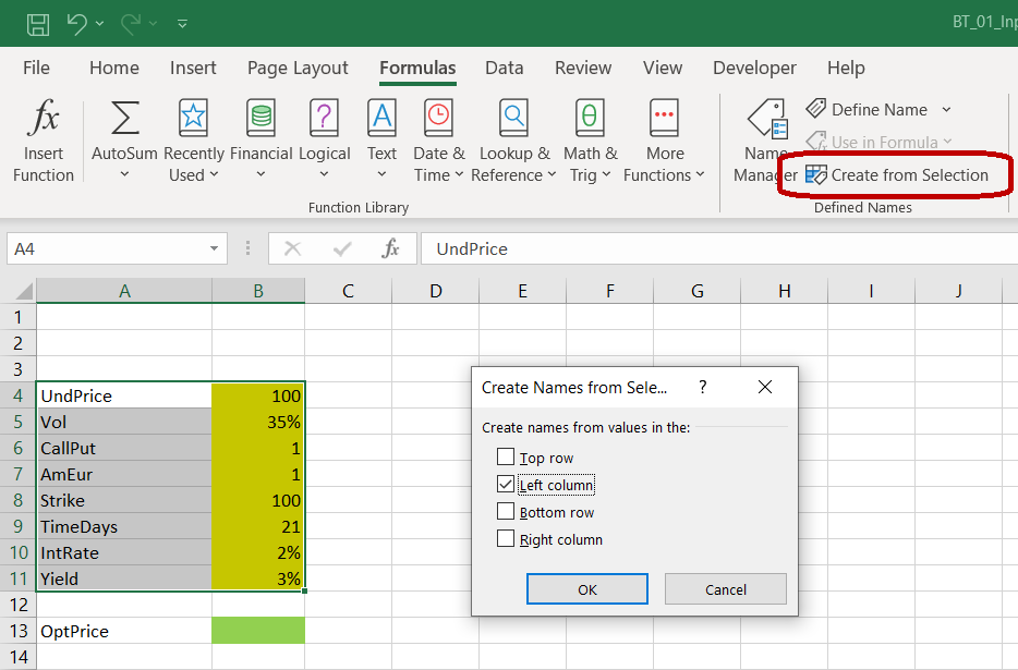
In the window that pops up, check «Left column». This tells Excel to use the contents in the left column (the labels in column A ) as names for the cells in the right column (the input values in column B ). Click OK.
Now when you select cell B4 for instance, the small window on the left of the formula bar is showing «UndPrice» instead of «B4».
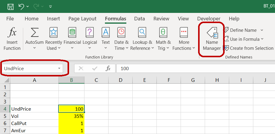
In formulas, you can now refer to the cell as UndPrice instead of $B$4 .
1) You can also set or change cell names one by one by overwriting the text in the cell name window or by using Name Manager (as highlighted in the screenshot above).
2) The navigation may be different in other Excel versions. If you can’t find it in yours, google «how to name cells in excel [your version]».
Next: Binomial Trees
We have our inputs ready and can start working on the calculations. The central part of any binomial option pricing model is the binomial tree, or more precisely, two trees – underlying price tree and option price tree.
In the next part, we will explain how they work (safe to skip if you already know that).
In the part that follows, we will actually create them in our spreadsheet.
Источник
Options Pricing & Valuation models Start the discussion!

What is an Option?
• An option is a financial derivative which means it derives its value from another financial security. An option writer sells the option to an option buyer. The agreed-on price between the two parties is called the strike price and there is always a specified date which signifies when the option expires. You can exercise your right to buy or sell the option. This means you do not have to buy or sell if you do not want to. If you hold an American option, then you can exercise your right on the option any time before the expiration date. If you hold a European option, you can only exercise your right on the expiration date. They are mainly used to speculate or hedge any of your current holdings.
Call Option vs. Put Option
• A call option allows the buyer to buy the underlying security at the strike price. In this situation, the buyer would want the price of the stock to be higher than the strike price because the buyer pays the agreed upon strike price. This allows the buyer to sell the stock at the current market price and make a profit from it. If you write a call option, you believe that the price of the stock will either drop or stay the same. The profit that a writer can make from selling a call option is the difference between the price of the stock and the strike price, the premium.
• A put option allows the buyer of the option to sell the underlying security at the strike price. A buyer of a put option wants the price of the security to drop because the buyer can sell the security at a strike price that is higher than the market price. However, a put option writer wants the price of the security to raise above the strike price because the buyer would have to sell it to them at a lower price.
Option Pricing Models
• Two ways to price options are the Black-Scholes model and the Binomial model. The Black-Scholes model is used to find to find a call price by using the current stock price, strike price, the volatility, risk free interest rate, and the time until the option expires. The Binomial model uses a tree of stock prices that is broken down into intervals. This tree represents the potential value of a stock from the present date and until the expiration. From this, one can find the value of the option with the strike price, volatility, risk free interest rate and the stock price at expiration date.
Источник
- Finance
- Accounting
- Amortization & Depreciation Schedule
- Balance Sheet
- Bank Financial Models
- Black-Scholes Models
- Capital Budgeting
- Cash Flow Statement
- Corporate Finance
- Cost Analysis
- Debt Schedule
- Discounted Cash Flow (DCF)
- Excel
- Excel Add-Ins
- Excel VBA
- Financial Forecasting Models
- Financial Markets
- Financial Modeling
- Financial Projections Models
- Income Statement
- Industry Specific Financial Models
- Inventory Management
- Investment Banking
- Leveraged Buyout (LBO)
- Mergers & Acquisitions (M&A)
- ModelOff Samples
- Monte Carlo Simulation
- Net Present Value (NPV)
- Options Pricing & Valuation
- Private Equity
- Project Finance Models
- Real Estate Financials
- Renewable Energy Financials
- Restaurant Finance
- Retail Finance
- Return On Investment (ROI)
- Scenario Analysis
- Sensitivity Analysis
- Solar Energy Project Finance
- Stock Valuation
- Three Statement Financial Models
- Trading
- Valuation Models
- Venture Capital
- Weighted Average Cost Of Capital (WACC)
- Wind Energy Project Finance
listView all 92 sub-categories
- Strategy
- 2×2 Four Quadrant Matrix
- Ansoff Matrix
- Asset Management
- Balanced Scorecard
- BCG Frameworks
- BCG Growth-Share Matrix
- Business Development
- Business Model Canvas —
- Business Plans
- Change Management
- Coaching
- Competitor Analysis
- Consulting Interview
- Consulting Proposals
- Crisis Management
- Due Diligence
- Executive Summary
- Heat Maps
- KPI Dashboards
- Logistics & Supply Chain Management
- Macroeconomics
- Management Consulting
- Market Analysis
- Market Research
- Market Sizing
- McKinsey 7-S Framework
- McKinsey Frameworks
- Microeconomics Excel
- Mission Statement
- Nine-Box Matrix
- Operations Management
- Porter’s Five Forces
- Post-Merger Integration (PMI)
- Problem Solving
- Roadmaps
- Sales
- SMART Goals
- Strategic Analysis
- Strategic Management
- Strategic Partnerships
- Strategic Planning
- SWOT Analysis
- Value Chain Analysis
- Value Creation
- Waterfall Charts
listView all 71 sub-categories
- Startups
- Cohort Analysis
- Design Thinking Process
- E-Commerce Financial Models
- Entrepreneurship
- Freemium
- Growth Hacking
- Lean Startup
- Lifetime Value (LTV)
- Marketplaces
- Mobile App Finance
- Raising Capital
- Software-as-a-Service (SaaS)
- Startup Boards
- Startup Business Plans
- Startup Cap Tables
- Startup Financial Models
- Startup Investors
- Startup Lifestyle
- Startup Pitch Decks
- Startup Studios
- Startup Valuation
- Marketing
- 4Ps & 7Ps Marketing Mix
- Advertising
- Branding & Brand Management
- Business Email
- Business Networking
- Corporate Communication
- Customer Acquisition
- Customer Centric Design
- Customer Success
- Digital Marketing
- Growth Marketing
- Inbound Marketing
- Industry Landscape Analysis
- Lead Generation
- Marketing Plans
- Net Promoter Score (NPS)
- Outbound Sales
- Personal Branding
- Pricing
- Product Launch
- Product Life Cycle
- Public Relations
- Public Speaking
- Search Engine Optimization (SEO)
- Social Media
- Strategic Marketing
- Legal
- Advisor Agreements
- Articles Of Incorporation
- Code Of Conduct
- Compliance
- Employee Contracts
- Intellectual Property (IP) Agreements
- Internal Audit
- Non-Disclosure Agreements
- Operating (or Founder) Agreements
- Sales & Purchase Agreements (SPA)
- Shareholder Agreements
- Startup Term Sheets
- Leadership & HR
- Career Advancement
- Chief Of Staff
- Corporate Event Management
- Cross Cultural Management
- CV (Curriculum Vitae) / Resume
- Decision Making
- Effective Communication
- Gantt Charts
- Health & Safety
- Human Resources
- Interviews
- Job Descriptions
- Job Search
- Leadership
- Meetings
- Organizational Charts
- Organizational Culture
- Payroll
- Performance Reviews & Appraisals
- Personal Development
- Productivity
- Project Management
- Recruiting
- Remote Work
- Task Management
- Team Management
- Teamwork
- Training Excel
- Technology
- Artificial Intelligence (AI)
- Blockchain Technology
- Cryptocurrency
- Cybersecurity
- Data Analysis
- Data Mining
- Data Science
- Digital Privacy
- Electrical Engineering
- Genetic Engineering
- Google Sheets Models
- JavaScript
- Machine Learning
- Mathematical
- Neural Networks
- NFT Investment
- Power BI
- Product Management
- Research And Development (R&D)
- Statistical
- UI Design
- UX Design
- Student
- Dissertation Writing
- Essay Writing
- Exam Revision
- Group Work
- Student Life
- Study Note-Taking
- University Research
- Other
- Coronavirus (COVID-19)
- Dynamic Arrays
- ELearning
- Eloquens Authors
- Miscellaneous
- Politics & Politicians
- All
Options Pricing & Valuation models
Start the discussion!
What is an Option?
• An option is a financial derivative which means it derives its value from another financial security. An option writer sells the option to an option buyer. The agreed-on price between the two parties is called the strike price and there is always a specified date which signifies when the option expires. You can exercise your right to buy or sell the option. This means you do not have to buy or sell if you do not want to. If you hold an American option, then you can exercise your right on the option any time before the expiration date. If you hold a European option, you can only exercise your right on the expiration date. They are mainly used to speculate or hedge any of your current holdings.
Call Option vs. Put Option
• A call option allows the buyer to buy the underlying security at the strike price. In this situation, the buyer would want the price of the stock to be higher than the strike price because the buyer pays the agreed upon strike price. This allows the buyer to sell the stock at the current market price and make a profit from it. If you write a call option, you believe that the price of the stock will either drop or stay the same. The profit that a writer can make from selling a call option is the difference between the price of the stock and the strike price, the premium.
• A put option allows the buyer of the option to sell the underlying security at the strike price. A buyer of a put option wants the price of the security to drop because the buyer can sell the security at a strike price that is higher than the market price. However, a put option writer wants the price of the security to raise above the strike price because the buyer would have to sell it to them at a lower price.
Option Pricing Models
• Two ways to price options are the Black-Scholes model and the Binomial model. The Black-Scholes model is used to find to find a call price by using the current stock price, strike price, the volatility, risk free interest rate, and the time until the option expires. The Binomial model uses a tree of stock prices that is broken down into intervals. This tree represents the potential value of a stock from the present date and until the expiration. From this, one can find the value of the option with the strike price, volatility, risk free interest rate and the stock price at expiration date.
For more information:
Investopedia
How to Trade Options
Option Pricing Models
The Binomial Option Pricing Model Excel is available as a template with MarketXLS. The Binomial Option Pricing Model is a popular model for stock options evaluation, and to calculate the options premium.
The Binomial Options Pricing Model provides investors with a tool to help evaluate stock options. The model uses multiple periods to value the option. For each period, the model simulates the options premium at two possibilities of price movement (up or down). The periods create a binomial tree — In the tree, each tree shows the two possible outcomes or the movement of the price.
The model creates a binomial distribution of possible stock prices for the option. It creates possible paths that the stock price could go until the expiration date and the resulting impact on the options premium. Unlike the Black Scholes model of valuation of the option premium, the Binomial model gives you a view of an option contract at different prices at different periods until the expiration date.
Black-Scholes Vs Binomial Model
Black-Scholes model assumes that the option contract you are pricing is a European style option contract. A European style option contract is the one that can only be exercised at the date of the Expiry. The Americal style options contracts are the ones that can be exercised on any day until the expiry. Unlike, the Black Scholes model the Binomial option pricing model excel calculates the price of the option at various periods until the expiry. Since most of the exchange-traded options are American style options, the Black Scholes model seems to have a limitation.
If you were to assume that each period (days/weeks/months) until the expiry is the expiry date itself, you could also use the Black Scholes model to calculate a similar pay off table showing the value of the option for each period until expiry.
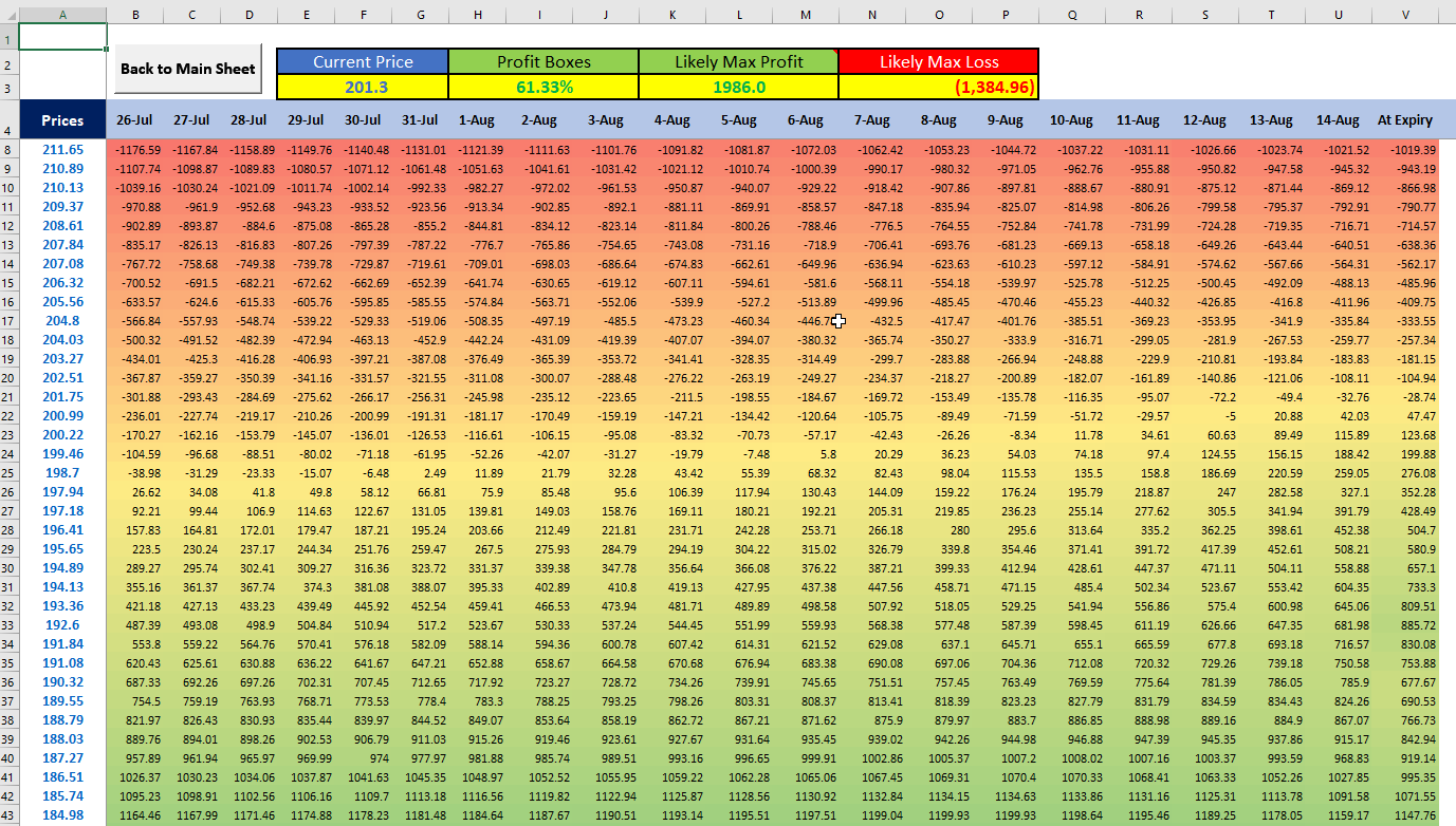
See the example below, where I use the Black Scholes model to generate a payoff for an option contract until the expiry date by assuming each day until the expiry is the expiry date. You can refer to our Options Profit Calculator template here.
How do you calculate the Option Premiums using the Binomial Model?
The Binomial Option Pricing Model Excel takes the following as the Inputs. For example, I have taken a Call Option of American Airlines expiring on August 7th, 2020 and today is 29th of July 2020. So, there are 10 days left until the expiry. The variable T as shown below in the days to expiry and n is the number of steps that we need in our Binomial tree. The current price of this option is 0.54 per contract. And the stock price is at 11.77. The following table shows other values and assumptions.
S = 11.77 #underlying pricek = 12 #Strike pricer = .04 #Riskfree ratev = .81 #VolatilityT = 10./365 #Time to maturityn = 10 #StepsUn= 1 #1 Unit is 100 stocksPC = 0 #Call option
The first step in the calculation is to create a binomial tree. This tree will have a specified amount of time that ends at the expiration date. Each point on the tree is a node. And each node is the price the stock can go at. The following image shows the binomial tree for the stock price movement(in table 1). So, for each period the table below shows the possible price movement on the underlying stock.
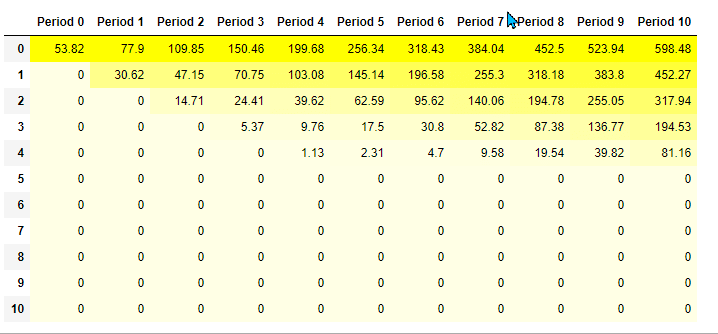
This chart below is the table for the price of the stock and the one below it is the table for the price of the option contract at corresponding prices (in table 2). And finally we have a table that shows the expected payoffs (in dollars) at these prices (in table 3) until the expiry when we buy 1 contract of this call option.
TABLE 1:
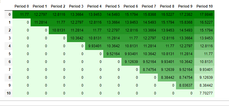
TABLE 2:
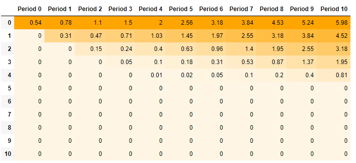
TABLE 3:
The binomial tree diagram represents the option payoff and probability at different nodes. Nodes outline the paths the price of the underlying asset may take over time. The following binomial tree represents the general one-period call option.
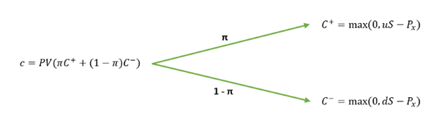
The option value using the one-period binomial option pricing model can be worked out using the following formula:
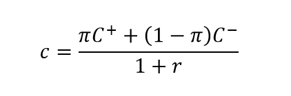
The put option uses the same formula as the call option:
Where:
C+ is the payoff of an up move;
C- is the payoff of the down move;
π is the probability of an up move;
1-π is the probability of the down move;
r is the discount rate.
Where π is the probability of an up move which is determined using the following equation:
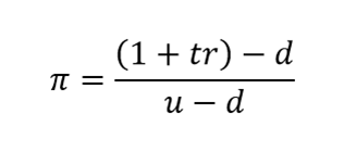
Where:
t is the period multiplier (time to maturity);
r is the discount rate;
d is the down factor;
u is the up factor.
The binomial option pricing model excel is useful for options traders to help estimate the theoretical values of options. Price movements of the underlying stocks provide insight into the values of options premium. The model offers a calculation of what the price of an option contract could be worth today.