
Have you ever used VLOOKUP to bring a column from one table into another table? Now that Excel has a built-in Data Model, VLOOKUP is obsolete. You can create a relationship between two tables of data, based on matching data in each table. Then you can create Power View sheets and build PivotTables and other reports with fields from each table, even when the tables are from different sources. For example, if you have customer sales data, you might want to import and relate time intelligence data to analyze sales patterns by year and month.
All the tables in a workbook are listed in the PivotTable and Power View Fields lists.

When you import related tables from a relational database, Excel can often create those relationships in the Data Model it’s building behind the scenes. For all other cases, you’ll need to create relationships manually.
-
Make sure the workbook contains at least two tables, and that each table has a column that can be mapped to a column in another table.
-
Do one of the following: Format the data as a table, or Import external data as a table in a new worksheet.
-
Give each table a meaningful name: In Table Tools, click Design > Table Name > enter a name.
-
Verify the column in one of the tables has unique data values with no duplicates. Excel can only create the relationship if one column contains unique values.
For example, to relate customer sales with time intelligence, both tables must include dates in the same format (for example, 1/1/2012), and at least one table (time intelligence) lists each date just once within the column.
-
Click Data > Relationships.
If Relationships is grayed out, your workbook contains only one table.
-
In the Manage Relationships box, click New.
-
In the Create Relationship box, click the arrow for Table, and select a table from the list. In a one-to-many relationship, this table should be on the many side. Using our customer and time intelligence example, you would choose the customer sales table first, because many sales are likely to occur on any given day.
-
For Column (Foreign), select the column that contains the data that is related to Related Column (Primary). For example, if you had a date column in both tables, you would choose that column now.
-
For Related Table, select a table that has at least one column of data that is related to the table you just selected for Table.
-
For Related Column (Primary), select a column that has unique values that match the values in the column you selected for Column.
-
Click OK.
More about relationships between tables in Excel
-
Notes about relationships
-
Example: Relating time intelligence data to airline flight data
-
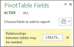
“Relationships between tables may be needed”
-
Step 1: Determine which tables to specify in the relationship
-
Step 2: Find columns that can be used to create a path from one table to the next
-
Notes about relationships
-
You’ll know whether a relationship exists when you drag fields from different tables onto the PivotTable Fields list. If you aren’t prompted to create a relationship, Excel already has the relationship information it needs to relate the data.
-
Creating relationships is similar to using VLOOKUPs: you need columns containing matching data so that Excel can cross-reference rows in one table with those of another table. In the time intelligence example, the Customer table would need to have date values that also exist in a time intelligence table.
-
In a data model, table relationships can be one-to-one (each passenger has one boarding pass) or one-to-many (each flight has many passengers), but not many-to-many. Many-to-many relationships result in circular dependency errors, such as “A circular dependency was detected.” This error will occur if you make a direct connection between two tables that are many-to-many, or indirect connections (a chain of table relationships that are one-to-many within each relationship, but many-to-many when viewed end to end. Read more about Relationships between tables in a Data Model.
-
The data types in the two columns must be compatible. See Data types in Excel Data Models for details.
-
Other ways to create relationships might be more intuitive, especially if you are not sure which columns to use. See Create a relationship in Diagram View in Power Pivot.
Example: Relating time intelligence data to airline flight data
You can learn about both table relationships and time intelligence using free data on the Microsoft Azure Marketplace. Some of these datasets are very large, requiring a fast internet connection to complete the data download in a reasonable period of time.
-
Start Power Pivot in Microsoft Excel add-in and open the Power Pivot window.
-
Click Get External Data > From Data Service > From Microsoft Azure Marketplace. The Microsoft Azure Marketplace home page opens in the Table Import Wizard.
-
Under Price, click Free.
-
Under Category, click Science & Statistics.
-
Find DateStream and click Subscribe.
-
Enter your Microsoft account and click Sign in. A preview of the data should appear in the window.
-
Scroll to the bottom and click Select Query.
-
Click Next.
-
Choose BasicCalendarUS and then click Finish to import the data. Over a fast internet connection, import should take about a minute. When finished, you should see a status report of 73,414 rows transferred. Click Close.
-
Click Get External Data > From Data Service > From Microsoft Azure Marketplace to import a second dataset.
-
Under Type, click Data.
-
Under Price, click Free.
-
Find US Air Carrier Flight Delays and click Select.
-
Scroll to the bottom and click Select Query.
-
Click Next.
-
Click Finish to import the data. Over a fast internet connection, this can take 15 minutes to import. When finished, you should see a status report of 2,427,284 rows transferred. Click Close. You should now have two tables in the data model. To relate them, we’ll need compatible columns in each table.
-
Notice that the DateKey in BasicCalendarUS is in the format 1/1/2012 12:00:00 AM. The On_Time_Performance table also has a datetime column, FlightDate, whose values are specified in the same format: 1/1/2012 12:00:00 AM. The two columns contain matching data, of the same data type, and at least one of the columns (DateKey) contains only unique values. In the next several steps, you’ll use these columns to relate the tables.
-
In the Power Pivot window, click PivotTable to create a PivotTable in a new or existing worksheet.
-
In the Field List, expand On_Time_Performance and click ArrDelayMinutes to add it to the Values area. In the PivotTable, you should see the total amount of time flights were delayed, as measured in minutes.
-
Expand BasicCalendarUS and click MonthInCalendar to add it to the Rows area.
-
Notice that the PivotTable now lists months, but the sum total of minutes is the same for every month. Repeating, identical values indicate a relationship is needed.
-
In the Field List, in “Relationships between tables may be needed”, click Create.
-
In Related Table, select On_Time_Performance and in Related Column (Primary) choose FlightDate.
-
In Table, select BasicCalendarUS and in Column (Foreign) choose DateKey. Click OK to create the relationship.
-
Notice that the sum of minutes delayed now varies for each month.
-
In BasicCalendarUS and drag YearKey to the Rows area, above MonthInCalendar.
You can now slice arrival delays by year and month, or other values in the calendar.
Tips: By default, months are listed in alphabetical order. Using the Power Pivot add-in, you can change the sort so that months appear in chronological order.
-
Make sure that the BasicCalendarUS table is open in the Power Pivot window.
-
On the Home table, click Sort by Column.
-
In Sort, choose MonthInCalendar
-
In By, choose MonthOfYear.
The PivotTable now sorts each month-year combination (October 2011, November 2011) by the month number within a year (10, 11). Changing the sort order is easy because the DateStream feed provides all of the necessary columns to make this scenario work. If you’re using a different time intelligence table, your step will be different.
“Relationships between tables may be needed”
As you add fields to a PivotTable, you’ll be informed if a table relationship is required to make sense of the fields you selected in the PivotTable.
Although Excel can tell you when a relationship is needed, it can’t tell you which tables and columns to use, or whether a table relationship is even possible. Try following these steps to get the answers you need.
Step 1: Determine which tables to specify in the relationship
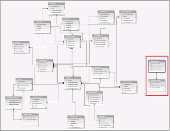
If your model contains just a few tables, it might be immediately obvious which ones you need to use. But for larger models, you could probably use some help. One approach is to use Diagram View in the Power Pivot add-in. Diagram View provides a visual representation of all the tables in the Data Model. Using Diagram View, you can quickly determine which tables are separate from the rest of the model.
Note: It’s possible to create ambiguous relationships that are invalid when used in a PivotTable or Power View report. Suppose all of your tables are related in some way to other tables in the model, but when you try to combine fields from different tables, you get the “Relationships between tables may be needed” message. The most likely cause is that you’ve run into a many-to-many relationship. If you follow the chain of table relationships that connect to the tables you want to use, you will probably discover that you have two or more one-to-many table relationships. There is no easy workaround that works for every situation, but you might try creating calculated columns to consolidate the columns you want to use into one table.
Step 2: Find columns that can be used to create a path from one table to the next
After you’ve identified which table is disconnected from the rest of the model, review its columns to determine whether another column, elsewhere in the model, contains matching values.
For example, suppose you have a model that contains product sales by territory, and that you subsequently import demographic data to find out if there is correlation between sales and demographic trends in each territory. Because the demographic data comes from a different data source, its tables are initially isolated from the rest of the model. To integrate the demographic data with the rest of your model, you’ll need to find a column in one of the demographic tables that corresponds to one you’re already using. For example if the demographic data is organized by region, and your sales data specifies which region the sale occurred, you could relate the two datasets by finding a common column, such as a State, Zip code, or Region, to provide the lookup.
Besides matching values, there are a few additional requirements for creating a relationship:
-
Data values in the lookup column must be unique. In other words, the column can’t contain duplicates. In a Data Model, nulls and empty strings are equivalent to a blank, which is a distinct data value. This means that you can’t have multiple nulls in the lookup column.
-
Data types of both the source column and lookup column must be compatible. For more information about data types, see Data types in Data Models.
To learn more about table relationships, see Relationships between tables in a Data Model.
Top of Page
Содержание
- Create one-to-one relationships
- Try it!
- What is a one-to-one relationship?
- Create one-to-one relationships overview
- Create a one-to-one relationship steps
- Relationships between tables in a Data Model
Create one-to-one relationships
Try it!
What is a one-to-one relationship?
One-to-one relationships are frequently used to indicate critical relationships so you can get the data you need to run your business.
A one-to-one relationship is a link between the information in two tables, where each record in each table only appears once. For example, there might be a one-to-one relationship between employees and the cars they drive. Each employee appears only once in the Employees table, and each car appears only once in the Company Cars table.
You might use one-to-one relationships if you have a table containing a list of items, but the specific information you want to capture about them varies by type. For example, you might have a contacts table in which some people are employees and other people are subcontractors. For the employees, you want to know their employee number, their extension, and other key information. For subcontractors, you want to know their company name, phone number, and bill rate, among other things. In this case, you’d create three separate tables—Contacts, Employees, and Subcontractors— and then create a one-to-one relationship between the Contacts and Employees tables and a one-to-one relationship between the Contacts and Subcontractors tables.
Create one-to-one relationships overview
You create one-to-one relationships by linking the index (usually the primary key) in one table and an index in another table which shares the same value. For example:

Often, the best way to create this relationship is to have the secondary table look up a value from the first table. For example, make the Car ID field in the Employees table a lookup field that looks for a value in the Car ID index from the Company Cars table. That way, you never accidentally add the ID of a car that doesn’t actually exist.
Important: When you create a one-to-one relationship, decide carefully whether to enforce referential data integrity for the relationship.
Referential data integrity helps Access to keep your data clean by deleting related records. For example, if you delete an employee from the Employees table, you also delete the benefits records for that employee from the Benefits table. But in some relationships, like this example, referential integrity doesn’t make sense: if we delete an employee, we don’t want the vehicle deleted from the Company Cars table, because the car will still belong to the company and will be assigned to someone else.
Create a one-to-one relationship steps
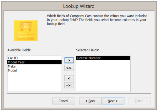
Create the one-to-one relationship by adding a lookup field to a table. (To learn how, see Build tables and set data types.) For example, to indicate which car has been assigned to a specific employee, you might add Car ID to the Employees table. Then, to create the relationship between the two fields, use the Lookup Wizard:
In Design View, add a new field, select the Data Type value, and then select Lookup Wizard.
In the wizard, the default is set to look up values from another table, so select Next.
Select the table that contains the key (usually a primary key) that you want to include in this table, and then select Next. In our example, you’d select the Company Cars table.
In the Selected Fields list, add the field that contains the key you want to use. Select Next.
Set a sort order and, if you prefer, change the width of the field.
On the final screen, clear the Enable Data Integrity check box and then select Finish.
Источник
Relationships between tables in a Data Model
Add more power to your data analysis by creating relationships amogn different tables. A relationship is a connection between two tables that contain data: one column in each table is the basis for the relationship. To see why relationships are useful, imagine that you track data for customer orders in your business. You could track all the data in a single table having a structure like this:
This approach can work, but it involves storing a lot of redundant data, such as the customer e-mail address for every order. Storage is cheap, but if the e-mail address changes you have to make sure you update every row for that customer. One solution to this problem is to split the data into multiple tables and define relationships between those tables. This is the approach used in relational databases like SQL Server. For example, a database that you import might represent order data by using three related tables:
Relationships exist within a Data Model—one that you explicitly create, or one that Excel automatically creates on your behalf when you simultaneously import multiple tables. You can also use the Power Pivot add-in to create or manage the model. See Create a Data Model in Excel for details.
If you use the Power Pivot add-in to import tables from the same database, Power Pivot can detect the relationships between the tables based on the columns that are in [brackets], and can reproduce these relationships in a Data Model that it builds behind the scenes. For more information, see Automatic Detection and Inference of Relationships in this article. If you import tables from multiple sources, you can manually create relationships as described in Create a relationship between two tables.
Relationships are based on columns in each table that contain the same data. For example, you could relate a Customers table with an Orders table if each contains a column that stores a Customer ID. In the example, the column names are the same, but this is not a requirement. One could be CustomerID and another CustomerNumber, as long as all of the rows in the Orders table contain an ID that is also stored in the Customers table.
In a relational database, there are several types of keys. A key is typically column with special properties. Understanding the purpose of each key can help you manage a multi-table Data Model that provides data to a PivotTable, PivotChart, or Power View report.
Though there are many types of keys, these are the most important for our purpose here:
Primary key: uniquely identifies a row in a table, such as CustomerID in the Customers table.
Alternate key (or candidate key): a column other than the primary key that is unique. For example, an Employees table might store an employee ID and a social security number, both of which are unique.
Foreign key: a column that refers to a unique column in another table, such as CustomerID in the Orders table, which refers to CustomerID in the Customers table.
In a Data Model, the primary key or alternate key is referred to as the related column. If a table has both a primary and alternate key, you can use either one as the basis of a table relationship. The foreign key is referred to as the source column or just column. In our example, a relationship would be defined between CustomerID in the Orders table (the column) and CustomerID in the Customers table (the lookup column). If you import data from a relational database, by default Excel chooses the foreign key from one table and the corresponding primary key from the other table. However, you can use any column that has unique values for the lookup column.
The relationship between a customer and an order is a one-to-many relationship. Every customer can have multiple orders, but an order can’t have multiple customers. Another important table relationship is one-to-one. In our example here, the CustomerDiscounts table, which defines a single discount rate for each customer, has a one-to-one relationship with the Customers table.
This table shows the relationships between the three tables ( Customers, CustomerDiscounts, and Orders):
Note: Many-to-many relationships are not supported in a Data Model. An example of a many-to-many relationship is a direct relationship between Products and Customers, in which a customer can buy many products and the same product can be bought by many customers.
After any relationship has been created, Excel must typically recalculate any formulas that use columns from tables in the newly created relationship. Processing can take some time, depending on the amount of data and the complexity of the relationships. For more details, see Recalculate Formulas.
A Data Model can have multiple relationships between two tables. To build accurate calculations, Excel needs a single path from one table to the next. Therefore, only one relationship between each pair of tables is active at a time. Though the others are inactive, you can specify an inactive relationship in formulas and queries.
In Diagram View, the active relationship is a solid line and the inactive ones are dashed lines. For example, in AdventureWorksDW2012, the table DimDate contains a column, DateKey, that is related to three different columns in the table FactInternetSales: OrderDate, DueDate, and ShipDate. If the active relationship is between DateKey and OrderDate, that is the default relationship in formulas unless you specify otherwise.
A relationship can be created when the following requirements are met:
Unique Identifier for Each Table
Each table must have a single column that uniquely identifies each row in that table. This column is often referred to as the primary key.
Unique Lookup Columns
The data values in the lookup column must be unique. In other words, the column can’t contain duplicates. In a Data Model, nulls and empty strings are equivalent to a blank, which is a distinct data value. This means that you can’t have multiple nulls in the lookup column.
Compatible Data Types
The data types in the source column and lookup column must be compatible. For more information about data types, see Data types supported in Data Models.
In a Data Model, you cannot create a table relationship if the key is a composite key. You’re also restricted to creating one-to-one and one-to-many relationships. Other relationship types are not supported.
Composite Keys and Lookup Columns
A composite key is composed of more than one column. Data Models can’t use composite keys: a table must always have exactly one column that uniquely identifies each row in the table. If you import tables that have an existing relationship based on a composite key, the Table Import Wizard in Power Pivot will ignore that relationship because it can’t be created in the model.
To create a relationship between two tables that have multiple columns defining the primary and foreign keys, first combine the values to create a single key column before creating the relationship. You can do this before you import the data, or by creating a calculated column in the Data Model using the Power Pivot add-in.
A Data Model cannot have many-to-many relationships. You can’t simply add junction tables in the model. However, you can use DAX functions to model many-to-many relationships.
Self-Joins and Loops
Self-joins are not permitted in a Data Model. A self-join is a recursive relationship between a table and itself. Self-joins are often used to define parent-child hierarchies. For example, you could join an Employees table to itself to produce a hierarchy that shows the management chain at a business.
Excel does not allow loops to be created among relationships in a workbook. In other words, the following set of relationships is prohibited.
Table 1, column a to Table 2, column f
Table 2, column f to Table 3, column n
Table 3, column n to Table 1, column a
If you try to create a relationship that would result in a loop being created, an error is generated.
One of the advantages to importing data using the Power Pivot add-in is that Power Pivot can sometimes detect relationships and create new relationships in the Data Model it creates in Excel.
When you import multiple tables, Power Pivot automatically detects any existing relationships among the tables. Also, when you create a PivotTable, Power Pivot analyzes the data in the tables. It detects possible relationships that have not been defined, and suggests appropriate columns to include in those relationships.
The detection algorithm uses statistical data about the values and metadata of columns to make inferences about the probability of relationships.
Data types in all related columns should be compatible. For automatic detection, only whole number and text data types are supported. For more information about data types, see Data types supported in Data Models.
For the relationship to be successfully detected, the number of unique keys in the lookup column must be greater than the values in the table on the many side. In other words, the key column on the many side of the relationship must not contain any values that are not in the key column of the lookup table. For example, suppose you have a table that lists products with their IDs (the lookup table) and a sales table that lists sales for each product (the many side of the relationship). If your sales records contain the ID of a product that does not have a corresponding ID in the Products table, the relationship can’t be automatically created, but you might be able to create it manually. To have Excel detect the relationship, you need to first update the Product lookup table with the IDs of the missing products.
Make sure the name of the key column on the many side is similar to the name of the key column in the lookup table. The names do not need to be exactly the same. For example, in a business setting, you often have variations on the names of columns that contain essentially the same data: Emp ID, EmployeeID, Employee ID, EMP_ID, and so on. The algorithm detects similar names and assigns a higher probability to those columns that have similar or exactly matching names. Therefore, to increase the probability of creating a relationship, you can try renaming the columns in the data that you import to something similar to columns in your existing tables. If Excel finds multiple possible relationships, then it does not create a relationship.
This information might help you understand why not all relationships are detected, or how changes in metadata—such as field name and the data types—could improve the results of automatic relationship detection. For more information, see Troubleshoot Relationships.
Automatic Detection for Named Sets
Relationships are not automatically detected between Named Sets and related fields in a PivotTable. You can create these relationships manually. If you want to use automatic relationship detection, remove each Named Set and add the individual fields from the Named Set directly to the PivotTable.
Inference of Relationships
In some cases, relationships between tables are automatically chained. For example, if you create a relationship between the first two sets of tables below, a relationship is inferred to exist between the other two tables, and a relationship is automatically established.
Products and Category — created manually
Category and SubCategory — created manually
Products and SubCategory — relationship is inferred
In order for relationships to be automatically chained, the relationships must go in one direction, as shown above. If the initial relationships were between, for example, Sales and Products, and Sales and Customers, a relationship is not inferred. This is because the relationship between Products and Customers is a many-to-many relationship.
Источник
Have you ever been in a VLOOKUP hell?
Its what happens when you have to write a lot of vlookup formulas before you can start analyzing your data. Every day, millions of analysts and managers enter VLOOKUP hell and suffer. They connect table 1 with table 2 so that all the data needed for making that pivot report is on one place. If you are one of those, then you are going to love Excel’s data model & relationships feature.

In simple words, this feature helps you connect one set of data with another set of data so that you can create combined pivot reports.
Practical Example – V(X)LOOKUP hell vs. Data Model heaven
Lets say you are looking sales data for your company. You have transaction data like below.
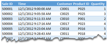
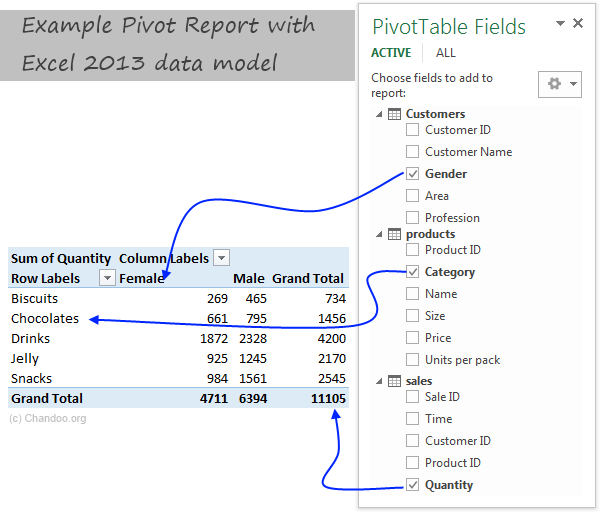
And you want to find out how many units you are selling by product category and customer’s gender.
Unfortunately, you only have product ID & customer ID.
With VLOOKUP Hell,
- You first fetch all the customer and product data and place them in separate ranges.
- Then write a vlookup formula to fetch product category, another to fetch customer gender.
- Then fill down the formulas for entire list of transactions.
- Now make a pivot table.
Assuming you have 30,000 transactions, you have to write 60,000 VLOOKUP formulas to create this one report!!!
With Data Model heaven,
- Create relationships between Sales, Products & Customer tables
- Create a pivot table
Creating a relationship in Excel – Step by Step tutorial
 First set up your data as tables. To create a table, select any cell in range and press CTRL+T. Specify a name for your table from design tab. Read introduction to Excel tables to understand more.
- Now, go to data ribbon & click on relationships button.
- Click New to create a new relationship.
- Select Source table & column name. Map it to target table & column name. It does not matter which order you use here. Excel is smart enough to adjust the relationship.

- Add more relationships as needed.
 First set up your data as tables. To create a table, select any cell in range and press CTRL+T. Specify a name for your table from design tab. Read introduction to Excel tables to understand more.
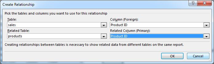
Using relationships in Pivot reports & analysis
- Select any table and insert a pivot table (Insert > Pivot table, more on Pivot tables).
- Make sure you check the “Add this data to data model” check box.

- In your pivot table field list, check “ALL” instead of “ACTIVE” to see all table names.
- Select fields from various tables to create a combined pivot report or pivot chart

Example: Category & Gender Sales Report
- Add category to row labels
- Add gender to column labels
- Add quantity to values
- and your report is ready!
Things to keep in mind when you using relationships
- Same data types in both columns: Columns that you are connecting in both tables should have same data type (ie both numbers or dates or text etc.)
- One to one or One to many relationships only: Excel 2013 supports only one to many or one to one relationships. That means one of the tables must have no duplicate values on the column you are linking to. (for example products table should not have duplicate product IDs).
- You can add slicers too: You can slice these pivot tables on any field you want (just like normal pivot tables). For example, you can further slice the above report on customer’s profession or product’s SKU size.
Benefits of Data Model based Pivot Tables
Once you have a data model in spreadsheet, you will enjoy several benefits (apart from multi-table pivots that is). They are,
- Distinct counts: This simple but often tricky to calculate number is easy to get once you have data model based pivot. Just go to value field settings and change the summary type to “Distinct count”. Here is a tip explaining how to get distinct counts in Excel pivots.
- Measures & DAX: Once you have a Data Model, you can unleash the full Power Pivot features on your workbook. You can create measures (using DAX language) and calculate things that are otherwise impossible with regular Excel. Here is an example of percentage of something calculation with DAX & Data Model, to get started.
- Pivots from data in other files & databases: You can combine data model with the abilities of Power Query to create pivots from data in other places. For example, you can make a pivot from sales data in SAP with customer data in CRM system. Here is an overview of what is Power Query?
- Pivots from more than 1mn rows of data: You can connect to very large datasets and make pivots from them with the help of data model. Here is a demo of how to set up data model for 1+mn rows of data.
- Convert Pivot Tables to formulas: Once you have a data model based pivot table, you can turn it in to a set of formulas. You can access this feature from “Analyze” ribbon. This will replace your pivot with a bunch of CUBE formulas. Here is an overview of CUBE formulas.
Drawbacks of Data Model:
Of course, its not all cup cakes and coffee with Data Model. There are a few drawbacks of data model based pivot tables.
- Compatibility: Data model & relationship feature is available only in Excel 2013 or above. This means, you cannot create or share such pivot reports with people using older versions of Excel.
- Not able to group data: In regular Pivot Tables, you can group numeric, data or text fields. But with data model pivot tables, you can no longer group data. You must create another table with the group mapping and use it as a relationship.
Download Example File
Click here to download Excel data model demo file. It contains 3 different tables and a combined pivot report (with slicer) to show you what is possible.
Do you use relationships?
Ever since discovering PowerPivot, I kind of stopped using VLOOKUP (or XLOOKUP) for most of my own analysis. Now that relationships are part of main Excel functionality, I am using them even more.
What about you? Are you using relationships & data model in Excel? What cool things are you doing with it? Share your tips with us using comments.
Want even more? Try PowerPivot
If you want even more out of your reports, then try PowerPivot. It is a new feature in Excel 2013 (available as add-in in Excel 2010) that can let you do lots of powerful analysis on massive amounts of data. Here is an introduction to PowerPivot.
Share this tip with your colleagues

Get FREE Excel + Power BI Tips
Simple, fun and useful emails, once per week.
Learn & be awesome.
-
41 Comments -
Ask a question or say something… -
Tagged under
data model, downloads, excel 2013, Learn Excel, pivot tables, relationship, vlookup
-
Category:
Excel Howtos, Pivot Tables & Charts

Welcome to Chandoo.org
Thank you so much for visiting. My aim is to make you awesome in Excel & Power BI. I do this by sharing videos, tips, examples and downloads on this website. There are more than 1,000 pages with all things Excel, Power BI, Dashboards & VBA here. Go ahead and spend few minutes to be AWESOME.
Read my story • FREE Excel tips book


Excel School made me great at work.
5/5

From simple to complex, there is a formula for every occasion. Check out the list now.

Calendars, invoices, trackers and much more. All free, fun and fantastic.

Power Query, Data model, DAX, Filters, Slicers, Conditional formats and beautiful charts. It’s all here.

Still on fence about Power BI? In this getting started guide, learn what is Power BI, how to get it and how to create your first report from scratch.
Related Tips
41 Responses to “How to use Excel Data Model & Relationships”
-
 Ashish Youngy says:
 Data is Excel 2013 behaves so much like a OLAP cube when using with PivotTables. And this is actually wow. Consider learning not just DAX but MDX too 🙂 Happy Excel
@Chandoo.. Have a nice and safe time in US. Best Wishes. And when they are publishing your interview in Entrepreneur 🙂
-
Buzz says:
I have been using PowerPivot in Excel 2010. My understanding was (via PowerPivot Pro blog) that Power Pivot would NOT be available in Excel 2013 in all versions; my recollection is that it was only going to be available in certain enterprise subscription editions. Thus, for individual users, it will no longer be available? For that reason I have moved some of my projects to Tableau, and do not expect to upgrade to Excel 2013.
Can you confirm the availability of Power Pivot for all Excel 2013 users , or will it be restricted and unavailable for some users?-
-
This is something that Excel is doing very poorly: letting people know what’s available with what. It also doesn’t help that they have so many packages and versions.
Excel Professional Plus has Power Pivot and Power View. I went through this last week. Spent 4 days upgrading from 365 Home Premium ($99 for the 1-yr subscription) to an additional $7/month for Professional Plus.
Also, one page on Microsoft’s site says that their Sharepoint Online Package 2 has Power View. NO! It’s not true. Sharepoint Online Package 2 will INTERACT with a spreadsheet that has PP or PV, Package 1 will not.
-
-
-
Just this weekend I upgraded from Home Premium to Professional Plus and spent time with Power View and PowerPivot.
Up to that point I never saw myself in VLOOKUP Hell, and it may not be going away any time soon. I’m surprised to discover how many of my clients are still on Excel 2003. And then I have Mac users who don’t have a lot of this great stuff available to them at all.
These are great features and I’m going to dive into the Data Models. Unfortunately, I suspect, for me, the practical use may be limited to blogposts because I can’t teach Power View in my workshops or send a client a spreadsheet that has a Power View in it.
-
thundom says:
Hi OZ,
I think the Microsoft would only upgrade the excel to a certain level instead of making it so powerful that it might threat their BI product. You know these «powerful» stuff can be easily done with a entry level crystal reports version.
Glad to listen to ur opinion on it.
I spent quite some time and energy on Excel and used it a lot, but now I am focusing energy on BI software like crystal reports.
-
thundom says:
We both know that based on the technology today. All the time we spend on the Macro and advanced function of Excel can be done easily with other softwares which costs only hundreds of bucks.
-
@Thondom
I don’t think Excel tries to be the solver of all problems
It is a generic tool
Which for about 95% of people will do what they want 95% of the time
There will always be specifics where specific custom software will do better than Excel
It is the commonness of Excel which means that I can send a model to you and it will work , most of the time, that is its strength, of course combined with its flexility in being able to be adapted to suit most needs-
thundom says:
Hi Hui,
You are right.But,
for the business and individual, who spend too much resource on Excel to meet their BI requirements and other processing requests.
Should they open their eyes to other ways to do it, in this age? Especially for many people try too much time to process stuff with thousands lines of macro programming.
It is just as when human being created gun fire, the martial arts would not be that effective.
Ppl need to be prodent when they choose their solution.
-
Hi guys, I just came across your conversation. I have an example of BI vs. Excel stuff. Here in Russia there is an ERP-system called «1C». It became a defacto standart for accounting, planning and BI / analytics. It is positioned as a flexible and powerful system and it really is.
But its reporting abilities aren’t user-friendly (or maybe just not me-friendly).
Many reports require programming and all those SQL things, so that is common for a company to have a couple of programmers who develop and code those reports.
So the common solution is to export data to Excel and then process it to be more suitable for further analysis or reporting.
Well, it’s obviously not a rule of thumb that special BI software can outperform Excel in day-to-day routine.
-
-
-
-
-
Tris says:
Hi Chandoo, thanks for publishing great Excel information. Pardon the ignorance as I havent used Data Model nor PowerPivot. But having seen your video clip on PowerPivot, how does Data Model differ from PowerPivot — the «process» seems familiar? Have a great day! And Excel to new heights! Regards,
-
@Tris, one main difference is that Data Model is part of Excel Home Premium. You’ve got to upgrade to ProPlus to get PowerPivot and Power View.
-
-
Nolberto says:
Excellent posting, some pride themselves for having sheets with thousands of formulas or complicated formulas, but in the end the important thing is to work as little as possible.
-
@Nolberto let’s not gloat yet. Some people are forced to have thousands of complicated formulas when they don’t have the fancy tools. I’m sad for the 2003 users who have to use SUMPRODUCT when the rest of us have SUMIFS available.
In the end, I think the important thing is clean, trustworthy data—however you arrive at it. People survived more than 300 years with slide rules and paper. No PowerPivot for the Wright Brothers.
-
-
koi says:
hi chandoo,
i added 2 column into sales, 1st column vlookup customer ID to CUST sheet to get the male or female, then 2nd column vlookup Product ID to Product sheet to get the product name, then after that i make pivot table out of sales sheet.
but then the result is really different from yours
the purposes is just try to do the vlookup vs add to data model to see if they get same result
thanks
-
Hi Koi,
We are using gender vs. category in the report. Can you try with that? I am sure the results will match.
-
-
koi says:
ups sorry, didnt see that you’re filtering using slicer..then it is good now the result are same with less effort 🙂
thanks
-
SPrasad says:
Hi Chandoo, .I am interested to know whether we can build a star schema or snow flake data models through relations in Excel? (trying to correlate with Qlikview)
-
Hi there,
You can create a Star schema for sure. Snow-flake is possible too. As long as all relationships are one to many (or one to one) anything is possible.
-
Nestavaro says:
What if customer.profession change its value after sometime?
Supposed we have monthly data for Sales. What if one customer is a doctor in Feb, then a pilot in October, for example?How to build data model for such that situation?
Thank you.
-
-
-
[…] Introduction to Excel 2013 Data Model & Relationships […]
-
Raghavendra Shanbog says:
Hello ,
I find this option similar to that of MS Access.
In MS Access as well we have relationship concept and once you create a relationship, you can start creating number of queries based on that.
But MS Access is not so user friendly and basically its database. Good that we are getting those options/functions in Excel.
Thanks for sharing this info.Regards,
Raghavendra Shanbog -
What is star schema and snow flake.??? Can we have next article on that if it is useful for us???
-
Roberto says:
Hi there, can anyone help? I tried testing this out in Excel using two tables. When I go to the Data tab the Relationships button does not appear at all. I am using Microsoft version 14.0.4760.1000, Microsoft Office Professional Plus 2010. Does this version have this capability? Or is there an add-in required?
-
[…] even a layperson can perform if they have the almighty Excel 2010 and PowerPivot installed. Or Excel 2013′s Data Model, which lets you mash up data from Excel Tables and serve them up directly as PivotTables with not a […]
-
Chandeep Chhabra says:
Chandoo/Hui,
The dates grouping feature does not seem to work in Data Model. Is that true or am I making a mistake somewhere?
-
Jay says:
I don’t think this is really for «lookups»…
Try creating a pivot with sale ID and customer name in row fields. It will give you ALL customer names per sale ID.
You’d need to use RELATED function in a new column in powerpivot if you want something equivalent to «vlookup»
-
Aslam says:
Please explain the difference between data model and power pivot, the functions of both of them are different and similar
thanks -
[…] Handling large volumes of data in Excel—Since Excel 2013, the “Data Model” feature in Excel has provided support for larger volumes of data than the 1M row limit per worksheet. Data Model also embraces the Tables, Columns, Relationships representation as first-class objects, as well as delivering pre-built commonly used business scenarios like year-over-year growth or working with organizational hierarchies. For several customers, the headroom Data Model is sufficient for dealing with their own large data volumes. In addition to the product documentation, several of our MVPs have provided great content on Power Pivot and the Data Model. Here are a couple of articles from Rob Collie and Chandoo. […]
-
Bernadette Savage says:
I need to use a slicer to allow a user to select vendor by name. In the background, I need to obtain the vendor ID to link to multiple datasets where the name may not be spelled consistently. Any advice?
-
Andrea says:
I’ve tried this in Excel 2016. It works great.
I can even create Cube Formulas on the Data model after I’ve inserted the pivot table.
Just for the fun of it, I tried to see if I could do Cube Formulas without creating the pivot table in advance. I can define Cube members, but it seems as if the measure part is playing tricks on me.I can’t get a Cube Value for Chocolates sold to Male customers.
With the Pivot created the formula looks like this (and works fine)
=CUBEVALUE(«ThisWorkbookDataModel»;»[Customer].[Gender].&[Male]»;»[Product].[Category].&[Chocolates]»;»[Measures].[Sum of Quantity]»)Does anyone know how I can solve this, or am I asking the impossible?
-
Kwabena Anaafi says:
I want to see the video on this topic
-
nestavaro says:
What if customer.profession change its value after sometime?
Supposed we have monthly data for Sales. What if one customer is a doctor in Feb, then a pilot in October, for example?How to build data model for such that situation?
Thank you.
-
In such case, you need to make relationships based on two columns. This kind of feature is not supported in Excel. You can use Power Query to merge tables based on multiple columns and return a consolidated giant table to Excel for reporting.
-
-
nestavaro says:
Is it able in MS Access?
I have never used access before. -
faisal says:
thanks chandooo your article is very helpfull for troubling peoples’ especially in office environment under boss pressure.
-
Ron says:
Here is an introduction to PowerPivot.
The link above is broken
-
Venkatesh says:
Hi. This has really taken my interest.. I have huge data tables to work with…and I use vlookup to fetch certain data. I have different data in different sheets…
Like customer sales (customer code, product code,qty, piece rate, total amount, branch code) data in one sheet
Branch details in another (branch code, branch address, state , region)
Customer Geographical Data in third sheet (region, region name)
Product details in fourth sheet (product code, product description and related)Now I use a vlookup to get branch name, state and product name respectively into my main sheet.
Now what I want is
customer code, product code,qty, piece rate, total amount, branch code) data in one sheet, branch address, state , region, region name, product description
Can’t his be done thru data model… I tried but it’s not working… Eitherway, I will gonthru thr session on e again and give a try… Any help, is appreciated. Thankyou
-
Achyutanand Khuntia says:
Dear All,
i am striving to do reverse relationship in Power pivot ,
example : —
1 — Data sheet
2. — Source datastep to stops — import first data sheet in power piovt and then source data , made relationship with both sheet , after created relationship i am able to do put related formula in source data sheet only (=releted(‘Source data'[Amount]), if i go to put formula in data sheet , parameter of Source data are not visible ,
could someone educate me how can i do , and utilize related formula in data sheet.
Leave a Reply
Excel is not a database for sure; however, people tend to use it as a database. Since primary versions of Excel, people keep on using it for making the connection between different tables with the help of VLOOKUP, INDEX, MATCH, SUMIF, etc.
Making reports was never an easier task as handling larger datasets is a tricky thing. Excel Data Model is a true blessing that lets you save time using automatic data reports. Here we will talk about how to create a relationship in Excel. Using the Data Model, you can make the connection between two tables and a figure of the relationship in a pivot table side by side.
To understand how to create a relationship between two tables in Excel, let’s start with a quick overview of the relationship.
What is a Relationship?
Merging two different tables result in a relationship:
- Within two tables, you must find a mutual column. However, you don’t need to allocate the same name to the columns.
- The new column must have distinctive entries only.
Hundreds of tables exist in relational databases that make such kinds of relationships. In Excel, you can make a fundamental relational structure using the Data Model option. Suppose an Order data table and a Sales data table, both contain a mutual column State. And both tables have duplicate data in these columns, so you are not allowed to add that column to the new table. You have to skip the State column.
Why Is It Important to Make a Relationship?
Realizing the importance of anything helps you understand why you should use it. Just a single data table is not enough to provide all the information needed to make a report. It often happens in many cases, that’s why the need of creating relationship tables in Excel comes up.
Taking the above example, making a report about a person who marked the order is not likely to be placed in the Sales data table. Making a relationship between two tables Order and Sales just need the Order ID to extract the name from the table to be used in the Sales report.
Note: Remember that PivotTables replace the term “column” with “field.”
The Fundamental Needs
Before understanding how to create a relationship in Excel, let’s understand the basics of this process. For this, you must have Power Pivot and Power Query to complete the process of making an Excel Data Model.
Below you will find out the starting procedure:
How to Get Power Pivot
For Excel 2010, the Power Pivot add-in is needed to be downloaded from Microsoft. Once the downloading is complete, make sure to install it properly on your system.
For Excel 2013, you don’t need to download or install anything manually as the Office Pro Plus edition of Excel 2013 has a built-in Power Pivot. You just need to activate it before using it.
To activate the Power Pivot follow the steps given below:
- Open the Excel workbook and click the Ribbon on the File.
- Click on the Options and you will see a window of Excel Options.
- Next, click on Add-ins.
- On the Manage box, click the drop-down menu and choose COM Add-ins.
- Press Go and choose the checkbox for Microsoft Power Pivot for Excel.
How to Get Power Query (Get & Transform)
- For Excel 2010, similar to the Power Pivot add-in, you need to download the Power Query add-in from Microsoft.
- Once the downloading is complete, you need to install it properly and you will start seeing the Power Query on the Ribbon.
- For Excel 2013, again you don’t need to download and install anything as there is a built-in Power Query. You just have to activate it by following the same steps you did to make Power Pivot functional in Excel 2013.
- For Excel 2016 and Later, you have to go to the Data tab on Excel Ribbon to get the Power Query (Get & Transform).
How to Create a Relationship in Excel – Step-by-Step Guide
- At first, you need to set your data as tables. In the process of making a table, you have to select a random cell in the range and press Ctrl + T. From the design tab, you have to spell out a name for the table.
- Next, you have to open the data ribbon & click on the relationships button.
- To make a new relationship, you have to click on the New.
- Choose Source table & column name. To mark the table and column name, you need to record it. It does not matter what order you are using for making this relationship table. You should never underestimate the power of Excel no matter what.

- Now, you can add more relationships as required.
Things to Consider About Relationship
Keep in mind that VLOOKUPS and making relationships both are alike somehow. Duplicate data columns are needed for Excel to cross-reference rows of one table to the other.
While using relationships, you must keep in mind that there must be similar data types in both columns. For instance, connecting columns of both tables must have the same data type.
Excel 2013 holds up one to one or one to many relationships only. It simply shows that one of the tables is free from duplicate values on the linking columns. For instance, the products table must not contain similar product IDs.
Slicing these Pivot Tables is easier just the way you can do with normal Pivot Tables. For instance, you can further slice the products report on the products prices.
Do You Like Using Relationships?
Well, the relationships feature has replaced many tools and things. People skipped VLOOKUP for most of their analysis. Now, relationships features have become the central part of Excel, which is being used more and more.
You should try using relationship tables and data models in Excel. Elaborate your thoughts about using relationship tables and data models with us. I hope that you got an idea about how to create a relationship in Excel. Now, try it, share it and practice it.
I have a workbook for controlling attendance of students on a course, modelled on many worksheets.
The first worksheet have the cadastral data for all students. The other ones have attedence data of each month.
I need to dinamically update the first column of the attendance worksheets according with students column on cadastral data worksheet.
VLOOKUP or MATCH/INDEX seems not to be a good solution because data can be added on cadastral data worksheet, and I need to always re-organize students to alphabetical order.
For example:
Cadastral Data:
Student | (many data ccolumns)
Ann | data
Charlie | data
Jack | data
February Attendence:
Student | Day 01 | Day 02 | Day 03 …
Ann | ok ok nok
Charlie | ok ok ok
Jack | ok nok ok
If I use VLOOKUP or INDEX/MATCH and add Daniel on cadastral data and then sort alphabetically, I’ll have this issue:
Cadastral Data:
Student | (many data ccolumns)
Ann | data
Charlie | data
Daniel | data
Jack | data
February Attendence:
Student | Day 01 | Day 02 | Day 03 …
Ann | ok ok nok
Charlie | ok ok ok
Daniel | ok nok ok
Jack |
Jack Data changed to Daniel.
Is there a simple solution for this?