One row to multiple rows in excel

In Excel — split a row into multiple rows

I would like an Excel formula that will help me split entries in a single row to be split into multiple rows as shown in the second table in the image. Would appreciate any help:

Page 2

Attempted the formulas shared in How do I split one row into multiple rows with Excel? however it doesn’t work if Name column entries are duplicated.

2 Answers 2

To transform your Table1 to Table2 , as in your first screen shot, you can use Power Query available in Excel 2010+ either as a free add-in from MS, or built-in in later versions.

Although the transformation can be done from the GUI, that will return errors if you expand the number of columns in your data. So you need to modify the actual M-Code that is generated.

• I have assumed that columns, if added, will always be in Groups of 4 ( Task Name | Start Time | End Time | Consumed Time ).
• I have Also assumed that the Consumed Time column contains formatted Integers. If it really contains text, some changes will be required in the Query.

• Import the Table ( PQ will turn a range into a Table, or you can do this yourself)
• Select Project Name and unpivot other columns
• Because this has been converted into a Table, the duplicate column names in the original range will be converted by have a sequential number appended.
  • To remove that number after the unpivot, select the new Attribute column
    • Split the column on the transition from letter to digit
    • Delete the column with the numbers.
• For grouping of the data into appropriate rows:
  • Add Index column (base zero)
  • Based on the Index column, add an Integer/Divide column dividing by 4
  • Delete the Index column
• Now we Group By the Integer-Division and Project Name columns with Operation:= All Rows (no aggregation)
• We add a Custom Column which converts the resultant table into a List and then
• Extract the values from the List using a semicolon separator (or some other token not likely to appear in the data).
• We then Split those values into separate Columns using the semicolon as the delimiter
• Remove the extraneous columns
• Rename the columns so as to be the same names as the first five names in the original table.
• Change the data type of the table columns to Text, Time and Whole number as warranted
• Sort the rows by Project Name and Task Name
• Load back to the worksheet.

This query can be refreshed if you change anything, or add rows or column groups.

If you just paste the code into the Advanced Editor of a blank query, you will need to change Table3 in line 2 to whatever the name of your table is on your worksheet.

Источник

How do I split one row into multiple rows with Excel?

I have a product database in Excel with several hundred entries, each of which has from 1 to 3 «tiers» of pricing: Standard, Deluxe, and Premium. Each tier has its own SKU (A, B, or C added on to the end of the base SKU) and price. My data is like this:

How would I go about getting the data to look like this:

If it helps, I’m going to be importing these products into a Magento installation.

Thank you in advanced.

2 Answers 2

Those tasks are usually faster with VBA. In fact, it took me

10 minutes to set it up.
I’m assuming your data is in column A to column H.

Go to Excel » Developer » Visual Basic » On the left pane open sheet1 (or) the sheet where your data resides » Insert the code at the right window » Run the code

VBA code

Explanation

It was my intention to keep the code as short as possible to explain it better. Basically we use two loops. The outer loop ( i ) is for the rows and the inner loop ( j ) for the price columns.

We heavily use cells(rowNumber,columnNumber) to read/write cells.

Line 2| Start a loop from row 2 to your last row. We iterate through every used row

Line 3| Start a second loop from 0 to 2 (that are actually 3 loops, one for every Price column)

Line 4| We use this inner loop to check for values in our current row and column Price A, then Price B and in the last loop Price C. If we find a value in a Price column, we go on and copy cells. If no Price is inserted, we do nothing and go on to the next Price column

Line 5| Count up a counter to know how many rows we already copied,
so we know after what row we can copy our current row

Line 6| Copy the name column

Line 7| Copy the description column

Line 8| Copy the Price A or B or C column depending on what inner loop we currently are

Line 9| Copy the SKU A or B or C column depending on what inner loop we currently are

Result screenshot

Here is a worksheet function solution. The formulas are a bit dense, so be warned, but this will give what you want.

1. In the first row of your new table, under Name , enter a direct reference to the first Name in your data. In your example, you would enter =A2 where A2 is the first name listed in your data. In the example screenshot I’ve provided below, this formula goes in A8 . All following formulas will follow the layout used in the screenshot. You will of course have to update all range references to match your sheet(s).
2. In the cell below this, enter the following formula: This basically checks how many rows there should be for the name listed above (in A9 ), and if the number of rows already in your new table matches this, then it moves on to the next name. If not, another row for the name above will be added.
   Fill this formula down as far as you need to (until it returns a 0 instead of a name).
3. In the first row under Description enter the following formula and fill down.
4. In the first row under SKU , paste the following formula into the formula bar and press Ctrl + Shift + Enter . This is an array formula; if entered correctly the formula will appear in the formula bar enclosed in curly brackets. Fill this formula down your table (each instance should likewise appear in curly brackets).
5. Similarly, in the first row under Price , paste the following formula into the formula bar and enter it as an array formula (by pressing Ctrl + Shift + Enter ). Fill down, and this should complete your table.

Источник

Turn one row into multiple rows in Excel

I have multiple items that are available in multiple distribution centers (i.e., a many-to-many relationship). There is currently one row per item, with one column for each distribution center. A cell in the row for item X and the column for distribution center Y is marked with the code for distribution center Y if item X is available there and blank otherwise. An item with multiple distribution centers will have multiple distribution center codes (in their respective columns). So the current sheet looks like:

Columns C through R contain other attributes of the items, such as UPC code, cost, and price, which are not relevant to this question. My actual sheet has 18 distribution centers, spanning columns S through AJ ; I reduced that to get the example to fit into Stack Exchange’s window.

I need to have a single distribution center column, with a single distribution code per row, and then duplicate the rows as needed for items that currently contain multiple codes. The result should look like:

where cells A3:R3 , A4:R4 , and A5:R5 , contain the same information.

The only way I can think of doing this, which would be time consuming, would be to copy the item number into multiple rows; and in the column that has the distribution code I would change code for the item that is available in each distribution center. I will be doing this for 900 items. Is there an easier way to do this?

Источник

Microsoft Excel: Splitting One Cell Row into Multiple Rows

With Excel, you can split one cell into multiple rows or a comma delimited cell into multiple rows. This tutorial explains how.

If your job requires you to manipulate or organize large amounts of data, you probably spend lots of time working with Microsoft Excel for a variety of purposes. Excel is the gold-standard spreadsheet for manipulating data data and generating graphs.

You also need to deal with formatting and splitting data within Excel using formulas and filters.

Video Tutorial

Step-by-step directions

The process of converting one delimited row into multiple rows is divided into two stages.

1. Convert a delimited row string into multiple columns.
2. Transpose multiple columns into multiple rows.

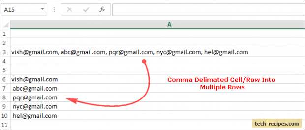
Let us assume that you have the following data in a cell as one row, which is separated by a comma (,). This means the comma is a delimiter in this string.

vish@gmail.com, abc@gmail.com, pqr@gmail.com, nyc@gmail.com, hel@gmail.com

Stage 1 – Convert a Delimited Row String into Multiple Columns

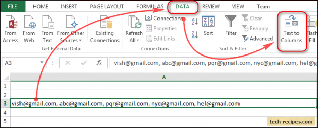
1. Select the delimited row that you want to convert into multiple rows.
2. From the top ribbon on the Data tab in the Data tool group, click Text to Columns.

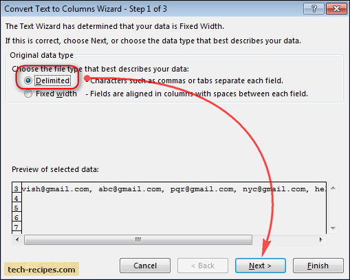
3. In Step 1 of the Convert Text to Columns Wizard, select Delimited, and then click Next.

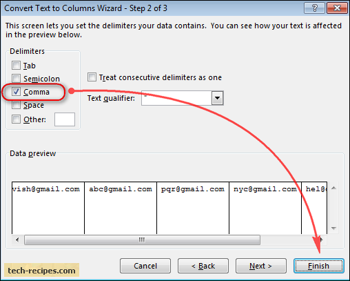
4. In Step 2, select the Comma checkbox, and clear all other checkboxes. In the Data preview, you can see the email addresses separated into multiple columns. Then click Finish.

Now, you can see the delimited row is separated into six different columns from A to F. We have completed the first stage, converting a delimited string into multiple columns. Now, we will complete Stage 2: Transpose.

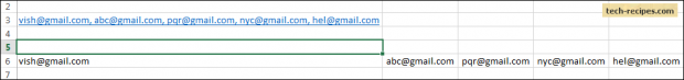
Stage 2 – Transpose Multiple Columns into Multiple Rows

1. Select the range of columns, in this case columns A to F.
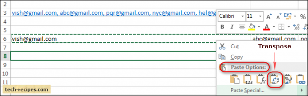
2. Press CTRL + C, or click Copy on the Home tab.
3. Select the cell where you want your first row to be. Right on that cell, from Paste Options, select the fourth option which is Transpose.

The video tutorial will take you through the same steps.

Источник

How to Insert Multiple Rows in Excel

In the last few decades, Microsoft has grown by leaps and bounds and so are its fabulous products. Microsoft Excel is one such product that has grown immensely. It has wonderful features and options to make your tasks easier. But one feature that it lacks is the ability to insert multiple rows. The default insert option that Excel has allows you to insert only one row at a time.

This can be very annoying in cases where you have to insert multiple rows in your spreadsheet. And this is what I am going to write today. In this post, I will present a few ways which allow you to insert multiple rows.

Table of Contents

Method 1 – By making use of the repeat functionality of excel:

This is the simplest way to insert multiple rows in your excel spreadsheet. In this method, we will first add one row manually to the excel sheet then repeat that action multiple times. Follow the below steps to use this method:

• Open your spreadsheet, and first of all insert one row to your excel sheet manually.
• Then simply repeatedly press the “F4” key on your keyboard, till the required number of rows are inserted.
• This will repeat your last action and the rows will be added.

Method 2 – By using the insert functionality:

In this method, we will use a hidden feature that excel offers to insert multiple rows to your sheet. Follow the below steps to use this method:

• Open your spreadsheet and select the number of rows that you want to insert to your sheet. It doesn’t matter if the rows are empty but they must include the place where you want to perform the insert.

• Now simply right-click anywhere in the previously selected range and select the ‘Insert’ option.
• Now excel will ask you whether to shift the cells down or shift them to right. Select the option ‘Shift Cells Down’ and multiple cells will be inserted in the location.

Method 3 – By using the insert copied cells functionality:

In this method, we are going to take the advantage of the “Insert Copied Cells” functionality that excel has. Follow the below steps to use this method:

• First of all select multiple rows in your spreadsheet, by multiple I mean they should be equal to the number of rows that you want to insert.
• Next, copy these rows and scroll to the place where you want to insert multiple rows.

• Right-click and select the option ‘Insert Copied Cells’ and this will insert multiple rows at that place.

Method 4 – Programmatically inserting multiple rows in excel:

Although this method is a bit complex than the first three, still this can be used if you are more inclined towards the coding side. Follow the below steps to use this method:

• Navigate to the ‘View’ tab on the top ribbon, click on the ‘Macros’ button.
• Now type the name for the macro say “Insert_Lines” (without quotes) and hit the create button.
• Next, a VBA editor will be opened, simply paste the below macro code after the first line.

• Now comes the important thing, in the above macro the range is (“A20:A69”). The first parameter i.e. A20 tells the position from where you wish to insert the rows and the second parameter .i.e. A69 is the number of rows to be inserted added with the start position and subtracted by 1 (for instance: If you want to insert 50 rows starting from A20 then the second parameter of the range should be (50+20-1), so the range will be (“A20:A69”))
• After adding the code you can press the “F5” key and the code will insert the required rows.
• This macro is referenced from the Microsoft article: http://support.microsoft.com/kb/291305

So, these were the few methods to insert multiple rows in excel. If you know some other ways then feel free to comment below.

Subscribe and be a part of our 15,000+ member family!

Now subscribe to Excel Trick and get a free copy of our ebook «200+ Excel Shortcuts» (printable format) to catapult your productivity.

Источник