Office microsoft excel formulas - Word и Excel - помощь в работе с программами

Overview of formulas in Excel

Get started on how to create formulas and use built-in functions to perform calculations and solve problems.

Important: The calculated results of formulas and some Excel worksheet functions may differ slightly between a Windows PC using x86 or x86-64 architecture and a Windows RT PC using ARM architecture. Learn more about the differences.

Important: In this article we discuss XLOOKUP and VLOOKUP, which are similar. Try using the new XLOOKUP function, an improved version of VLOOKUP that works in any direction and returns exact matches by default, making it easier and more convenient to use than its predecessor.

Create a formula that refers to values in other cells

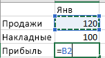
Select a cell.
Type the equal sign =.

Note: Formulas in Excel always begin with the equal sign.
Select a cell or type its address in the selected cell.
Enter an operator. For example, – for subtraction.
Select the next cell, or type its address in the selected cell.
Press Enter. The result of the calculation appears in the cell with the formula.

See a formula

When a formula is entered into a cell, it also appears in the Formula bar.
To see a formula, select a cell, and it will appear in the formula bar.

Enter a formula that contains a built-in function

Select an empty cell.
Type an equal sign = and then type a function. For example, =SUM for getting the total sales.
Type an opening parenthesis (.
Select the range of cells, and then type a closing parenthesis).
Press Enter to get the result.

Download our Formulas tutorial workbook

We’ve put together a Get started with Formulas workbook that you can download. If you’re new to Excel, or even if you have some experience with it, you can walk through Excel’s most common formulas in this tour. With real-world examples and helpful visuals, you’ll be able to Sum, Count, Average, and Vlookup like a pro.

Formulas in-depth

You can browse through the individual sections below to learn more about specific formula elements.

A formula can also contain any or all of the following: functions, references, operators, and constants.

Parts of a formula

1. Functions: The PI() function returns the value of pi: 3.142…

2. References: A2 returns the value in cell A2.

3. Constants: Numbers or text values entered directly into a formula, such as 2.

4. Operators: The ^ (caret) operator raises a number to a power, and the * (asterisk) operator multiplies numbers.

A constant is a value that is not calculated; it always stays the same. For example, the date 10/9/2008, the number 210, and the text «Quarterly Earnings» are all constants. An expression or a value resulting from an expression is not a constant. If you use constants in a formula instead of references to cells (for example, =30+70+110), the result changes only if you modify the formula. In general, it’s best to place constants in individual cells where they can be easily changed if needed, then reference those cells in formulas.

A reference identifies a cell or a range of cells on a worksheet, and tells Excel where to look for the values or data you want to use in a formula. You can use references to use data contained in different parts of a worksheet in one formula or use the value from one cell in several formulas. You can also refer to cells on other sheets in the same workbook, and to other workbooks. References to cells in other workbooks are called links or external references.

The A1 reference style

By default, Excel uses the A1 reference style, which refers to columns with letters (A through XFD, for a total of 16,384 columns) and refers to rows with numbers (1 through 1,048,576). These letters and numbers are called row and column headings. To refer to a cell, enter the column letter followed by the row number. For example, B2 refers to the cell at the intersection of column B and row 2.

To refer to	Use
The cell in column A and row 10	A10
The range of cells in column A and rows 10 through 20	A10:A20
The range of cells in row 15 and columns B through E	B15:E15
All cells in row 5	5:5
All cells in rows 5 through 10	5:10
All cells in column H	H:H
All cells in columns H through J	H:J
The range of cells in columns A through E and rows 10 through 20	A10:E20

Making a reference to a cell or a range of cells on another worksheet in the same workbook

In the following example, the AVERAGE function calculates the average value for the range B1:B10 on the worksheet named Marketing in the same workbook.

1. Refers to the worksheet named Marketing

2. Refers to the range of cells from B1 to B10

3. The exclamation point (!) Separates the worksheet reference from the cell range reference

Note: If the referenced worksheet has spaces or numbers in it, then you need to add apostrophes (‘) before and after the worksheet name, like =’123′!A1 or =’January Revenue’!A1.
The difference between absolute, relative and mixed references
1. Relative references A relative cell reference in a formula, such as A1, is based on the relative position of the cell that contains the formula and the cell the reference refers to. If the position of the cell that contains the formula changes, the reference is changed. If you copy or fill the formula across rows or down columns, the reference automatically adjusts. By default, new formulas use relative references. For example, if you copy or fill a relative reference in cell B2 to cell B3, it automatically adjusts from =A1 to =A2.
  
  Copied formula with relative reference
2. Absolute references An absolute cell reference in a formula, such as $A$1, always refer to a cell in a specific location. If the position of the cell that contains the formula changes, the absolute reference remains the same. If you copy or fill the formula across rows or down columns, the absolute reference does not adjust. By default, new formulas use relative references, so you may need to switch them to absolute references. For example, if you copy or fill an absolute reference in cell B2 to cell B3, it stays the same in both cells: =$A$1.
  
  Copied formula with absolute reference
3. Mixed references A mixed reference has either an absolute column and relative row, or absolute row and relative column. An absolute column reference takes the form $A1, $B1, and so on. An absolute row reference takes the form A$1, B$1, and so on. If the position of the cell that contains the formula changes, the relative reference is changed, and the absolute reference does not change. If you copy or fill the formula across rows or down columns, the relative reference automatically adjusts, and the absolute reference does not adjust. For example, if you copy or fill a mixed reference from cell A2 to B3, it adjusts from =A$1 to =B$1.
  
  Copied formula with mixed reference
The 3-D reference style

Conveniently referencing multiple worksheets If you want to analyze data in the same cell or range of cells on multiple worksheets within a workbook, use a 3-D reference. A 3-D reference includes the cell or range reference, preceded by a range of worksheet names. Excel uses any worksheets stored between the starting and ending names of the reference. For example, =SUM(Sheet2:Sheet13!B5) adds all the values contained in cell B5 on all the worksheets between and including Sheet 2 and Sheet 13.
- You can use 3-D references to refer to cells on other sheets, to define names, and to create formulas by using the following functions: SUM, AVERAGE, AVERAGEA, COUNT, COUNTA, MAX, MAXA, MIN, MINA, PRODUCT, STDEV.P, STDEV.S, STDEVA, STDEVPA, VAR.P, VAR.S, VARA, and VARPA.
- 3-D references cannot be used in array formulas.
- 3-D references cannot be used with the intersection operator (a single space) or in formulas that use implicit intersection.
What occurs when you move, copy, insert, or delete worksheets The following examples explain what happens when you move, copy, insert, or delete worksheets that are included in a 3-D reference. The examples use the formula =SUM(Sheet2:Sheet6!A2:A5) to add cells A2 through A5 on worksheets 2 through 6.
- Insert or copy If you insert or copy sheets between Sheet2 and Sheet6 (the endpoints in this example), Excel includes all values in cells A2 through A5 from the added sheets in the calculations.
- Delete If you delete sheets between Sheet2 and Sheet6, Excel removes their values from the calculation.
- Move If you move sheets from between Sheet2 and Sheet6 to a location outside the referenced sheet range, Excel removes their values from the calculation.
- Move an endpoint If you move Sheet2 or Sheet6 to another location in the same workbook, Excel adjusts the calculation to accommodate the new range of sheets between them.
- Delete an endpoint If you delete Sheet2 or Sheet6, Excel adjusts the calculation to accommodate the range of sheets between them.

The R1C1 reference style

You can also use a reference style where both the rows and the columns on the worksheet are numbered. The R1C1 reference style is useful for computing row and column positions in macros. In the R1C1 style, Excel indicates the location of a cell with an «R» followed by a row number and a «C» followed by a column number.

Reference	Meaning
R[-2]C	A relative reference to the cell two rows up and in the same column
R[2]C[2]	A relative reference to the cell two rows down and two columns to the right
R2C2	An absolute reference to the cell in the second row and in the second column
R[-1]	A relative reference to the entire row above the active cell
R	An absolute reference to the current row

When you record a macro, Excel records some commands by using the R1C1 reference style. For example, if you record a command, such as clicking the AutoSum button to insert a formula that adds a range of cells, Excel records the formula by using R1C1 style, not A1 style, references.

You can turn the R1C1 reference style on or off by setting or clearing the R1C1 reference style check box under the Working with formulas section in the Formulas category of the Options dialog box. To display this dialog box, click the File tab.

Top of Page

Need more help?

You can always ask an expert in the Excel Tech Community or get support in the Answers community.

Полные сведения о формулах в Excel

Начните создавать формулы и использовать встроенные функции, чтобы выполнять расчеты и решать задачи.

Важно: Вычисляемые результаты формул и некоторые функции листа Excel могут несколько отличаться на компьютерах под управлением Windows с архитектурой x86 или x86-64 и компьютерах под управлением Windows RT с архитектурой ARM. Подробнее об этих различиях.

Важно: В этой статье мы обсудим похожие проблемы с просмотром и просмотром. Попробуйте использовать новую функцию ПРОСМОТРX , улучшенную версию функции ВЛОП, которая работает в любом направлении и по умолчанию возвращает точные совпадения, что упрощает и удобнее в использовании, чем предшественницу.

Создание формулы, ссылающейся на значения в других ячейках

Выделите ячейку.
Введите знак равенства «=».

Примечание: Формулы в Excel начинаются со знака равенства.
Выберите ячейку или введите ее адрес в выделенной.
Введите оператор. Например, для вычитания введите знак «минус».
Выберите следующую ячейку или введите ее адрес в выделенной.
Нажмите клавишу ВВОД. В ячейке с формулой отобразится результат вычисления.

Просмотр формулы

При вводе в ячейку формула также отображается в строке формул.
Чтобы просмотреть формулу, выделите ячейку, и она отобразится в строке формул.

Ввод формулы, содержащей встроенную функцию

Выделите пустую ячейку.
Введите знак равенства «=», а затем — функцию. Например, чтобы получить общий объем продаж, нужно ввести «=СУММ».
Введите открывающую круглую скобку «(«.
Выделите диапазон ячеек, а затем введите закрывающую круглую скобку «)».
Нажмите клавишу ВВОД, чтобы получить результат.

Скачивание книги «Учебник по формулам»

Мы подготовили для вас книгу Начало работы с формулами, которая доступна для скачивания. Если вы впервые пользуетесь Excel или даже имеете некоторый опыт работы с этой программой, данный учебник поможет вам ознакомиться с самыми распространенными формулами. Благодаря наглядным примерам вы сможете вычислять сумму, количество, среднее значение и подставлять данные не хуже профессионалов.

Подробные сведения о формулах

Чтобы узнать больше об определенных элементах формулы, просмотрите соответствующие разделы ниже.

Формула также может содержать один или несколько таких элементов, как функции, ссылки, операторы и константы.

Части формулы

1. Функции. Функция ПИ() возвращает значение числа пи: 3,142…

2. Ссылки. A2 возвращает значение ячейки A2.

3. Константы. Числа или текстовые значения, введенные непосредственно в формулу, например 2.

4. Операторы. Оператор ^ (крышка) применяется для возведения числа в степень, а * (звездочка) — для умножения.

Константа представляет собой готовое (не вычисляемое) значение, которое всегда остается неизменным. Например, дата 09.10.2008, число 210 и текст «Прибыль за квартал» являются константами. выражение или его значение константами не являются. Если формула в ячейке содержит константы, а не ссылки на другие ячейки (например, имеет вид =30+70+110), значение в такой ячейке изменяется только после редактирования формулы. Обычно лучше помещать такие константы в отдельные ячейки, где их можно будет легко изменить при необходимости, а в формулах использовать ссылки на эти ячейки.

Ссылка указывает на ячейку или диапазон ячеек листа и сообщает Microsoft Excel, где находятся необходимые формуле значения или данные. С помощью ссылок можно использовать в одной формуле данные, находящиеся в разных частях листа, а также использовать значение одной ячейки в нескольких формулах. Вы также можете задавать ссылки на ячейки разных листов одной книги либо на ячейки из других книг. Ссылки на ячейки других книг называются связями или внешними ссылками.

Стиль ссылок A1

По умолчанию Excel использует стиль ссылок A1, в котором столбцы обозначаются буквами (от A до XFD, не более 16 384 столбцов), а строки — номерами (от 1 до 1 048 576). Эти буквы и номера называются заголовками строк и столбцов. Для ссылки на ячейку введите букву столбца, и затем — номер строки. Например, ссылка B2 указывает на ячейку, расположенную на пересечении столбца B и строки 2.

Ячейка или диапазон	Использование
Ячейка на пересечении столбца A и строки 10	A10
Диапазон ячеек: столбец А, строки 10-20.	A10:A20
Диапазон ячеек: строка 15, столбцы B-E	B15:E15
Все ячейки в строке 5	5:5
Все ячейки в строках с 5 по 10	5:10
Все ячейки в столбце H	H:H
Все ячейки в столбцах с H по J	H:J
Диапазон ячеек: столбцы А-E, строки 10-20	A10:E20

Создание ссылки на ячейку или диапазон ячеек с другого листа в той же книге

В приведенном ниже примере функция СРЗНАЧ вычисляет среднее значение в диапазоне B1:B10 на листе «Маркетинг» в той же книге.

1. Ссылка на лист «Маркетинг».

2. Ссылка на диапазон ячеек от B1 до B10

3. Восклицательный знак (!) отделяет ссылку на лист от ссылки на диапазон ячеек.

Примечание: Если название упоминаемого листа содержит пробелы или цифры, его нужно заключить в апострофы (‘), например так: ‘123’!A1 или
=’Прибыль за январь’!A1.
Различия между абсолютными, относительными и смешанными ссылками
1. Относительные ссылки . Относительная ссылка в формуле, например A1, основана на относительной позиции ячейки, содержащей формулу, и ячейки, на которую указывает ссылка. При изменении позиции ячейки, содержащей формулу, изменяется и ссылка. При копировании или заполнении формулы вдоль строк и вдоль столбцов ссылка автоматически корректируется. По умолчанию в новых формулах используются относительные ссылки. Например, при копировании или заполнении относительной ссылки из ячейки B2 в ячейку B3 она автоматически изменяется с =A1 на =A2.
  
  Скопированная формула с относительной ссылкой
2. Абсолютные ссылки . Абсолютная ссылка на ячейку в формуле, например $A$1, всегда ссылается на ячейку, расположенную в определенном месте. При изменении позиции ячейки, содержащей формулу, абсолютная ссылка не изменяется. При копировании или заполнении формулы по строкам и столбцам абсолютная ссылка не корректируется. По умолчанию в новых формулах используются относительные ссылки, а для использования абсолютных ссылок надо активировать соответствующий параметр. Например, при копировании или заполнении абсолютной ссылки из ячейки B2 в ячейку B3 она остается прежней в обеих ячейках: =$A$1.
  
  Скопированная формула с абсолютной ссылкой
3. Смешанные ссылки . Смешанная ссылка содержит либо абсолютный столбец и относительную строку, либо абсолютную строку и относительный столбец. Абсолютная ссылка на столбец имеет вид $A1, $B1 и т. д. Абсолютная ссылка на строку имеет вид A$1, B$1 и т. д. Если положение ячейки с формулой изменяется, относительная ссылка меняется, а абсолютная — нет. При копировании или заполнении формулы по строкам и столбцам относительная ссылка автоматически изменяется, а абсолютная ссылка не корректируется. Например, при копировании или заполнении смешанной ссылки из ячейки A2 в ячейку B3 она автоматически изменяется с =A$1 на =B$1.
  
  Скопированная формула со смешанной ссылкой
Стиль трехмерных ссылок

Удобный способ для ссылки на несколько листов . Трехмерные ссылки используются для анализа данных из одной и той же ячейки или диапазона ячеек на нескольких листах одной книги. Трехмерная ссылка содержит ссылку на ячейку или диапазон, перед которой указываются имена листов. В Microsoft Excel используются все листы, указанные между начальным и конечным именами в ссылке. Например, формула =СУММ(Лист2:Лист13!B5) суммирует все значения, содержащиеся в ячейке B5 на всех листах в диапазоне от Лист2 до Лист13 включительно.
- При помощи трехмерных ссылок можно создавать ссылки на ячейки на других листах, определять имена и создавать формулы с использованием следующих функций: СУММ, СРЗНАЧ, СРЗНАЧА, СЧЁТ, СЧЁТЗ, МАКС, МАКСА, МИН, МИНА, ПРОИЗВЕД, СТАНДОТКЛОН.Г, СТАНДОТКЛОН.В, СТАНДОТКЛОНА, СТАНДОТКЛОНПА, ДИСПР, ДИСП.В, ДИСПА и ДИСППА.
- Трехмерные ссылки нельзя использовать в формулах массива.
- Трехмерные ссылки нельзя использовать вместе с оператор пересечения (один пробел), а также в формулах с неявное пересечение.
Что происходит при перемещении, копировании, вставке или удалении листов . Нижеследующие примеры поясняют, какие изменения происходят в трехмерных ссылках при перемещении, копировании, вставке и удалении листов, на которые такие ссылки указывают. В примерах используется формула =СУММ(Лист2:Лист6!A2:A5) для суммирования значений в ячейках с A2 по A5 на листах со второго по шестой.
- Вставка или копирование . Если вставить листы между листами 2 и 6, Microsoft Excel прибавит к сумме содержимое ячеек с A2 по A5 на новых листах.
- Удаление . Если удалить листы между листами 2 и 6, Microsoft Excel не будет использовать их значения в вычислениях.
- Перемещение . Если листы, находящиеся между листом 2 и листом 6, переместить таким образом, чтобы они оказались перед листом 2 или после листа 6, Microsoft Excel вычтет из суммы содержимое ячеек с перемещенных листов.
- Перемещение конечного листа . Если переместить лист 2 или 6 в другое место книги, Microsoft Excel скорректирует сумму с учетом изменения диапазона листов.
- Удаление конечного листа . Если удалить лист 2 или 6, Microsoft Excel скорректирует сумму с учетом изменения диапазона листов.

Стиль ссылок R1C1

Можно использовать такой стиль ссылок, при котором нумеруются и строки, и столбцы. Стиль ссылок R1C1 удобен для вычисления положения столбцов и строк в макросах. При использовании стиля R1C1 в Microsoft Excel положение ячейки обозначается буквой R, за которой следует номер строки, и буквой C, за которой следует номер столбца.

Ссылка	Значение
R[-2]C	относительная ссылка на ячейку, расположенную на две строки выше в том же столбце
R[2]C[2]	Относительная ссылка на ячейку, расположенную на две строки ниже и на два столбца правее
R2C2	Абсолютная ссылка на ячейку, расположенную во второй строке второго столбца
R[-1]	Относительная ссылка на строку, расположенную выше текущей ячейки
R	Абсолютная ссылка на текущую строку

При записи макроса в Microsoft Excel для некоторых команд используется стиль ссылок R1C1. Например, если записывается команда щелчка элемента Автосумма для вставки формулы, суммирующей диапазон ячеек, в Microsoft Excel при записи формулы будет использован стиль ссылок R1C1, а не A1.

Чтобы включить или отключить использование стиля ссылок R1C1, установите или снимите флажок Стиль ссылок R1C1 в разделе Работа с формулами категории Формулы в диалоговом окне Параметры. Чтобы открыть это окно, перейдите на вкладку Файл.

К началу страницы

Дополнительные сведения

Вы всегда можете задать вопрос специалисту Excel Tech Community или попросить помощи в сообществе Answers community.

См. также

Переключение между относительными, абсолютными и смешанными ссылками для функций

Использование операторов в формулах Excel

Порядок выполнения действий в формулах Excel

Использование функций и вложенных функций в формулах Excel

Определение и использование имен в формулах

Использование формул массива: рекомендации и примеры

Удаление формул

Рекомендации, позволяющие избежать появления неработающих формул

Поиск ошибок в формулах

Сочетания клавиш и горячие клавиши в Excel

Функции Excel (по категориям)

Нужна дополнительная помощь?

Источник

Формула предписывает программе Excel порядок действий с числами, значениями в ячейке или группе ячеек. Без формул электронные таблицы не нужны в принципе.

Конструкция формулы включает в себя: константы, операторы, ссылки, функции, имена диапазонов, круглые скобки содержащие аргументы и другие формулы. На примере разберем практическое применение формул для начинающих пользователей.

Формулы в Excel для чайников

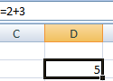
Чтобы задать формулу для ячейки, необходимо активизировать ее (поставить курсор) и ввести равно (=). Так же можно вводить знак равенства в строку формул. После введения формулы нажать Enter. В ячейке появится результат вычислений.

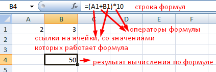
В Excel применяются стандартные математические операторы:

Оператор	Операция	Пример
+ (плюс)	Сложение	=В4+7
— (минус)	Вычитание	=А9-100
* (звездочка)	Умножение	=А3*2
/ (наклонная черта)	Деление	=А7/А8
^ (циркумфлекс)	Степень	=6^2
= (знак равенства)	Равно
<	Меньше
>	Больше
<=	Меньше или равно
>=	Больше или равно
<>	Не равно

Символ «*» используется обязательно при умножении. Опускать его, как принято во время письменных арифметических вычислений, недопустимо. То есть запись (2+3)5 Excel не поймет.

Программу Excel можно использовать как калькулятор. То есть вводить в формулу числа и операторы математических вычислений и сразу получать результат.

Но чаще вводятся адреса ячеек. То есть пользователь вводит ссылку на ячейку, со значением которой будет оперировать формула.

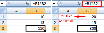
При изменении значений в ячейках формула автоматически пересчитывает результат.

Ссылки можно комбинировать в рамках одной формулы с простыми числами.

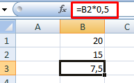
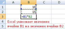
Оператор умножил значение ячейки В2 на 0,5. Чтобы ввести в формулу ссылку на ячейку, достаточно щелкнуть по этой ячейке.

В нашем примере:

Поставили курсор в ячейку В3 и ввели =.
Щелкнули по ячейке В2 – Excel «обозначил» ее (имя ячейки появилось в формуле, вокруг ячейки образовался «мелькающий» прямоугольник).
Ввели знак *, значение 0,5 с клавиатуры и нажали ВВОД.

Если в одной формуле применяется несколько операторов, то программа обработает их в следующей последовательности:

%, ^;
*, /;
+, -.

Поменять последовательность можно посредством круглых скобок: Excel в первую очередь вычисляет значение выражения в скобках.

Как в формуле Excel обозначить постоянную ячейку

Различают два вида ссылок на ячейки: относительные и абсолютные. При копировании формулы эти ссылки ведут себя по-разному: относительные изменяются, абсолютные остаются постоянными.

Все ссылки на ячейки программа считает относительными, если пользователем не задано другое условие. С помощью относительных ссылок можно размножить одну и ту же формулу на несколько строк или столбцов.

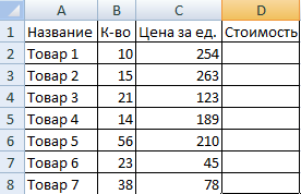
Вручную заполним первые графы учебной таблицы. У нас – такой вариант:

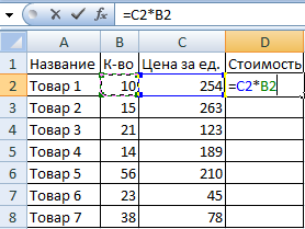
Вспомним из математики: чтобы найти стоимость нескольких единиц товара, нужно цену за 1 единицу умножить на количество. Для вычисления стоимости введем формулу в ячейку D2: = цена за единицу * количество. Константы формулы – ссылки на ячейки с соответствующими значениями.

Нажимаем ВВОД – программа отображает значение умножения. Те же манипуляции необходимо произвести для всех ячеек. Как в Excel задать формулу для столбца: копируем формулу из первой ячейки в другие строки. Относительные ссылки – в помощь.

Находим в правом нижнем углу первой ячейки столбца маркер автозаполнения. Нажимаем на эту точку левой кнопкой мыши, держим ее и «тащим» вниз по столбцу.

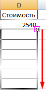
Отпускаем кнопку мыши – формула скопируется в выбранные ячейки с относительными ссылками. То есть в каждой ячейке будет своя формула со своими аргументами.

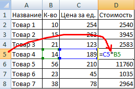
Ссылки в ячейке соотнесены со строкой.

Формула с абсолютной ссылкой ссылается на одну и ту же ячейку. То есть при автозаполнении или копировании константа остается неизменной (или постоянной).

Чтобы указать Excel на абсолютную ссылку, пользователю необходимо поставить знак доллара ($). Проще всего это сделать с помощью клавиши F4.

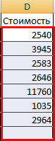
Создадим строку «Итого». Найдем общую стоимость всех товаров. Выделяем числовые значения столбца «Стоимость» плюс еще одну ячейку. Это диапазон D2:D9

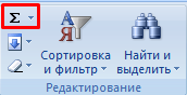
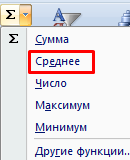
Воспользуемся функцией автозаполнения. Кнопка находится на вкладке «Главная» в группе инструментов «Редактирование».

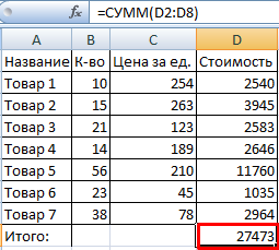
После нажатия на значок «Сумма» (или комбинации клавиш ALT+«=») слаживаются выделенные числа и отображается результат в пустой ячейке.

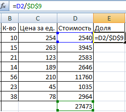
Сделаем еще один столбец, где рассчитаем долю каждого товара в общей стоимости. Для этого нужно:

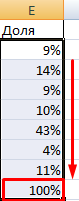
Разделить стоимость одного товара на стоимость всех товаров и результат умножить на 100. Ссылка на ячейку со значением общей стоимости должна быть абсолютной, чтобы при копировании она оставалась неизменной.

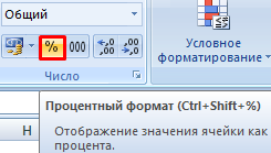
Чтобы получить проценты в Excel, не обязательно умножать частное на 100. Выделяем ячейку с результатом и нажимаем «Процентный формат». Или нажимаем комбинацию горячих клавиш: CTRL+SHIFT+5

Копируем формулу на весь столбец: меняется только первое значение в формуле (относительная ссылка). Второе (абсолютная ссылка) остается прежним. Проверим правильность вычислений – найдем итог. 100%. Все правильно.

При создании формул используются следующие форматы абсолютных ссылок:

$В$2 – при копировании остаются постоянными столбец и строка;
B$2 – при копировании неизменна строка;
$B2 – столбец не изменяется.

Как составить таблицу в Excel с формулами

Чтобы сэкономить время при введении однотипных формул в ячейки таблицы, применяются маркеры автозаполнения. Если нужно закрепить ссылку, делаем ее абсолютной. Для изменения значений при копировании относительной ссылки.

Простейшие формулы заполнения таблиц в Excel:

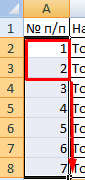
Перед наименованиями товаров вставим еще один столбец. Выделяем любую ячейку в первой графе, щелкаем правой кнопкой мыши. Нажимаем «Вставить». Или жмем сначала комбинацию клавиш: CTRL+ПРОБЕЛ, чтобы выделить весь столбец листа. А потом комбинация: CTRL+SHIFT+»=», чтобы вставить столбец.
Назовем новую графу «№ п/п». Вводим в первую ячейку «1», во вторую – «2». Выделяем первые две ячейки – «цепляем» левой кнопкой мыши маркер автозаполнения – тянем вниз.

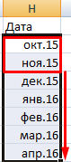
По такому же принципу можно заполнить, например, даты. Если промежутки между ними одинаковые – день, месяц, год. Введем в первую ячейку «окт.15», во вторую – «ноя.15». Выделим первые две ячейки и «протянем» за маркер вниз.

Найдем среднюю цену товаров. Выделяем столбец с ценами + еще одну ячейку. Открываем меню кнопки «Сумма» — выбираем формулу для автоматического расчета среднего значения.

Чтобы проверить правильность вставленной формулы, дважды щелкните по ячейке с результатом.

Источник

Формулы Excel используют, когда данных очень много. Например, чтобы посчитать сумму нескольких чисел быстрее, чем на калькуляторе. Преимуществ много, поэтому работодатели часто указывают эту программу в требованиях. В конце марта 2022 года 64 225 вакансий на хедхантере содержали формулировки вроде «уверенный пользователь Excel», «работа с формулами в Excel».

Кому важно знать Excel и где выучить основы

Excel нужен бухгалтерам, чтобы вести учет в таблицах. Экономистам, чтобы делать перерасчет цен, анализировать показатели компании. Менеджерам — вести базу клиентов. Аналитикам — строить и проверять гипотезы.

Программу можно освоить самостоятельно, например по статьям в интернете. Но это поможет понять только основные формулы. Если нужны глубокие знания — как строить сложные прогнозы, собирать калькулятор юнит-экономики, — пройдите курсы.

Аналитик данных: новая работа через 5 месяцев

Получится, даже если у вас нет опыта в IT

Узнать больше

На онлайн-курсе Skypro «Аналитик данных» научитесь владеть базовыми формулами Excel, работать с нестандартными данными, статистикой. Кроме Excel вы изучите Metabase, SQL, Power BI, язык программирования Python. Программа подойдет даже тем, у кого совсем нет опыта в анализе и кто не любит математику. Вас ждут живые вебинары, мастер-классы, домашки с разбором, помощь наставников.

Урок из курса «Аналитик данных» в Skypro

Из чего состоит формула в Excel

Основные знаки:

= с него начинают любую формулу;

( ) заключают формулу и ее части;

; применяют, чтобы указать очередность ячеек или действий;

: ставят, чтобы обозначить диапазон ячеек, а не выбирать всё подряд вручную.

В Excel работают с простыми математическими действиями:

сложением +

вычитанием —

умножением *

делением /

возведением в степень ^

Еще используют символы сравнения:

равенство =

меньше <

больше >

меньше либо равно <=

больше либо равно >=

не равно <>

Основные виды

Все формулы в Excel делятся на простые, сложные и комбинированные. Их можно написать самостоятельно или воспользоваться встроенными.

Простые

Применяют, когда нужно совершить одно простое действие, например сложить или умножить.

✅ СУММ. Складывает несколько чисел. Сумму можно посчитать для нескольких ячеек или целого диапазона.

=СУММ(А1;В1) — для соседних ячеек;

=СУММ(А1;С1;H1) — для определенных ячеек;

=СУММ(А1:Е1) — для диапазона.

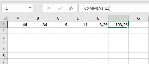
Сумма всех чисел в ячейках от А1 до Е1

✅ ПРОИЗВЕД. Умножает числа в соседних, выбранных вручную ячейках или диапазоне.

=ПРОИЗВЕД(А1;В1)

=ПРОИЗВЕД(А1;С1;H1)

=ПРОИЗВЕД(А1:Е1)

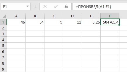
Произведение всех чисел в ячейках от А1 до Е1

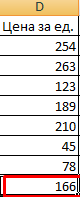
✅ ОКРУГЛ. Округляет дробное число до целого в большую или меньшую сторону. Укажите ячейку с нужным числом, в качестве второго значения — 0.

=ОКРУГЛВВЕРХ(А1;0) — к большему целому числу;

=ОКРУГЛВНИЗ(А1;0) — к меньшему.

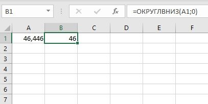
Округление в меньшую сторону

✅ ВПР. Находит данные в таблице или определенном диапазоне.

=ВПР(С1;А1:В6;2)

С1 — ячейка, в которую выписывают известные данные. В примере это код цвета.
А1 по В6 — диапазон ячеек. Ищем название цвета по коду.
2 — порядковый номер столбца для поиска. В нём указаны названия цвета.

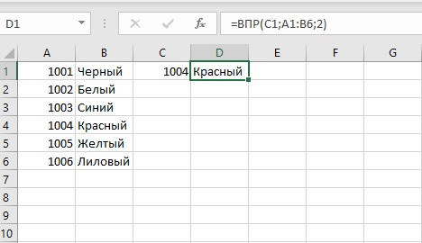
Формула вычислила, какой цвет соответствует коду

✅ СЦЕПИТЬ. Объединяет данные диапазона ячеек, например текст или цифры. Между содержимым ячеек можно добавить пробел, если объединяете слова в предложения.

=СЦЕПИТЬ(А1;В1;С1) — текст без пробелов;

=СЦЕПИТЬ(А1;» «;В1;» «С1) — с пробелами.

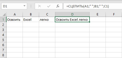
Формула объединила три слова в одно предложение

✅ КОРЕНЬ. Вычисляет квадратный корень числа в ячейке.

=КОРЕНЬ(А1)

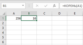
Квадратный корень числа в ячейке А1

✅ ПРОПИСН. Преобразует текст в верхний регистр, то есть делает буквы заглавными.

=ПРОПИСН(А1:С1)

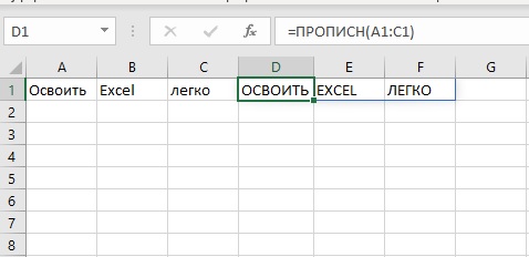
Формула преобразовала строчные буквы в прописные

✅ СТРОЧН. Переводит текст в нижний регистр, то есть делает из больших букв маленькие.

=СТРОЧН(А2)

✅ СЧЕТ. Считает количество ячеек с числами.

=СЧЕТ(А1:В5)

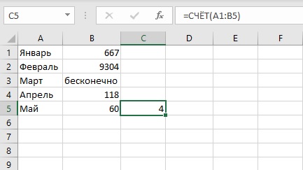
Формула вычислила, что в диапазоне А1:В5 четыре ячейки с числами

✅ СЖПРОБЕЛЫ. Убирает лишние пробелы. Например, когда переносите текст из другого документа и сомневаетесь, правильно ли там стоят пробелы.

=СЖПРОБЕЛЫ(А1)

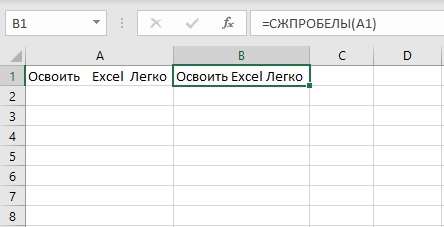
Формула удалила двойные и тройные пробелы

Сложные

✅ ПСТР. Выделяет определенное количество знаков в тексте, например одно слово.

=ПСТР(А1;9;5)

Введите =ПСТР.
Кликните на ячейку, где нужно выделить знаки.
Укажите номер начального знака: например, с какого символа начинается слово. Пробелы тоже считайте.
Поставьте количество знаков, которые нужно выделить из текста. Например, если слово состоит из пяти букв, впишите цифру 5.

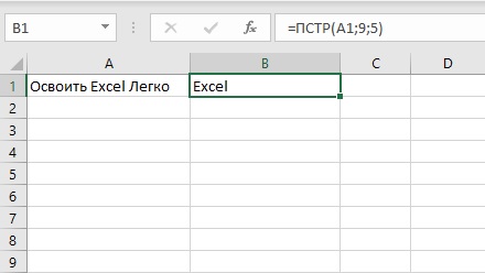
В ячейке А1 формула выделила 5 символов, начиная с 9-го

✅ ЕСЛИ. Анализирует данные по условию. Например, когда нужно сравнить одно с другим.

=ЕСЛИ(A1>25;"больше 25";"меньше или равно 25")

В формуле указали:

А1 — ячейку с данными;
>25 — логическое выражение;
больше 25, меньше или равно 25 — истинное и ложное значения.

Первый результат возвращается, если сравнение истинно. Второй — если ложно.

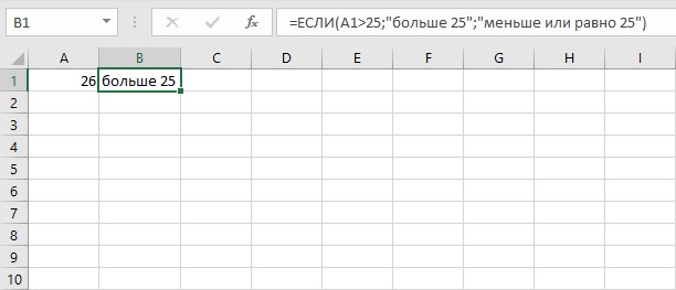
Число в А1 больше 25. Поэтому формула показывает первый результат — больше 25.

✅ СУММЕСЛИ. Складывает числа, которые соответствуют критерию. Обычно критерий — числовой промежуток или предел.

=СУММЕСЛИ(В2:В5;">10")

В формуле указали:

В2:В5 — диапазон ячеек;
>10 — критерий, то есть числа меньше 10 не будут суммироваться.

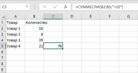
Число 8 меньше указанного в условии, то есть 10. Поэтому оно не вошло в сумму.

✅ СУММЕСЛИМН. Складывает числа, когда условий несколько. В формуле указывают диапазоны — ячейки, которые нужно учитывать. И условия — содержание подходящих ячеек. Например:

=СУММЕСЛИМН(D2:D6;C2:C6;"сувениры";B2:B6;"ООО ХY")

D2:D6 — диапазон, из которого суммируем числа;
C2:C6 — диапазон ячеек для категории;
сувениры — условие, то есть числа другой категории учитываться не будут;
B2:B6 — диапазон ячеек для компании;
ООО XY — условие, то есть числа другой компании учитываться не будут.

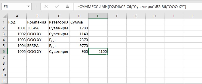
Под условия подошли только ячейки D3 и D6: их сумму и вывела формула

Комбинированные

В Excel можно комбинировать несколько функций: сложение, умножение, сравнение и другие. Например, вам нужно найти сумму двух чисел. Если значение больше 65, сумму нужно умножить на 1,5. Если меньше — на 2.

=ЕСЛИ(СУММ(A1;B1)<65;СУММ(A1;B1)*1,5;(СУММ(A1;B1)*2))

То есть если сумма двух чисел в А1 и В1 окажется меньше 65, программа посчитает первое условие — СУММ(А1;В1)*1,5. Больше 65 — Excel задействует второе условие — СУММ(А1;В1)*2.

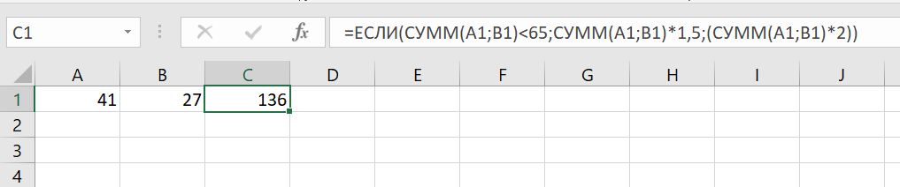
Сумма в А1 и В1 больше 65, поэтому формула посчитала по второму условию: умножила на 2

Встроенные

Используйте их, если удобнее пользоваться готовыми формулами, а не вписывать вручную.

Поместите курсор в нужную ячейку.
Откройте диалоговое окно мастера: нажмите клавиши Shift + F3. Откроется список функций.
Выберите нужную формулу. Нажмите на нее, затем на «ОК». Откроется окно «Аргументы функций».
Внесите нужные данные. Например, числа, которые нужно сложить.

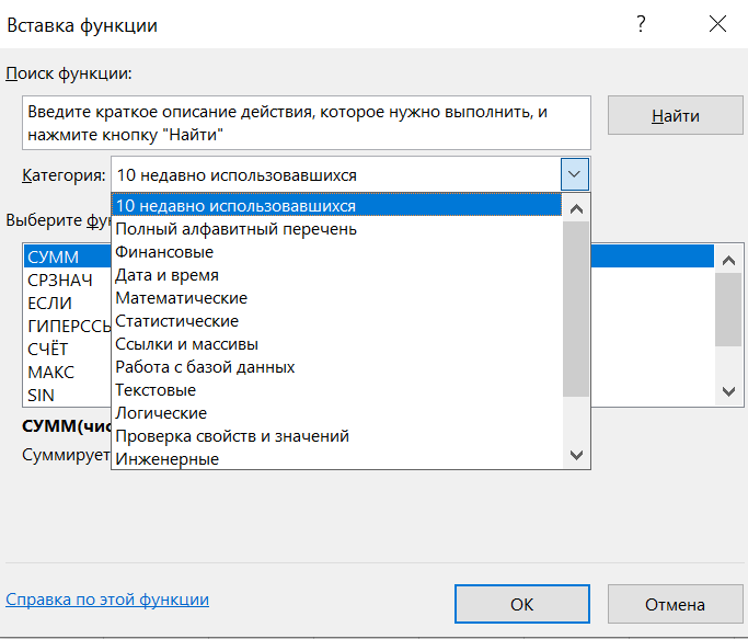
Ищите формулу по алфавиту или тематике, выбирайте любую из тех, что использовали недавно

Как скопировать

Если для разных ячеек нужны однотипные действия, например сложить числа не в одной, а в нескольких строках, скопируйте формулу.

Впишите функцию в ячейку и кликните на нее.
Наведите курсор на правый нижний угол — курсор примет форму креста.
Нажмите левую кнопку мыши, удерживайте ее и тяните до нужной ячейки.
Отпустите кнопку. Появится итог.

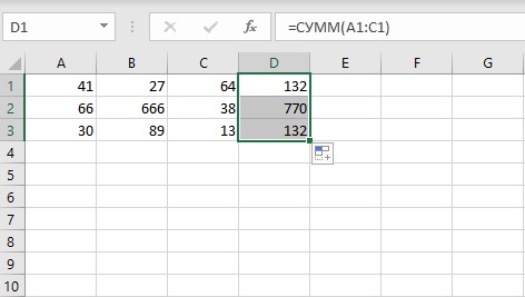
Посчитали сумму ячеек в трех строках

Как обозначить постоянную ячейку

Это нужно, чтобы, когда вы протягивали формулу, ссылка на ячейку не смещалась.

Нажмите на ячейку с формулой.
Поместите курсор в нужную ячейку и нажмите F4.
В формуле фрагмент с описанием ячейки приобретет вид $A$1. Если вы протянете формулу, то ссылка на ячейку $A$1 останется на месте.

Как поставить «плюс», «равно» без формулы

Когда нужна не формула, а данные, например +10 °С:

Кликните правой кнопкой по ячейке.
Выберите «Формат ячеек».
Отметьте «Текстовый», нажмите «ОК».
Поставьте = или +, затем нужное число.
Нажмите Enter.

Главное о формулах в Excel

Формула состоит из математических знаков. Чтобы ее вписать, используют символы = ( ) ; : .
С помощью простых формул числа складывают, умножают, округляют, извлекают из них квадратный корень. Чтобы отредактировать текст, используют формулы поиска, изменения регистра, удаления лишних пробелов.
Сложные и комбинированные формулы помогают делать объемные вычисления, когда нужно соблюдать несколько условий.

Источник

MS Excel: Formulas and Functions — Listed by Category

Learn how to use all 300+ Excel formulas and functions including worksheet functions entered in the formula bar and VBA functions used in Macros.

Worksheet formulas are built-in functions that are entered as part of a formula in a cell. These are the most basic functions used when learning Excel. VBA functions are built-in functions that are used in Excel’s programming environment called Visual Basic for Applications (VBA).

Below is a list of Excel formulas sorted by category. If you would like an alphabetical list of these formulas, click on the following button:

Sort Alphabetically

(Enter a value in the field above to quickly find functions in the list below)

Lookup/Ref Functions

ADDRESS (WS)	Returns a text representation of a cell address
AREAS (WS)	Returns the number of ranges in a reference
CHOOSE (WS, VBA)	Returns a value from a list of values based on a given position
COLUMN (WS)	Returns the column number of a cell reference
COLUMNS (WS)	Returns the number of columns in a cell reference
HLOOKUP (WS)	Performs a horizontal lookup by searching for a value in the top row of the table and returning the value in the same column based on the index_number
HYPERLINK (WS)	Creates a shortcut to a file or Internet address
INDEX (WS)	Returns either the value or the reference to a value from a table or range
INDIRECT (WS)	Returns the reference to a cell based on its string representation
LOOKUP (WS)	Returns a value from a range (one row or one column) or from an array
MATCH (WS)	Searches for a value in an array and returns the relative position of that item
OFFSET (WS)	Returns a reference to a range that is offset a number of rows and columns
ROW (WS)	Returns the row number of a cell reference
ROWS (WS)	Returns the number of rows in a cell reference
TRANSPOSE (WS)	Returns a transposed range of cells
VLOOKUP (WS)	Performs a vertical lookup by searching for a value in the first column of a table and returning the value in the same row in the index_number position
XLOOKUP (WS)	Performs a lookup (either vertical or horizontal)

String/Text Functions

ASC (VBA)	Returns ASCII value of a character
BAHTTEXT (WS)	Returns the number in Thai text
CHAR (WS)	Returns the character based on the ASCII value
CHR (VBA)	Returns the character based on the ASCII value
CLEAN (WS)	Removes all nonprintable characters from a string
CODE (WS)	Returns the ASCII value of a character or the first character in a cell
CONCAT (WS)	Used to join 2 or more strings together
CONCATENATE (WS)	Used to join 2 or more strings together (replaced by CONCAT Function)
CONCATENATE with & (WS, VBA)	Used to join 2 or more strings together using the & operator
DOLLAR (WS)	Converts a number to text, using a currency format
EXACT (WS)	Compares two strings and returns TRUE if both values are the same
FIND (WS)	Returns the location of a substring in a string (case-sensitive)
FIXED (WS)	Returns a text representation of a number rounded to a specified number of decimal places
FORMAT STRINGS (VBA)	Takes a string expression and returns it as a formatted string
INSTR (VBA)	Returns the position of the first occurrence of a substring in a string
INSTRREV (VBA)	Returns the position of the first occurrence of a string in another string, starting from the end of the string
LCASE (VBA)	Converts a string to lowercase
LEFT (WS, VBA)	Extract a substring from a string, starting from the left-most character
LEN (WS, VBA)	Returns the length of the specified string
LOWER (WS)	Converts all letters in the specified string to lowercase
LTRIM (VBA)	Removes leading spaces from a string
MID (WS, VBA)	Extracts a substring from a string (starting at any position)
NUMBERVALUE (WS)	Returns a text to a number specifying the decimal and group separators
PROPER (WS)	Sets the first character in each word to uppercase and the rest to lowercase
REPLACE (WS)	Replaces a sequence of characters in a string with another set of characters
REPLACE (VBA)	Replaces a sequence of characters in a string with another set of characters
REPT (WS)	Returns a repeated text value a specified number of times
RIGHT (WS, VBA)	Extracts a substring from a string starting from the right-most character
RTRIM (VBA)	Removes trailing spaces from a string
SEARCH (WS)	Returns the location of a substring in a string
SPACE (VBA)	Returns a string with a specified number of spaces
SPLIT (VBA)	Used to split a string into substrings based on a delimiter
STR (VBA)	Returns a string representation of a number
STRCOMP (VBA)	Returns an integer value representing the result of a string comparison
STRCONV (VBA)	Returns a string converted to uppercase, lowercase, proper case or Unicode
STRREVERSE (VBA)	Returns a string whose characters are in reverse order
SUBSTITUTE (WS)	Replaces a set of characters with another
T (WS)	Returns the text referred to by a value
TEXT (WS)	Returns a value converted to text with a specified format
TEXTJOIN (WS)	Used to join 2 or more strings together separated by a delimiter
TRIM (WS, VBA)	Returns a text value with the leading and trailing spaces removed
UCASE (VBA)	Converts a string to all uppercase
UNICHAR (WS)	Returns the Unicode character based on the Unicode number provided
UNICODE (WS)	Returns the Unicode number of a character or the first character in a string
UPPER (WS)	Convert text to all uppercase
VAL (VBA)	Returns the numbers found in a string
VALUE (WS)	Converts a text value that represents a number to a number

Date/Time Functions

DATE (WS)	Returns the serial date value for a date
DATE (VBA)	Returns the current system date
DATEADD (VBA)	Returns a date after which a certain time/date interval has been added
DATEDIF (WS)	Returns the difference between two date values, based on the interval specified
DATEDIFF (VBA)	Returns the difference between two date values, based on the interval specified
DATEPART (VBA)	Returns a specified part of a given date
DATESERIAL (VBA)	Returns a date given a year, month, and day value
DATEVALUE (WS, VBA)	Returns the serial number of a date
DAY (WS, VBA)	Returns the day of the month (a number from 1 to 31) given a date value
DAYS (WS)	Returns the number of days between 2 dates
DAYS360 (WS)	Returns the number of days between two dates based on a 360-day year
EDATE (WS)	Adds a specified number of months to a date and returns the result as a serial date
EOMONTH (WS)	Calculates the last day of the month after adding a specified number of months to a date
FORMAT DATES (VBA)	Takes a date expression and returns it as a formatted string
HOUR (WS, VBA)	Returns the hours (a number from 0 to 23) from a time value
ISOWEEKNUM (WS)	Returns the ISO week number for a date
MINUTE (WS, VBA)	Returns the minutes (a number from 0 to 59) from a time value
MONTH (WS, VBA)	Returns the month (a number from 1 to 12) given a date value
MONTHNAME (VBA)	Returns a string representing the month given a number from 1 to 12
NETWORKDAYS (WS)	Returns the number of work days between 2 dates, excluding weekends and holidays
NETWORKDAYS.INTL (WS)	Returns the number of work days between 2 dates, excluding weekends and holidays
NOW (WS, VBA)	Returns the current system date and time
SECOND (WS)	Returns the seconds (a number from 0 to 59) from a time value
TIME (WS)	Returns a decimal number given an hour, minute and second value
TIMESERIAL (VBA)	Returns a time given an hour, minute, and second value
TIMEVALUE (WS, VBA)	Returns the serial number of a time
TODAY (WS)	Returns the current system date
WEEKDAY (WS, VBA)	Returns a number representing the day of the week, given a date value
WEEKDAYNAME (VBA)	Returns a string representing the day of the week given a number from 1 to 7
WEEKNUM (WS)	Returns the week number for a date
WORKDAY (WS)	Adds a specified number of work days to a date and returns the result as a serial date
WORKDAY.INTL (WS)	Adds a specified number of work days to a date and returns the result as a serial date (customizable weekends)
YEAR (WS, VBA)	Returns a four-digit year (a number from 1900 to 9999) given a date value
YEARFRAC (WS)	Returns the number of days between 2 dates as a year fraction

Math/Trig Functions

ABS (WS, VBA)	Returns the absolute value of a number
ACOS (WS)	Returns the arccosine (in radians) of a number
ACOSH (WS)	Returns the inverse hyperbolic cosine of a number
AGGREGATE (WS)	Apply functions such AVERAGE, SUM, COUNT, MAX or MIN and ignore errors or hidden rows
ASIN (WS)	Returns the arcsine (in radians) of a number
ASINH (WS)	Returns the inverse hyperbolic sine of a number
ATAN (WS)	Returns the arctangent (in radians) of a number
ATAN2 (WS)	Returns the arctangent (in radians) of (x,y) coordinates
ATANH (WS)	Returns the inverse hyperbolic tangent of a number
ATN (VBA)	Returns the arctangent of a number
CEILING (WS)	Returns a number rounded up based on a multiple of significance
CEILING.PRECISE (WS)	Returns a number rounded up to the nearest integer or to the nearest multiple of significance
COMBIN (WS)	Returns the number of combinations for a specified number of items
COMBINA (WS)	Returns the number of combinations for a specified number of items and includes repetitions
COS (WS, VBA)	Returns the cosine of an angle
COSH (WS)	Returns the hyperbolic cosine of a number
DEGREES (WS)	Converts radians into degrees
EVEN (WS)	Rounds a number up to the nearest even integer
EXP (WS, VBA)	Returns e raised to the nth power
FACT (WS)	Returns the factorial of a number
FIX (VBA)	Returns the integer portion of a number
FLOOR (WS)	Returns a number rounded down based on a multiple of significance
FORMAT NUMBERS (VBA)	Takes a numeric expression and returns it as a formatted string
INT (WS, VBA)	Returns the integer portion of a number
LN (WS)	Returns the natural logarithm of a number
LOG (WS)	Returns the logarithm of a number to a specified base
LOG (VBA)	Returns the natural logarithm of a number
LOG10 (WS)	Returns the base-10 logarithm of a number
MDETERM (WS)	Returns the matrix determinant of an array
MINVERSE (WS)	Returns the inverse matrix for a given matrix
MMULT (WS)	Returns the matrix product of two arrays
MOD (WS)	Returns the remainder after a number is divided by a divisor
MOD (VBA)	Returns the remainder after a number is divided by a divisor
ODD (WS)	Rounds a number up to the nearest odd integer
PI (WS)	Returns the mathematical constant called pi
POWER (WS)	Returns the result of a number raised to a given power
PRODUCT (WS)	Multiplies the numbers and returns the product
RADIANS (WS)	Converts degrees into radians
RAND (WS)	Returns a random number that is greater than or equal to 0 and less than 1
RANDBETWEEN (WS)	Returns a random number that is between a bottom and top range
RANDOMIZE (VBA)	Used to change the seed value used by the random number generator for the RND function
RND (VBA)	Used to generate a random number (integer value)
ROMAN (WS)	Converts a number to roman numeral
ROUND (WS)	Returns a number rounded to a specified number of digits
ROUND (VBA)	Returns a number rounded to a specified number of digits
ROUNDDOWN (WS)	Returns a number rounded down to a specified number of digits
ROUNDUP (WS)	Returns a number rounded up to a specified number of digits
SGN (VBA)	Returns the sign of a number
SIGN (WS)	Returns the sign of a number
SIN (WS, VBA)	Returns the sine of an angle
SINH (WS)	Returns the hyperbolic sine of a number
SQR (VBA)	Returns the square root of a number
SQRT (WS)	Returns the square root of a number
SUBTOTAL (WS)	Returns the subtotal of the numbers in a column in a list or database
SUM (WS)	Adds all numbers in a range of cells
SUMIF (WS)	Adds all numbers in a range of cells based on one criteria
SUMIFS (WS)	Adds all numbers in a range of cells, based on a single or multiple criteria
SUMPRODUCT (WS)	Multiplies the corresponding items in the arrays and returns the sum of the results
SUMSQ (WS)	Returns the sum of the squares of a series of values
SUMX2MY2 (WS)	Returns the sum of the difference of squares between two arrays
SUMX2PY2 (WS)	Returns the sum of the squares of corresponding items in the arrays
SUMXMY2 (WS)	Returns the sum of the squares of the differences between corresponding items in the arrays
TAN (WS, VBA)	Returns the tangent of an angle
TANH (WS)	Returns the hyperbolic tangent of a number
TRUNC (WS)	Returns a number truncated to a specified number of digits

Statistical Functions

AVEDEV (WS)	Returns the average of the absolute deviations of the numbers provided
AVERAGE (WS)	Returns the average of the numbers provided
AVERAGEA (WS)	Returns the average of the numbers provided and treats TRUE as 1 and FALSE as 0
AVERAGEIF (WS)	Returns the average of all numbers in a range of cells, based on a given criteria
AVERAGEIFS (WS)	Returns the average of all numbers in a range of cells, based on multiple criteria
BETA.DIST (WS)	Returns the beta distribution
BETA.INV (WS)	Returns the inverse of the cumulative beta probability density function
BETADIST (WS)	Returns the cumulative beta probability density function
BETAINV (WS)	Returns the inverse of the cumulative beta probability density function
BINOM.DIST (WS)	Returns the individual term binomial distribution probability
BINOM.INV (WS)	Returns the smallest value for which the cumulative binomial distribution is greater than or equal to a criterion
BINOMDIST (WS)	Returns the individual term binomial distribution probability
CHIDIST (WS)	Returns the one-tailed probability of the chi-squared distribution
CHIINV (WS)	Returns the inverse of the one-tailed probability of the chi-squared distribution
CHITEST (WS)	Returns the value from the chi-squared distribution
COUNT (WS)	Counts the number of cells that contain numbers as well as the number of arguments that contain numbers
COUNTA (WS)	Counts the number of cells that are not empty as well as the number of value arguments provided
COUNTBLANK (WS)	Counts the number of empty cells in a range
COUNTIF (WS)	Counts the number of cells in a range, that meets a given criteria
COUNTIFS (WS)	Counts the number of cells in a range, that meets a single or multiple criteria
COVAR (WS)	Returns the covariance, the average of the products of deviations for two data sets
FORECAST (WS)	Returns a prediction of a future value based on existing values provided
FREQUENCY (WS)	Returns how often values occur within a set of data. It returns a vertical array of numbers
GROWTH (WS)	Returns the predicted exponential growth based on existing values provided
INTERCEPT (WS)	Returns the y-axis intersection point of a line using x-axis values and y-axis values
LARGE (WS)	Returns the nth largest value from a set of values
LINEST (WS)	Uses the least squares method to calculate the statistics for a straight line and returns an array describing that line
MAX (WS)	Returns the largest value from the numbers provided
MAXA (WS)	Returns the largest value from the values provided (numbers, text and logical values)
MAXIFS (WS)	Returns the largest value in a range, that meets a single or multiple criteria
MEDIAN (WS)	Returns the median of the numbers provided
MIN (WS)	Returns the smallest value from the numbers provided
MINA (WS)	Returns the smallest value from the values provided (numbers, text and logical values)
MINIFS (WS)	Returns the smallest value in a range, that meets a single or multiple criteria
MODE (WS)	Returns most frequently occurring number
MODE.MULT (WS)	Returns a vertical array of the most frequently occurring numbers
MODE.SNGL (WS)	Returns most frequently occurring number
PERCENTILE (WS)	Returns the nth percentile from a set of values
PERCENTRANK (WS)	Returns the nth percentile from a set of values
PERMUT (WS)	Returns the number of permutations for a specified number of items
QUARTILE (WS)	Returns the quartile from a set of values
RANK (WS)	Returns the rank of a number within a set of numbers
SLOPE (WS)	Returns the slope of a regression line based on the data points identified by known_y_values and known_x_values
SMALL (WS)	Returns the nth smallest value from a set of values
STDEV (WS)	Returns the standard deviation of a population based on a sample of numbers
STDEVA (WS)	Returns the standard deviation of a population based on a sample of numbers, text, and logical values
STDEVP (WS)	Returns the standard deviation of a population based on an entire population of numbers
STDEVPA (WS)	Returns the standard deviation of a population based on an entire population of numbers, text, and logical values
VAR (WS)	Returns the variance of a population based on a sample of numbers
VARA (WS)	Returns the variance of a population based on a sample of numbers, text, and logical values
VARP (WS)	Returns the variance of a population based on an entire population of numbers
VARPA (WS)	Returns the variance of a population based on an entire population of numbers, text, and logical values

Logical Functions

AND (WS)	Returns TRUE if all conditions are TRUE
AND (VBA)	Returns TRUE if all conditions are TRUE
CASE (VBA)	Has the functionality of an IF-THEN-ELSE statement
FALSE (WS)	Returns a logical value of FALSE
FOR…NEXT (VBA)	Used to create a FOR LOOP
IF (WS)	Returns one value if the condition is TRUE or another value if the condition is FALSE
IF (more than 7) (WS)	Nest more than 7 IF functions
IF (up to 7) (WS)	Nest up to 7 IF functions
IF-THEN-ELSE (VBA)	Returns a value if a specified condition evaluates to TRUE or another value if it evaluates to FALSE
IFERROR (WS)	Used to return an alternate value if a formula results in an error
IFNA (WS)	Used to return an alternate value if a formula results in #N/A error
IFS (WS)	Specify multiple IF conditions within 1 function
NOT (WS)	Returns the reversed logical value
OR (WS)	Returns TRUE if any of the conditions are TRUE
OR (VBA)	Returns TRUE if any of the conditions are TRUE
SWITCH (WS)	Compares an expression to a list of values and returns the corresponding result
SWITCH (VBA)	Evaluates a list of expressions and returns the corresponding value for the first expression in the list that is TRUE
TRUE (WS)	Returns a logical value of TRUE
WHILE…WEND (VBA)	Used to create a WHILE LOOP

Information Functions

CELL (WS)	Used to retrieve information about a cell such as contents, formatting, size, etc.
ENVIRON (VBA)	Returns the value of an operating system environment variable
ERROR.TYPE (WS)	Returns the numeric representation of an Excel error
INFO (WS)	Returns information about the operating environment
ISBLANK (WS)	Used to check for blank or null values
ISDATE (VBA)	Returns TRUE if the expression is a valid date
ISEMPTY (VBA)	Used to check for blank cells or uninitialized variables
ISERR (WS)	Used to check for error values except #N/A
ISERROR (WS, VBA)	Used to check for error values
ISLOGICAL (WS)	Used to check for a logical value (TRUE or FALSE)
ISNA (WS)	Used to check for #N/A error
ISNONTEXT (WS)	Used to check for a value that is not text
ISNULL (VBA)	Used to check for a NULL value
ISNUMBER (WS)	Used to check for a numeric value
ISNUMERIC (VBA)	Used to check for a numeric value
ISREF (WS)	Used to check for a reference
ISTEXT (WS)	Used to check for a text value
N (WS)	Converts a value to a number
NA (WS)	Returns the #N/A error value
TYPE (WS)	Returns the type of a value

Financial Functions

ACCRINT (WS)	Returns the accrued interest for a security that pays interest on a periodic basis
ACCRINTM (WS)	Returns the accrued interest for a security that pays interest at maturity
AMORDEGRC (WS)	Returns the linear depreciation of an asset for each accounting period, on a prorated basis
AMORLINC (WS)	Returns the depreciation of an asset for each accounting period, on a prorated basis
DB (WS)	Returns the depreciation of an asset based on the fixed-declining balance method
DDB (WS, VBA)	Returns the depreciation of an asset based on the double-declining balance method
FV (WS, VBA)	Returns the future value of an investment
IPMT (WS, VBA)	Returns the interest payment for an investment
IRR (WS, VBA)	Returns the internal rate of return for a series of cash flows
ISPMT (WS)	Returns the interest payment for an investment
MIRR (WS, VBA)	Returns the modified internal rate of return for a series of cash flows
NPER (WS, VBA)	Returns the number of periods for an investment
NPV (WS, VBA)	Returns the net present value of an investment
PMT (WS, VBA)	Returns the payment amount for a loan
PPMT (WS, VBA)	Returns the payment on the principal for a particular payment
PV (WS, VBA)	Returns the present value of an investment
RATE (WS, VBA)	Returns the interest rate for an annuity
SLN (WS, VBA)	Returns the depreciation of an asset based on the straight-line depreciation method
SYD (WS, VBA)	Returns the depreciation of an asset based on the sum-of-years’ digits depreciation method
VDB (WS)	Returns the depreciation of an asset based on a variable declining balance depreciation method
XIRR (WS)	Returns the internal rate of return for a series of cash flows that may not be periodic

Database Functions

DAVERAGE (WS)	Averages all numbers in a column in a list or database, based on a given criteria
DCOUNT (WS)	Returns the number of cells in a column or database that contains numeric values and meets a given criteria
DCOUNTA (WS)	Returns the number of cells in a column or database that contains nonblank values and meets a given criteria
DGET (WS)	Retrieves from a database a single record that matches a given criteria
DMAX (WS)	Returns the largest number in a column in a list or database, based on a given criteria
DMIN (WS)	Returns the smallest number in a column in a list or database, based on a given criteria
DPRODUCT (WS)	Returns the product of the numbers in a column in a list or database, based on a given criteria
DSTDEV (WS)	Returns the standard deviation of a population based on a sample of numbers
DSTDEVP (WS)	Returns the standard deviation of a population based on the entire population of numbers
DSUM (WS)	Sums the numbers in a column or database that meets a given criteria
DVAR (WS)	Returns the variance of a population based on a sample of numbers
DVARP (WS)	Returns the variance of a population based on the entire population of numbers

Engineering Functions

BIN2DEC (WS)	Converts a binary number to a decimal number
BIN2HEX (WS)	Converts a binary number to a hexadecimal number
BIN2OCT (WS)	Converts a binary number to an octal number
COMPLEX (WS)	Converts coefficients (real and imaginary) into a complex number
CONVERT (WS)	Convert a number from one measurement unit to another measurement unit

File/Directory Functions

CHDIR (VBA)	Used to change the current directory or folder
CHDRIVE (VBA)	Used to change the current drive
CURDIR (VBA)	Returns the current path
DIR (VBA)	Returns the first filename that matches the pathname and attributes specified
FILEDATETIME (VBA)	Returns the date and time of when a file was created or last modified
FILELEN (VBA)	Returns the size of a file in bytes
GETATTR (VBA)	Returns an integer that represents the attributes of a file, folder, or directory
MKDIR (VBA)	Used to create a new folder or directory
SETATTR (VBA)	Used to set the attributes of a file

Data Type Conv. Functions

CBOOL (VBA)	Converts a value to a boolean
CBYTE (VBA)	Converts a value to a byte (ie: number between 0 and 255)
CCUR (VBA)	Converts a value to currency
CDATE (VBA)	Converts a value to a date
CDBL (VBA)	Converts a value to a double
CDEC (VBA)	Converts a value to a decimal number
CINT (VBA)	Converts a value to an integer
CLNG (VBA)	Converts a value to a long integer
CSNG (VBA)	Converts a value to a single-precision number
CSTR (VBA)	Converts a value to a string
CVAR (VBA)	Converts a value to a variant

More Lookup Functions

Other

Источник

Create a formula that refers to values in other cells

See a formula

Enter a formula that contains a built-in function

Download our Formulas tutorial workbook

Formulas in-depth

Need more help?

See Also

Need more help?

Want more options?

Создание формулы, ссылающейся на значения в других ячейках

Просмотр формулы

Ввод формулы, содержащей встроенную функцию

Скачивание книги «Учебник по формулам»

Подробные сведения о формулах

Дополнительные сведения

См. также

Нужна дополнительная помощь?

Формулы в Excel для чайников

Как в формуле Excel обозначить постоянную ячейку

Как составить таблицу в Excel с формулами

Кому важно знать Excel и где выучить основы

Из чего состоит формула в Excel

Основные виды

Простые

Сложные

Комбинированные

Встроенные

Как скопировать

Как обозначить постоянную ячейку

Как поставить «плюс», «равно» без формулы

Главное о формулах в Excel

MS Excel: Formulas and Functions — Listed by Category

Lookup/Ref Functions

String/Text Functions

Date/Time Functions

Math/Trig Functions

Statistical Functions

Logical Functions

Information Functions

Financial Functions

Database Functions

Engineering Functions

File/Directory Functions

Data Type Conv. Functions

More Lookup Functions

Other