Office excel if function - Word и Excel - помощь в работе с программами

IF function

The IF function is one of the most popular functions in Excel, and it allows you to make logical comparisons between a value and what you expect.

So an IF statement can have two results. The first result is if your comparison is True, the second if your comparison is False.

For example, =IF(C2=”Yes”,1,2) says IF(C2 = Yes, then return a 1, otherwise return a 2).

Use the IF function, one of the logical functions, to return one value if a condition is true and another value if it’s false.

IF(logical_test, value_if_true, [value_if_false])

For example:

=IF(A2>B2,»Over Budget»,»OK»)
=IF(A2=B2,B4-A4,»»)

Argument name	Description
logical_test (required)	The condition you want to test.
value_if_true (required)	The value that you want returned if the result of *logical_test* is TRUE.
value_if_false (optional)	The value that you want returned if the result of *logical_test* is FALSE.

Simple IF examples

=IF(C2=”Yes”,1,2)

In the above example, cell D2 says: IF(C2 = Yes, then return a 1, otherwise return a 2)

=IF(C2=1,”Yes”,”No”)

In this example, the formula in cell D2 says: IF(C2 = 1, then return Yes, otherwise return No)As you see, the IF function can be used to evaluate both text and values. It can also be used to evaluate errors. You are not limited to only checking if one thing is equal to another and returning a single result, you can also use mathematical operators and perform additional calculations depending on your criteria. You can also nest multiple IF functions together in order to perform multiple comparisons.

=IF(C2>B2,”Over Budget”,”Within Budget”)

In the above example, the IF function in D2 is saying IF(C2 Is Greater Than B2, then return “Over Budget”, otherwise return “Within Budget”)

=IF(C2>B2,C2-B2,0)

In the above illustration, instead of returning a text result, we are going to return a mathematical calculation. So the formula in E2 is saying IF(Actual is Greater than Budgeted, then Subtract the Budgeted amount from the Actual amount, otherwise return nothing).

=IF(E7=”Yes”,F5*0.0825,0)

In this example, the formula in F7 is saying IF(E7 = “Yes”, then calculate the Total Amount in F5 * 8.25%, otherwise no Sales Tax is due so return 0)

Note: If you are going to use text in formulas, you need to wrap the text in quotes (e.g. “Text”). The only exception to that is using TRUE or FALSE, which Excel automatically understands.

Common problems

Problem	What went wrong
0 (zero) in cell	There was no argument for either value_if_true or value_if_False arguments. To see the right value returned, add argument text to the two arguments, or add TRUE or FALSE to the argument.
#NAME? in cell	This usually means that the formula is misspelled.

Need more help?

You can always ask an expert in the Excel Tech Community or get support in the Answers community.

The syntax of the function «IF» with one condition

The operation syntax in Excel is the structure of the functions necessary for its operation data.

=IF(boolean;value_if_TRUE;value_if_FALSE)

Let us consider the function syntax:

Boolean – what the operator checks (text or numeric data cell).
Value_if_TRUE – what will appear in the cell when the text or numbers correspond to a predetermined condition (true).
Value_if_FALSE – what appears in the box when the text or the number does not meet the predetermined condition (false).

Example:

Logical IF functions.

The operator checks the A1 cell and compares it to 20. This is a «Boolean». When the contents of the column is more than 20, there is a true legend «greater 20». In the other case it’s «less or equal 20».

Attention! The words in the formula need to be quoted. For Excel to understand that you want to display text values.

Here is one more example. To gain admission to the exam, a group of students must successfully pass a test. The results are listed in a table with columns: a list of students, a credit, an exam.

list.

The statement IF should check not the digital data type but the text. Therefore, we prescribed in the formula В2= «done» We take the quotes for the program to recognize the text correctly.

The function IF in Excel with multiple conditions

Usually one condition for the logic function is not enough. If you need to consider several options for decision-making, spread operators’ IF into each other. Thus, we get several functions IF in Excel.

The syntax is as follows:

Here the operator checks the two parameters. If the first condition is true, the formula returns the first argument is the truth. False — the operator checks the second condition.

Examples of a few conditions of the function IF in Excel:

It’s a table for the analysis of the progress. The student received 5 points:

А – excellent;
В – above average or superior work;
C – satisfactory;
D – a passing grade;
E – completely unsatisfactory.

IF statement checks two conditions: the equality of value in the cells.

In this example, we have added a third condition, which implies the presence of another report card and «twos». The principle of the operator is the same.

Enhanced functionality with the help of the operators «AND» and «OR»

When you need to check out a few of the true conditions you use the function И. The point is: IF A = 1 AND A = 2 THEN meaning в ELSE meaning с.

OR function checks the condition 1 or condition 2. As soon as at least one condition is true, the result is true. The point is: IF A = 1 OR A = 2 THEN value B ELSE value C.

Functions AND & OR can check up to 30 conditions.

An example of using the operator AND:

It’s the example of using the logical operator OR.

How to compare data in two tables

Users often need to compare the two spreadsheets in an Excel to match. Examples of the «life»: compare the prices of goods in different bringing, to compare balances (accounting reports) in a few months, the progress of pupils (students) of different classes, in different quarters, etc.

To compare the two tables in Excel, you can use the COUNTIFS statement. Consider the order of application functions.

For example, consider the two tables with the specifications of various food processors. We planned allocation of color differences. This problem in Excel solves the conditional formatting.

Baseline data (tables, which will work with):

tables.

Select the first table. Conditional Formatting — create a rule — use a formula to determine the formatted cells:

In the formula bar write: = COUNTIFS (comparable range; first cell of first table)=0. Comparing range is in the second table.

To drive the formula into the range, just select it first cell and the last. «= 0» means the search for the exact command (not approximate) values.

Choose the format and establish what changes in the cell formula in compliance. It’s better to do a color fill.

Select the second table. Conditional Formatting — create a rule — use the formula. Use the same operator (COUNTIFS). For the second table formula:

Download all examples in Excel

Now it is easy to compare the characteristics of the data in the table.

Источник

Функция ЕСЛИ в Excel – примеры использования

Очень распространенный вариант расчётов в Excel — «если — то». То есть, при выполнении определенного условия нужно выполнить какое-то вычисление. Поэтому функция ЕСЛИ в Excel (IF в английской версии) – это не только одна из самых простых функций, но и одна из самых часто используемых. Она является одной из основных и при этом она очень полезна.

Что делает функция ЕСЛИ?
Синтаксис функции ЕСЛИ
Простейший пример применения.
Как правильно записать условие «если – то» в Excel?
А если один из параметров не заполнен?
Использование функции ЕСЛИ с числами.
Функция ЕСЛИ: примеры с несколькими условиями.
Вложенные условия с математическими выражениями.
Объединяем несколько условий.
Производим вычисления по условию.

Сейчас мы на примерах
рассмотрим, как можно использовать функцию ЕСЛИ в Excel, а также какие задачи мы можем решить с ее
помощью.

Что делает функция ЕСЛИ?

Она позволяет создать дерево решений, в котором при выполнении какого-то условия происходит определенное действие. А если это условие не выполняется, то совершается другое действие.

При этом аргумент функции должен быть вопросом, на который возможно 2 варианта ответа: «да» и «нет», «истина» или «ложь».

Вот как может выглядеть это дерево решений «если – то».

Итак, функция ЕСЛИ позволяет задать вопрос и указать в Excel на 2 варианта вычислений в зависимости от полученного на него ответа. Они и являются тремя аргументами функции.

Синтаксис функции ЕСЛИ

Вот как выглядит синтаксис этой функции Excel и её аргументы:

=ЕСЛИ(логическое выражение, значение если «да», значение если «нет»)

Логическое выражение — (обязательное)
условие, которое возвращает значение «истина» или «ложь» («да» или «нет»);

Значение если «да» — (обязательное)
действие, которое выполняется в случае положительного ответа;

Значение если «нет» — (обязательное)
действие, которое выполняется в случае отрицательного ответа;

Давайте вместе подробнее
рассмотрим эти аргументы.

Первый аргумент функции ЕСЛИ – это логический вопрос. И ответ этот может быть только «да» или «нет», «истина» или «ложь».

Как правильно задать вопрос?
Для этого можно составить логическое выражение, используя знаки “=”, “>”,
“<”, “>=”, “<=”, “<>”. Давайте попробуем задать такой вопрос
вместе.

Простейший пример применения.

Предположим, вы работаете
в компании, которая занимается продажей шоколада в нескольких регионах и
работает с множеством покупателей.

Нам необходимо выделить
продажи, которые произошли в нашем регионе, и те, которые были сделаны за рубежом.
Для этого нужно добавить в таблицу ещё один признак для каждой продажи – страну,
в которой она произошла. Мы хотим, чтобы этот признак создавался автоматически
для каждой записи (то есть, строки).

В этом нам поможет функция Excel ЕСЛИ. Добавим в таблицу данных столбец “Страна”. Регион “Запад” – это местные продажи («Местные»), а остальные регионы – это продажи за рубеж («Экспорт»).

Как правильно записать условие «если – то» в Excel?

Устанавливаем курсор в
ячейку G2 и
вводим знак “=”. Для Excel это означает, что сейчас будет введена формула. Поэтому
как только далее будет нажата буква “е”, мы получим предложение выбрать
функцию, начинающуюся этой буквы. Выбираем “ЕСЛИ”.

Далее все наши действия
также будут сопровождаться подсказками.

В качестве первого аргумента ЕСЛИ записываем: С2=”Запад”. Как и в других функциях Excel, адрес ячейки можно не вводить вручную, а просто кликнуть на ней мышкой. Затем ставим “;” и указываем второй аргумент.

Второй аргумент ЕСЛИ – это значение, которое примет ячейка G2, если записанное нами условие будет выполнено. Это будет слово “Местные”.

После этого снова через запятую
указываем значение третьего аргумента. Это значение примет ячейка G2, если условие не будет
выполнено: “Экспорт”. Не забываем закончить ввод формулы, закрыв скобку и затем
нажав “Enter”.

Наша формула выглядит следующим образом:

=ЕСЛИ(C2=»Запад»;»Местные»;»Экспорт»)

В английской версии формула IF будет выглядеть так:

=IF(C2=»Запад»,»Местные»,»Экспорт»)

То есть, если значение в ячейке С2 будет «Запад», то Excel возвратит в ячейку с формулой слово «Местные». А если условие не выполнено, то – «Экспорт».

Наша ячейка G2 приняла значение «Местные».

Теперь эту формулу можно скопировать во все остальные ячейки столбца G.

А если один из параметров не заполнен?

Если вас не интересует, что будет, к примеру, если интересующее вас условие не выполняется, тогда можно не вводить второй аргумент. К примеру, мы предоставляем скидку 10% в случае, если заказано более 100 единиц товара. Не указываем в формуле ЕСЛИ никакого третьего аргумента для случая, когда условие не выполняется.

=ЕСЛИ(E2>100;F2*0.1)

Что будет в результате?

Насколько это красиво и удобно – судить вам. Думаю, в функции ЕСЛИ лучше все же использовать оба аргумента.

И в случае, если второе условие не выполняется, но делать при этом ничего не нужно, то просто вставьте в ячейку пустое значение.

=ЕСЛИ(E2>100;F2*0.1;»»)

Однако, такая конструкция
может быть использована в том случае, если значение «Истина» или «Ложь» будут
использованы другими функциями Excel в качестве логических значений.

Обратите также внимание,
что полученные логические значения в ячейке всегда выравниваются по центру. Это
видно и на скриншоте выше.

Более того, если вам
действительно нужно только проверить какое-то условие и получить «Истина» или «Ложь»
(«Да» или «Нет»), то вы можете использовать следующую конструкцию –

=ЕСЛИ(E2>100;ИСТИНА;ЛОЖЬ)

Обратите внимание, что
кавычки здесь использовать не нужно. Если вы заключите аргументы в кавычки, то
в результате выполнения функции ЕСЛИ вы получите текстовые значения, а не
логические.

Рассмотрим, как ещё можно
использовать функцию ЕСЛИ.

Использование функции ЕСЛИ с числами.

Точно так же, как мы это
делали с текстом, в аргументах функции можно использовать и числа.

Однако для нас важно то,
что функция ЕСЛИ позволяет не только заполнять ячейки определёнными числовыми значениями
в зависимости от выполнения условия, но также и производить некоторые вычисления.

К примеру, мы
предоставляем нашему покупателю скидку в зависимости от суммы покупки. Если
сумма больше 100, то он получает скидку 10%.

Назовём столбец Н “Скидка” и в ячейку H2 введём функцию ЕСЛИ, вторым аргументом которой будет формула расчёта скидки.

=ЕСЛИ(E2>100;F2*0.1;0)

Функция ЕСЛИ: примеры с несколькими условиями.

Итак, мы разобрались, как работает эта одна из самых часто применяемых функций. Обычная формула ЕСЛИ, которая проверяет одно условие, очень проста и проста в написании.

Но что, если ваши данные требуют более сложных логических проверок с несколькими условиями? В этом случае вы можете включить несколько функций ЕСЛИ в одну формулу, и это будет называться вложенными условиями, своего рода «ЕСЛИ в ЕСЛИ». Самым большим преимуществом такого подхода является то, что он позволяет проверять более одного условия и возвращать разные значения в зависимости от результатов этих проверок, и все это при помощи одной формулы.

Вот типичный пример «ЕСЛИ в ЕСЛИ». Предположим, у вас в таблице Excel есть список студентов в столбце A и их оценки по тестам в столбце B. Вы хотите классифицировать оценки по следующим условиям:

«Отлично»: более 249 баллов
«Хорошо»: от 249 до 200 включительно
«Удовлетворительно»: от 199 до 150 включительно
«Плохо»: до 150.

А теперь давайте напишем вложенную формулу ЕСЛИ на основе вышеуказанных критериев. Хорошей практикой считается начинать с самого важного условия и максимально упростить свои функции. Наша вложенная формула IF в Excel выглядит следующим образом:

=ЕСЛИ(B2>249; «Отлично»; ЕСЛИ(B2>=200; «Хорошо»; ЕСЛИ(B2>150; «Удовлетворительно»; «Плохо»)))

Многие считают, что вложенные условия слишком сложны. Попробуйте взглянуть на это под другим углом:

=ЕСЛИ(B2>249; «Отлично»;

ЕСЛИ(B2>=200; «Хорошо»;

ЕСЛИ(B2>150; «Удовлетворительно»; «Плохо»)))

На самом деле формула указывает Excel, что нужно выполнить логическую проверку первого условия и, если оно выполнено, вернуть значение, указанное в аргументе ИСТИНА . Если условие 1-й проверки не выполнено, то проверьте 2-е выражение, и так далее.

ЕСЛИ ( проверить, если B2> = 249,  если ИСТИНА — вернуть  «отлично»,  или же
ЕСЛИ ( проверить, если B2> = 200,  если ИСТИНА — вернуть  «хорошо»,  или же
ЕСЛИ ( проверить, если B2> 150,  если ИСТИНА — вернуть  «Удовлетворительно», если ЛОЖЬ —
вернуть  «Плохо»)))

Вложенные условия с математическими выражениями.

Вот еще одна типичная задача: цена за единицу товара изменяется в зависимости от его количества. Ваша цель состоит в том, чтобы написать формулу, которая вычисляет цену для любого количества товаров, введенного в определенную ячейку. Другими словами, ваша формула должна проверить несколько условий и выполнить различные вычисления в зависимости от того, в какой диапазон суммы входит указанное количество товара.

Эта задача также может быть выполнена Excel с помощью нескольких вложенных функций ЕСЛИ. Логика та же, что и в приведенном выше примере, с той лишь разницей, что вы умножаете указанное количество на значение, возвращаемое вложенными условиями (т.е. соответствующей ценой за единицу).

Предполагая, что количество записывается в B8, формула будет такая:

=B8*ЕСЛИ(B8>=101; 12; ЕСЛИ(B8>=50; 14; ЕСЛИ(B8>=20; 16; ЕСЛИ( B8>=11; 18; ЕСЛИ(B8>=1; 22; «»)))))

И вот результат:

Как вы понимаете, этот пример демонстрирует только общий подход, и вы можете легко настроить эту вложенную функцию в зависимости от вашей конкретной задачи.

Например, вместо «жесткого кодирования» цен в самой формуле можно ссылаться на ячейки, в которых они указаны (ячейки с B2 по B6). Это позволит редактировать исходные данные без необходимости обновления самой формулы:

=B8*ЕСЛИ(B8>=101; B6; ЕСЛИ(B8>=50; B5; ЕСЛИ(B8>=20; B4; ЕСЛИ( B8>=11; B3; ЕСЛИ(B8>=1; B2; «»)))))

Объединяем несколько условий.

Для того, чтобы описать условие в первом аргументе функции ЕСЛИ, Excel позволяет использовать более сложные конструкции. В том числе можно использовать и несколько условий. При этом еще воспользуемся тем, что функции можно «вкладывать» внутрь друг друга.

Для объединения нескольких условий в одно используем логические функции ИЛИ и И. Рассмотрим простые примеры.

Пример 1

Функция ИЛИ возвращает ИСТИНА, если хотя бы одно из перечисленных в ней нескольких условий выполняется.

=ЕСЛИ(ИЛИ(C2=»Восток»;C2=»Юг»);»Экспорт»;»Местные»)

Вставляем функцию ИЛИ как условие в функцию ЕСЛИ. В нашем случае, если регион покупателя — Восток или Юг, то отгрузка считается экспортом.

Пример 2.

Используем несколько более сложных условий внутри функции ЕСЛИ.

Если регион продажи — Запад или Юг, и количество при этом больше 100, то предоставляется скидка 10%.

=ЕСЛИ(И(ИЛИ(C2=»Запад»;C2=»Юг»);E2>100);F2*0.1;0)

Функция И возвращает ИСТИНА, если выполняются все перечисленные в ней условия. Внутрь функции И мы помещаем два условия:

Регион — или Запад или Юг
Количество больше 100.

Первое из них реализуем так же, как это было сделано в первом примере: ИЛИ(C2=»Запад»;C2=»Юг»)

Второе — здесь всё очень просто: E2>100

В строке 2, 3 и 5 выполнены оба условия. Эти покупатели получат скидку.

В строке 4 не выполнено ни одного. А в строке 6,7,8 выполнено только первое, а вот количество слишком мало. Поэтому скидка будет равна нулю.

Пример 3.

Конечно, эти несколько условий могут быть и более сложными. Ведь логические функции можно «вкладывать» друг в друга.

Например, в дополнение к предыдущему условию, скидка предоставляется только на черный шоколад.

Все наше записанное ранее условие становится в свою очередь первым аргументом в новой функции И:

Регион — Запад или Юг и количество больше 100 (рассмотрено в примере 2)
В названии шоколада встречается слово «черный».

В итоге получаем формулу ЕСЛИ с несколькими условиями:

=ЕСЛИ(И(ЕЧИСЛО(НАЙТИ(«Черный»;D2)),
И(ИЛИ(C2=»Запад»;C2=»Юг»));E2>100);F2*0.1;0)

Функция НАЙТИ ищет точное совпадение. Если же регистр символов в тексте для нас не важен, то вместо НАЙТИ можно использовать аналогичную функцию СОВПАД.

=ЕСЛИ(И(ЕЧИСЛО(СОВПАД(«черный»;D2));
И(ИЛИ(C2=»Запад»;C2=»Юг»));E2>100);F2*0.1;0)

В итоге, количество вложенных друг в друга условий в Excel может быть очень большим. Важно только точно соблюдать логическую последовательность их выполнения.

Производим вычисления по условию.

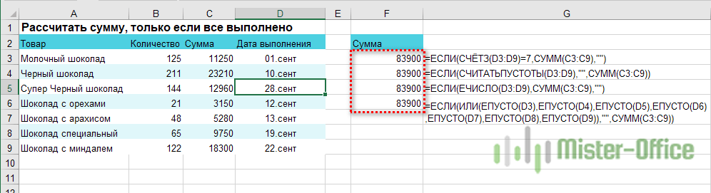
Чтобы выполнить действие только тогда, когда ячейка не пуста (содержит какие-то значения), вы можете использовать формулу Excel, основанную на функции ЕСЛИ.

В примере ниже столбец F содержит даты завершения закупок шоколада.

Поскольку даты для Excel — это числа, то наша задача состоит в том, чтобы проверить в ячейке наличие числа.

Формула в ячейке F3:

=ЕСЛИ(СЧЁТЗ(D3:D9)=7;СУММ(C3:C9);»»)

Как работает эта формула?

Функция СЧЕТЗ (английский вариант — COUNTA) подсчитывает количество значений (текстовых, числовых и логических) в диапазоне ячеек Excel. Если мы знаем количество значений в диапазоне, то легко можно составить условие. Если число значений равно числу ячеек Excel, то значит, пустых среди них нет и можно производить вычисление. Если такого равенства нет, значит есть хотя бы одна пустая ячейка, и вычислять нельзя.

Согласитесь, что нельзя назвать этот способ определения наличия пустых ячеек удобным. Ведь число строк в таблице может измениться, и нужно будет менять формулу: вместо цифры 7 ставить другое число.

Давайте рассмотрим и другие варианты. В ячейке F6 записана большая формула, которая должна проверить условие «если не пусто».

=ЕСЛИ(ИЛИ(ЕПУСТО(D3);ЕПУСТО(D4);ЕПУСТО(D5);ЕПУСТО(D6);
ЕПУСТО(D7);ЕПУСТО(D8);ЕПУСТО(D9));»»;СУММ(C3:C9))

Функция ЕПУСТО (английский вариант — ISBLANK) проверяет, не ссылается ли она на пустую ячейку. Если это так, то возвращает ИСТИНА.

Функция ИЛИ (английский вариант — OR) позволяет объединить условия и указать, что нам достаточно того, чтобы хотя бы одна функция ЕПУСТО обнаружила пустую ячейку. В этом случае никаких вычислений не производим и функция ЕСЛИ возвращает пустую строку. А вот если не пусто – то производим вычисления.

Все достаточно просто, но перечислять кучу ссылок на ячейки не слишком удобно. К тому же, здесь, как и в предыдущем случае, формула не масштабируема: при изменении таблицы она нуждается в корректировке. Это не слишком удобно, да и забыть можно сделать это.

Рассмотрим теперь более универсальные решения.

=ЕСЛИ(СЧИТАТЬПУСТОТЫ(D3:D9);»»;СУММ(C3:C9))

В качестве аргумента условия в функции ЕСЛИ мы используем СЧИТАТЬПУСТОТЫ (английский вариант — COUNTBLANK). Она возвращает количество пустых ячеек, но любое число больше 0 Excel интерпретирует как ИСТИНА.

И, наконец, еще одна формула ЕСЛИ (IF) в Excel, которая проверит «если не пусто» и позволит производить расчет только при наличии непустых ячеек.

=ЕСЛИ(ЕЧИСЛО(D3:D9);СУММ(C3:C9);»»)

Функция ЕЧИСЛО (или ISNUMBER) возвращает ИСТИНА, если ссылается на число. Естественно, при ссылке на пустую ячейку возвратит ЛОЖЬ.

А теперь посмотрим, как это работает. Заполним таблицу недостающим значением.

Как видите, все наши формулы рассчитаны и возвратили одинаковые значения.

А теперь рассмотрим как проверить, что ячейки не пустые, если в них могут быть записаны не только числа, но и текст.

Итак, перед нами уже знакомое выражение

=ЕСЛИ(СЧЁТЗ(D3:D9)=7;СУММ(C3:C9);»»)

Для функции СЧЕТЗ не имеет значения, число или текст используются в ячейке Excel.

=ЕСЛИ(СЧИТАТЬПУСТОТЫ(D3:D9);»»;СУММ(C3:C9))

То же можно сказать и о функции СЧИТАТЬПУСТОТЫ.

А вот третий вариант — к проверке условия при помощи функции ЕЧИСЛО добавляем проверку ЕТЕКСТ (ISTEXT в английском варианте). Объединяем их функцией ИЛИ.

=ЕСЛИ(ИЛИ(ЕТЕКСТ(D3:D9);ЕЧИСЛО(D3:D9));СУММ(C3:C9);»»)

А теперь вставляем в ячейку D5 недостающее значение и проверяем, все ли работает.

Итак, мы с вами убедились, что простая на первый взгляд функция Excel ЕСЛИ дает нам на самом деле много возможностей для операций с данными.

Надеемся, этот материал был полезен. А вот еще несколько примеров работы с условиями «если – то» при помощи функции ЕСЛИ (IF) в Excel.

Примеры использования функции ЕСЛИ:

Функция ЕСЛИОШИБКА – примеры формул — В статье описано, как использовать функцию ЕСЛИОШИБКА в Excel для обнаружения ошибок и замены их пустой ячейкой, другим значением или определённым сообщением. Покажем примеры, как использовать функцию ЕСЛИОШИБКА с функциями визуального…

Сравнение ячеек в Excel — Вы узнаете, как сравнивать значения в ячейках Excel на предмет точного совпадения или без учета регистра. Мы предложим вам несколько формул для сопоставления двух ячеек по их значениям, длине или количеству…

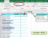проверка правильности ввода Excel при помощи функции ЕСЛИ

Как проверить правильность ввода данных в Excel? — Подтверждаем правильность ввода галочкой. Задача: При ручном вводе данных в ячейки таблицы проверять правильность ввода в соответствии с имеющимся списком допустимых значений. В случае правильного ввода в отдельном столбце ставить…

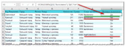Функция ЕСЛИ: проверяем условия с текстом — Рассмотрим использование функции ЕСЛИ в Excel в том случае, если в ячейке находится текст. СодержаниеПроверяем условие для полного совпадения текста.ЕСЛИ + СОВПАДИспользование функции ЕСЛИ с частичным совпадением текста.ЕСЛИ + ПОИСКЕСЛИ…

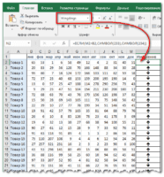Визуализация данных при помощи функции ЕСЛИ — Функцию ЕСЛИ можно использовать для вставки в таблицу символов, которые наглядно показывают происходящие с данными изменения. К примеру, мы хотим показать в отдельной колонке таблицы, происходит рост или снижение продаж.…

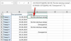3 примера, как функция ЕСЛИ работает с датами. — На первый взгляд может показаться, что функцию ЕСЛИ для работы с датами можно применять так же, как для числовых и текстовых значений, которые мы только что обсудили. К сожалению, это…

Источник

This Excel tutorial explains how to use the Excel IF function with syntax and examples.

Description

The Microsoft Excel IF function returns one value if the condition is TRUE, or another value if the condition is FALSE.

The IF function is a built-in function in Excel that is categorized as a Logical Function. It can be used as a worksheet function (WS) in Excel. As a worksheet function, the IF function can be entered as part of a formula in a cell of a worksheet.

If you want to follow along with this tutorial, download the example spreadsheet.

Download Example

Syntax

The syntax for the IF function in Microsoft Excel is:

IF( condition, value_if_true, [value_if_false] )

Parameters or Arguments

condition: The value that you want to test.
value_if_true: It is the value that is returned if condition evaluates to TRUE.
value_if_false: Optional. It is the value that is returned if condition evaluates to FALSE.

Returns

The IF function returns value_if_true when the condition is TRUE.
The IF function returns value_if_false when the condition is FALSE.
The IF function returns FALSE if the value_if_false parameter is omitted and the condition is FALSE.

Example (as Worksheet Function)

Let’s explore how to use the IF function as a worksheet function in Microsoft Excel.

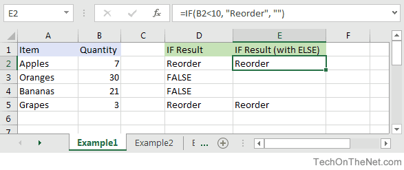
Based on the Excel spreadsheet above, the following IF examples would return:

=IF(B2<10, "Reorder", "")
Result: "Reorder"

=IF(A2="Apples", "Equal", "Not Equal")
Result: "Equal"

=IF(B3>=20, 12, 0)
Result: 12

Combining the IF function with Other Logical Functions

Quite often, you will need to specify more complex conditions when writing your formula in Excel. You can combine the IF function with other logical functions such as AND, OR, etc. Let’s explore this further.

AND function

The IF function can be combined with the AND function to allow you to test for multiple conditions. When using the AND function, all conditions within the AND function must be TRUE for the condition to be met. This comes in very handy in Excel formulas.

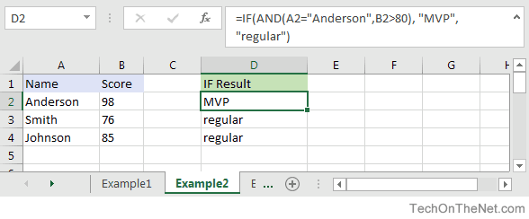
Based on the spreadsheet above, you can combine the IF function with the AND function as follows:

=IF(AND(A2="Anderson",B2>80), "MVP", "regular")
Result: "MVP"

=IF(AND(B2>=80,B2<=100), "Great Score", "Not Bad")
Result: "Great Score"

=IF(AND(B3>=80,B3<=100), "Great Score", "Not Bad")
Result: "Not Bad"

=IF(AND(A2="Anderson",A3="Smith",A4="Johnson"), 100, 50)
Result: 100

=IF(AND(A2="Anderson",A3="Smith",A4="Parker"), 100, 50)
Result: 50

In the examples above, all conditions within the AND function must be TRUE for the condition to be met.

OR function

The IF function can be combined with the OR function to allow you to test for multiple conditions. But in this case, only one or more of the conditions within the OR function needs to be TRUE for the condition to be met.

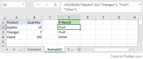
Based on the spreadsheet above, you can combine the IF function with the OR function as follows:

=IF(OR(A2="Apples",A2="Oranges"), "Fruit", "Other")
Result: "Fruit"

=IF(OR(A4="Apples",A4="Oranges"),"Fruit","Other")
Result: "Other"

=IF(OR(A4="Bananas",B4>=100), 999, "N/A")
Result: 999

=IF(OR(A2="Apples",A3="Apples",A4="Apples"), "Fruit", "Other")
Result: "Fruit"

In the examples above, only one of the conditions within the OR function must be TRUE for the condition to be met.

Let’s take a look at one more example that involves ranges of percentages.

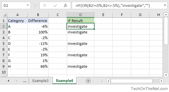
Based on the spreadsheet above, we would have the following formula in cell D2:

=IF(OR(B2>=5%,B2<=-5%),"investigate","")
Result: "investigate"

This IF function would return «investigate» if the value in cell B2 was either below -5% or above 5%. Since -6% is below -5%, it will return «investigate» as the result. We have copied this formula into cells D3 through D9 to show you the results that would be returned.

For example, in cell D3, we would have the following formula:

=IF(OR(B3>=5%,B3<=-5%),"investigate","")
Result: "investigate"

This formula would also return «investigate» but this time, it is because the value in cell B3 is greater than 5%.

Frequently Asked Questions

Question: In Microsoft Excel, I’d like to use the IF function to create the following logic:

if C11>=620, and C10=»F»or»S», and C4<=$1,000,000, and C4<=$500,000, and C7<=85%, and C8<=90%, and C12<=50, and C14<=2, and C15=»OO», and C16=»N», and C19<=48, and C21=»Y», then reference cell A148 on Sheet2. Otherwise, return an empty string.

Answer: The following formula would accomplish what you are trying to do:

=IF(AND(C11>=620, OR(C10="F",C10="S"), C4<=1000000, C4<=500000, C7<=0.85, C8<=0.9, C12<=50, C14<=2, C15="OO", C16="N", C19<=48, C21="Y"), Sheet2!A148, "")

Question: In Microsoft Excel, I’m trying to use the IF function to return 0 if cell A1 is either < 150,000 or > 250,000. Otherwise, it should return A1.

Answer: You can use the OR function to perform an OR condition in the IF function as follows:

=IF(OR(A1<150000,A1>250000),0,A1)

In this example, the formula will return 0 if cell A1 was either less than 150,000 or greater than 250,000. Otherwise, it will return the value in cell A1.

Question: In Microsoft Excel, I’m trying to use the IF function to return 25 if cell A1 > 100 and cell B1 < 200. Otherwise, it should return 0.

Answer: You can use the AND function to perform an AND condition in the IF function as follows:

=IF(AND(A1>100,B1<200),25,0)

In this example, the formula will return 25 if cell A1 is greater than 100 and cell B1 is less than 200. Otherwise, it will return 0.

Question: In Microsoft Excel, I need to write a formula that works this way:

IF (cell A1) is less than 20, then times it by 1,
IF it is greater than or equal to 20 but less than 50, then times it by 2
IF its is greater than or equal to 50 and less than 100, then times it by 3
And if it is great or equal to than 100, then times it by 4

Answer: You can write a nested IF statement to handle this. For example:

=IF(A1<20, A1*1, IF(A1<50, A1*2, IF(A1<100, A1*3, A1*4)))

Question: In Microsoft Excel, I need a formula in cell C5 that does the following:

IF A1+B1 <= 4, return $20
IF A1+B1 > 4 but <= 9, return $35
IF A1+B1 > 9 but <= 14, return $50
IF A1+B1 >= 15, return $75

Answer: In cell C5, you can write a nested IF statement that uses the AND function as follows:

=IF((A1+B1)<=4,20,IF(AND((A1+B1)>4,(A1+B1)<=9),35,IF(AND((A1+B1)>9,(A1+B1)<=14),50,75)))

Question: In Microsoft Excel, I need a formula that does the following:

IF the value in cell A1 is BLANK, then return «BLANK»
IF the value in cell A1 is TEXT, then return «TEXT»
IF the value in cell A1 is NUMERIC, then return «NUM»

Answer: You can write a nested IF statement that uses the ISBLANK function, the ISTEXT function, and the ISNUMBER function as follows:

=IF(ISBLANK(A1)=TRUE,"BLANK",IF(ISTEXT(A1)=TRUE,"TEXT",IF(ISNUMBER(A1)=TRUE,"NUM","")))

Question: In Microsoft Excel, I want to write a formula for the following logic:

IF R1<0.3 AND R2<0.3 AND R3<0.42 THEN «OK» OTHERWISE «NOT OK»

Answer: You can write an IF statement that uses the AND function as follows:

=IF(AND(R1<0.3,R2<0.3,R3<0.42),"OK","NOT OK")

Question: In Microsoft Excel, I need a formula for the following:

IF cell A1= PRADIP then value will be 100
IF cell A1= PRAVIN then value will be 200
IF cell A1= PARTHA then value will be 300
IF cell A1= PAVAN then value will be 400

Answer: You can write an IF statement as follows:

=IF(A1="PRADIP",100,IF(A1="PRAVIN",200,IF(A1="PARTHA",300,IF(A1="PAVAN",400,""))))

Question: In Microsoft Excel, I want to calculate following using an «if» formula:

if A1<100,000 then A1*.1% but minimum 25
and if A1>1,000,000 then A1*.01% but maximum 5000

Answer: You can write a nested IF statement that uses the MAX function and the MIN function as follows:

=IF(A1<100000,MAX(25,A1*0.1%),IF(A1>1000000,MIN(5000,A1*0.01%),""))

Question: In Microsoft Excel, I am trying to create an IF statement that will repopulate the data from a particular cell if the data from the formula in the current cell equals 0. Below is my attempt at creating an IF statement that would populate the data; however, I was unsuccessful.

=IF(IF(ISERROR(M24+((L24-S24)/AA24)),"0",M24+((L24-S24)/AA24)))=0,L24)

The initial part of the formula calculates the EAC (Estimate At completion = AC+(BAC-EV)/CPI); however if the current EV (Earned Value) is zero, the EAC will equal zero. IF the outcome is zero, I would like the BAC (Budget At Completion), currently recorded in another cell (L24), to be repopulated in the current cell as the EAC.

Answer: You can write an IF statement that uses the OR function and the ISERROR function as follows:

=IF(OR(S24=0,ISERROR(M24+((L24-S24)/AA24))),L24,M24+((L24-S24)/AA24))

Question: I have been looking at your Excel IF, AND and OR sections and found this very helpful, however I cannot find the right way to write a formula to express if C2 is either 1,2,3,4,5,6,7,8,9 and F2 is F and F3 is either D,F,B,L,R,C then give a value of 1 if not then 0. I have tried many formulas but just can’t get it right, can you help please?

Answer: You can write an IF statement that uses the AND function and the OR function as follows:

=IF(AND(C2>=1,C2<=9, F2="F",OR(F3="D",F3="F",F3="B",F3="L",F3="R",F3="C")),1,0)

Question:In Excel, I have a roadspeed of a car in m/s in cell A1 and a drop down menu of different units in C1 (which unclude mph and kmh). I have used the following IF function in B1 to convert the number to the unit selected from the dropdown box:

=IF(C1="mph","=A1*2.23693629",IF(C1="kmh","A1*3.6"))

However say if kmh was selected B1 literally just shows A1*3.6 and does not actually calculate it. Is there away to get it to calculate it instead of just showing the text message?

Answer: You are very close with your formula. Because you are performing mathematical operations (such as A1*2.23693629 and A1*3.6), you do not need to surround the mathematical formulas in quotes. Quotes are necessary when you are evaluating strings, not performing math.

Try the following:

=IF(C1="mph",A1*2.23693629,IF(C1="kmh",A1*3.6))

Question:For an IF statement in Excel, I want to combine text and a value.

For example, I want to put an equation for work hours and pay. IF I am paid more than I should be, I want it to read how many hours I owe my boss. But if I work more than I am paid for, I want it to read what my boss owes me (hours*Pay per Hour).

I tried the following:

=IF(A2<0,"I owe boss" abs(A2) "Hours","Boss owes me" abs(A2)*15 "dollars")

Is it possible or do I have to do it in 2 separate cells? (one for text and one for the value)

Answer: There are two ways that you can concatenate text and values. The first is by using the & character to concatenate:

=IF(A2<0,"I owe boss " & ABS(A2) & " Hours","Boss owes me " & ABS(A2)*15 &  " dollars")

Or the second method is to use the CONCATENATE function:

=IF(A2<0,CONCATENATE("I owe boss ", ABS(A2)," Hours"), CONCATENATE("Boss owes me ", ABS(A2)*15,  " dollars"))

Question:I have Excel 2000. IF cell A2 is greater than or equal to 0 then add to C1. IF cell B2 is greater than or equal to 0 then subtract from C1. IF both A2 and B2 are blank then equals C1. Can you help me with the IF function on this one?

Answer: You can write a nested IF statement that uses the AND function and the ISBLANK function as follows:

=IF(AND(ISBLANK(A2)=FALSE,A2>=0),C1+A2, IF(AND(ISBLANK(B2)=FALSE,B2>=0),C1-B2, IF(AND(ISBLANK(A2)=TRUE, ISBLANK(B2)=TRUE),C1,"")))

Question:How would I write this equation in Excel? IF D12<=0 then D12*L12, IF D12 is > 0 but <=600 then D12*F12, IF D12 is >600 then ((600*F12)+((D12-600)*E12))

Answer: You can write a nested IF statement as follows:

=IF(D12<=0,D12*L12,IF(D12>600,((600*F12)+((D12-600)*E12)),D12*F12))

Question:In Excel, I have this formula currently:

=IF(OR(A1>=40, B1>=40, C1>=40), "20", (A1+B1+C1)-20)

If one of my salesman does sale for $40-$49, then his commission is $20; however if his/her sale is less (for example $35) then the commission is that amount minus $20 ($35-$20=$15). I have 3 columns that are needed based on the type of sale. Only one column per row will be needed. The problem is that, when left blank, the total in the formula cell is -20. I need help setting up this formula so that when the 3 columns are left blank, the cell with the formula is left blank as well.

Answer: Using the AND function and the ISBLANK function, you can write your IF statement as follows:

=IF(AND(ISBLANK(A1),ISBLANK(B1),ISBLANK(C1)),"",IF(OR(A1>40, B1>40, C1>40), "20", (A1+B1+C1)-20))

In this formula, we are using the ISBLANK function to check if all 3 cells A1, B1, and C1 are blank, and if they are return a blank value («»). Then the rest is the formula that you originally wrote.

Question:In Excel, I need to create a simple booking and and out system, that shows a date out and a date back

«A1» = allows person to input date booked out
«A2» =allows person to input date booked back in

«A3″= shows status of product, eg, booked out, overdue return etc.

I can automate A3 with the following IF function:

=IF(ISBLANK(A2),"booked out","returned")

But what I cant get to work is if the product is out for 10 days or more, I would like the cell to say «send email»

Can you assist?

Answer: Using the TODAY function and adding an additional IF function, you can write your formula as follows:

=IF(ISBLANK(A2),IF(TODAY()-A1>10,"send email","booked out"),"returned")

Question:Using Microsoft Excel, I need a formula in cell U2 that does the following:

IF the date in E2<=12/31/2010, return T2*0.75
IF the date in E2>12/31/2010 but <=12/31/2011, return T2*0.5
IF the date in E2>12/31/2011, return T2*0

I tried using the following formula, but it gives me «#VALUE!»

=IF(E2<=DATE(2010,12,31),T2*0.75), IF(AND(E2>DATE(2010,12,31),E2<=DATE(2011,12,31)),T2*0.5,T2*0)

Can someone please help? Thanks.

Answer: You were very close…you just need to adjust your parentheses as follows:

=IF(E2<=DATE(2010,12,31),T2*0.75, IF(AND(E2>DATE(2010,12,31),E2<=DATE(2011,12,31)),T2*0.5,T2*0))

Question:In Excel, I would like to add 60 days if grade is ‘A’, 45 days if grade is ‘B’ and 30 days if grade is ‘C’. It would roughly look something like this, but I’m struggling with commas, brackets, etc.

(IF C5=A)=DATE(YEAR(B5)+0,MONTH(B5)+0,DAY(B5)+60),
(IF C5=B)=DATE(YEAR(B5)+0,MONTH(B5)+0,DAY(B5)+45),
(IF C5=C)=DATE(YEAR(B5)+0,MONTH(B5)+0,DAY(B5)+30)

Answer:You should be able to achieve your date calculations with the following formula:

=IF(C5="A",B5+60,IF(C5="B",B5+45,IF(C5="C",B5+30)))

Question:In Excel, I am trying to write a function and can’t seem to figure it out. Could you help?

IF D3 is < 31, then 1.51
IF D3 is between 31-90, then 3.40
IF D3 is between 91-120, then 4.60
IF D3 is > 121, then 5.44

Answer:You can write your formula as follows:

=IF(D3>121,5.44,IF(D3>=91,4.6,IF(D3>=31,3.4,1.51)))

Question:I would like ask a question regarding the IF statement. How would I write in Excel this problem?

I have to check if cell A1 is empty and if not, check if the value is less than equal to 5. Then multiply the amount entered in cell A1 by .60. The answer will be displayed on Cell A2.

Answer:You can write your formula in cell A2 using the IF function and ISBLANK function as follows:

=IF(AND(ISBLANK(A1)=FALSE,A1<=5),A1*0.6,"")

Question:In Excel, I’m trying to nest an OR command and I can’t find the proper way to write it. I want the spreadsheet to do the following:

If D6 equals «HOUSE» and C6 equals either «MOUSE» or «CAT», I want to return the value in cell B6. Otherwise, the formula should return the value «BLANK».

I tried the following:

=IF((D6="HOUSE")*(C6="MOUSE")*OR(C6="CAT"));B6;"BLANK")

If I only ask for HOUSE and MOUSE or HOUSE and CAT, it works, but as soon as I ask for MOUSE OR CAT, it doesn’t work.

Answer:You can write your formula using the AND function and OR function as follows:

=IF(AND(D6="HOUSE",OR(C6="MOUSE",C6="CAT")),B6,"BLANK")

This will return the value in B6 if D6 equals «HOUSE» and C6 equals either «MOUSE» or «CAT». If those conditions are not met, the formula will return the text value of «BLANK».

Question:In Microsoft Excel, I’m trying to write the following formula:

If cell A1 equals «jaipur», «udaipur» or «jodhpur», then cell A2 should display «rajasthan»
If cell A1 equals «bangalore», «mysore» or «belgum», then cell A2 should display «karnataka»

Please help.

Answer:You can write your formula using the OR function as follows:

=IF(OR(A1="jaipur",A1="udaipur",A1="jodhpur"),"rajasthan", IF(OR(A1="bangalore",A1="mysore",A1="belgum"),"karnataka"))

This will return «rajasthan» if A1 equals either «jaipur», «udaipur» or «jodhpur» and it will return «karnataka» if A1 equals either «bangalore», «mysore» or «belgum».

Question:In Microsoft Excel I’m trying to achieve the following with IF function:

If a value in any cell in column F is «food» then add the value of its corresponding cell in column G (eg a corresponding cell for F3 is G3). The IF function is performed in another cell altogether. I can do it for a single pair of cells but I don’t know how to do it for an entire column. Could you help?

At the moment, I’ve got this:

=IF(F3="food"; G3; 0)

Answer:This formula can be created using the SUMIF formula instead of using the IF function:

=SUMIF(F1:F10,"=food",G1:G10)

This will evaluate the first 10 rows of data in your spreadsheet. You may need to adjust the ranges accordingly.

I notice that you separate your parameters with semi-colons, so you might need to replace the commas in the formula above with semi-colons.

Question:I’m looking for an Exel formula that says:

If F3 is «H» and E3 is «H», return 1
If F3 is «A» and E3 is «A», return 2
If F3 is «d» and E3 is «d», return 3

Appreciate if you can help.

Answer:This Excel formula can be created using the AND formula in combination with the IF function:

=IF(AND(F3="H",E3="H"),1,IF(AND(F3="A",E3="A"),2,IF(AND(F3="d",E3="d"),3,"")))

We’ve defaulted the formula to return a blank if none of the conditions above are met.

Question:I am trying to get Excel to check different boxes and check if there is text/numbers listed in the cells and then spit out «Complete» if all 5 Boxes have text/Numbers or «Not Complete» if one or more is empty. This is what I have so far and it doesn’t work.

=IF(OR(ISBLANK(J2),ISBLANK(M2),ISBLANK(R2),ISBLANK (AA2),ISBLANK (AB2)),"Not Complete","")

Answer:First, you are correct in using the ISBLANK function, however, you have a space between ISBLANK and (AA2), as well as ISBLANK and (AB2). This might seem insignificant, but Excel can be very picky and will return a #NAME? error. So first you need to eliminate those spaces.

Next, you need to change the ELSE condition of your IF function to return «Complete».

You should be able to modify your formula as follows:

=IF(OR(ISBLANK(J2),ISBLANK(M2),ISBLANK(R2),ISBLANK(AA2),ISBLANK(AB2)), "Not Complete", "Complete")

Now if any of the cell J2, M2, R2, AA2, or AB2 are blank, the formula will return «Not Complete». If all 5 cells have a value, the formula will return «Complete».

Question:I’m very new to the Excel world, and I’m trying to figure out how to set up the proper formula for an If/then cell.

What I’m trying for is:

If B2’s value is 1 to 5, then multiply E2 by .77
If B2’s value is 6 to 10, then multiply E2 by .735
If B2’s value is 11 to 19, then multiply E2 by .7
If B2’s value is 20 to 29, then multiply E2 by .675
If B2’s value is 30 to 39, then multiply E2 by .65

I’ve tried a few different things thinking I was on the right track based on the IF, and AND function tutorials here, but I can’t seem to get it right.

Answer:To write your IF formula, you need to nest multiple IF functions together in combination with the AND function.

The following formula should work for what you are trying to do:

=IF(AND(B2>=1, B2<=5), E2*0.77, IF(AND(B2>=6, B2<=10), E2*0.735, IF(AND(B2>=11, B2<=19), E2*0.7, IF(AND(B2>=20, B2<=29), E2*0.675, IF(AND(B2>=30, B2<=39), E2*0.65,"")))))

As one final component of your formula, you need to decide what to do when none of the conditions are met. In this example, we have returned «» when the value in B2 does not meet any of the IF conditions above.

Question:Here is the Excel formula that has me between a rock and a hard place.

If E45 <= 50, return 44.55
If E45 > 50 and E45 < 100, return 42
If E45 >=200, return 39.6

Again thank you very much.

Answer:You should be able to write this Excel formula using a combination of the IF function and the AND function.

The following formula should work:

=IF(E45<=50, 44.55, IF(AND(E45>50, E45<100), 42, IF(E45>=200, 39.6, "")))

Please note that if none of the conditions are met, the Excel formula will return «» as the result.

Question:I have a nesting OR function problem:

My nonworking formula is:

=IF(C9=1,K9/J7,IF(C9=2,K9/J7,IF(C9=3,K9/L7,IF(C9=4,0,K9/N7))))

In Cell C9, I can have an input of 1, 2, 3, 4 or 0. The problem is on how to write the «or» condition when a «4 or 0» exists in Column C. If the «4 or 0» conditions exists in Column C I want Column K divided by Column N and the answer to be placed in Column M and associated row

Answer:You should be able to use the OR function within your IF function to test for C9=4 OR C9=0 as follows:

=IF(C9=1,K9/J7,IF(C9=2,K9/J7,IF(C9=3,K9/L7,IF(OR(C9=4,C9=0),K9/N7))))

This formula will return K9/N7 if cell C9 is either 4 or 0.

Question:In Excel, I am trying to create a formula that will show the following:

If column B = Ross and column C = 8 then in cell AB of that row I want it to show 2013, If column B = Block and column C = 9 then in cell AB of that row I want it to show 2012.

Answer:You can create your Excel formula using nested IF functions with the AND function.

=IF(AND(B1="Ross",C1=8),2013,IF(AND(B1="Block",C1=9),2012,""))

This formula will return 2013 as a numeric value if B1 is «Ross» and C1 is 8, or 2012 as a numeric value if B1 is «Block» and C1 is 9. Otherwise, it will return blank, as denoted by «».

Question:In Excel, I really have a problem looking for the right formula to express the following:

If B1=0, C1 is equal to A1/2
If B1=1, C1 is equal to A1/2 times 20%
If D1=1, C1 is equal to A1/2-5

I’ve been trying to look for any same expressions in your site. Please help me fix this.

Answer:In cell C1, you can use the following Excel formula with 3 nested IF functions:

=IF(B1=0,A1/2, IF(B1=1,(A1/2)*0.2, IF(D1=1,(A1/2)-5,"")))

Please note that if none of the conditions are met, the Excel formula will return «» as the result.

Question:In Excel, I need the answer for an IF THEN statement which compares column A and B and has an «OR condition» for column C. My problem is I want column D to return yes if A1 and B1 are >=3 or C1 is >=1.

Answer:You can create your Excel IF formula as follows:

=IF(OR(AND(A1>=3,B1>=3),C1>=1),"yes","")

Please note that if none of the conditions are met, the Excel formula will return «» as the result.

Question:In Excel, what have I done wrong with this formula?

=IF(OR(ISBLANK(C9),ISBLANK(B9)),"",IF(ISBLANK(C9),D9-TODAY(), "Reactivated"))

I want to make an event that if B9 and C9 is empty, the value would be empty. If only C9 is empty, then the output would be the remaining days left between the two dates, and if the two cells are not empty, the output should be the string ‘Reactivated’.

The problem with this code is that IF(ISBLANK(C9),D9-TODAY() is not working.

Answer:First of all, you might want to replace your OR function with the AND function, so that your Excel IF formula looks like this:

=IF(AND(ISBLANK(C9),ISBLANK(B9)),"",IF(ISBLANK(C9),D9-TODAY(),"Reactivated"))

Next, make sure that you don’t have any abnormal formatting in the cell that contains the results. To be safe, right click on the cell that contains the formula and choose Format Cells from the popup menu. When the Format Cells window appears, select the Number tab. Choose General as the format and click on the OK button.

Question:I was wondering if you could tell me what I am doing wrong.
Here are the instructions:

A customer is eligible for a discount if the customer’s 2016 sales greater than or equal to 100000 OR if the customers First Order was placed in 2016.
If the customer qualifies for a discount, return a value of Y
If the customer does not qualify for a discount, return a value of N.

Here is the formula I’ve entered:

=IF(OR([2014 Sales]=0,[2015 Sales]=0,[2016 Sales]>=100000),"Y","N")

I only have 2 cells wrong. Can you help me please? I am very lost and confused.

Answer:You are very close with your IF formula, however, it looks like you need to add the AND function to your formula as follows:

=IF(OR([2016 Sales]>=100000,AND([2014 Sales]=0,[2015 Sales]=0),C8>=100000),"Y","N")

This formula should return Y if 2016 sales are greater than or equal to 100000, or if both 2014 sales and 2015 sales are 0. Otherwise, the formula will return N. You will also notice that we switched the order of your conditions in the formula so that it is easier to understand the formula based on your instructions above.

Question:Could you please help me? I need to use «OR» on my formula but I can’t get it to work. This is what I’ve tried:

=IF(C6>=0<=150,150000,IF(C6>=151<=160,158400))

Here is what I need the formula to do:

IF C6 IS >=0 OR <=150 THEN ASSIGN $150000

IF C6 IS >=151 OR <=160 THEN ASSIGN $158400

Answer:You should be able to use the AND function within your IF function as follows:

=IF(AND(ISBLANK(C6)=FALSE,C6>=0,C6<=150),150000,IF(AND(C6>=151,C6<=160),158400,""))

Notice that we first use the ISBLANK function to test C6 to make sure that it is not blank. This is because if C6 if blank, it will evalulate to greater than 0 and thus return 150000. To avoid this, we include ISBLANK(C6)=FALSE as one of the conditions in addition to C6>=0 and C6<=150. That way, you won’t return any false results if C6 is blank.

Question:I am having a problem with a formula, I want it to be IF E5=N then do the first formula, else do the second formula. Excel recognizes the =IF(logical_test,value_if_TRUE,value_if_FALSE) but doesn’t like the formula below:

=IF(e5="N",((AND(AH5-AG5<456, AH5-S5<822)), "Compliant", "not Compliant"),((AH5-S5<822), "Compliant", "not Compliant"))

Any help would be greatly appreciated.

Answer:To have the first formula executed when E5=N and then second formula executed when E5<>N, you will need to nest 2 additional IF functions within the main IF function as follows:

=IF(E5="N", IF((AND(AH5-AG5<456, AH5-S5<822)), "Compliant", "not Compliant"), IF((AH5-S5<822), "Compliant", "not Compliant"))

If E5=»N», the first nested IF function will be executed:

IF((AND(AH5-AG5<456, AH5-S5<822)), "Compliant", "not Compliant")

Otherwise,the second nested IF function will be executed:

IF((AH5-S5<822), "Compliant", "not Compliant"))

Question:I need to write a formula based on the following logic:

There is a maximum discount allowed of £1000 if the capital sum is less that £43000 and a lower discount of £500 if the capital sum is above £43000. So the formula should return either £500 or £1000 in the cell but the £43000 is made up of two numbers, say for e.g. £42750+350 and if the second number is less than the allowed discount, the actual lower value is returned — in this case the £500 or £1000 becomes £350. Or as another e.g. £42000+750 returns £750.

So on my spreadsheet, in this second e.g. I would have A1= £42000, A2=750, A3=A1+A2, A4=the formula with the changing discount, in this case £750.

How can I write this formula?

Answer:In cell A4, you can calculate the correct discount using the IF function and the MIN function as follows:

=IF(A3<43000, MIN(A2,1000), MIN(A2,500))

If A3 is less than 43000, the formula will return the lower value of A2 and 1000. Otherwise, it will return the lower value of A2 and 500.

Question: I have a list of sizes in column A with sizes 100, 200, 300, 400, 500, 600. Then I have another column B, with sizes of my products, and it is random, for example, 318, 445, 527. What I’m trying to create is for a value of 318 in column B, I need to return 400 for that product. If the value in column B is 445, then I should return 500 and so on, as long sizes in column A must be BIGGER to the NEAREST size to column B.

Any idea how to create this function?

Answer:If your sizes are in increments of 100, you can create this function by taking the value in column B, dividing by 100, rounding up to the nearest integer, and then multiplying by 100.

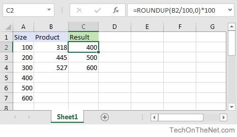
For example in cell C2, you can use the IF function and the ROUNDUP function as follows:

=ROUNDUP(B2/100,0)*100

This will return the correct value of 400 for a value of 318 in cell B2. Just copy this formula to cell C3, C4 and so on.

Источник

Функция ЕСЛИ в Excel — это отличный инструмент для проверки условий на ИСТИНУ или ЛОЖЬ. Если значения ваших расчетов равны заданным параметрам функции как ИСТИНА, то она возвращает одно значение, если ЛОЖЬ, то другое.

Содержание

Что возвращает функция
Синтаксис
Аргументы функции
Дополнительная информация
Функция Если в Excel примеры с несколькими условиями
Пример 1. Проверяем простое числовое условие с помощью функции IF (ЕСЛИ)
Пример 2. Использование вложенной функции IF (ЕСЛИ) для проверки условия выражения
Пример 3. Вычисляем сумму комиссии с продаж с помощью функции IF (ЕСЛИ) в Excel
Пример 4. Используем логические операторы (AND/OR) (И/ИЛИ) в функции IF (ЕСЛИ) в Excel
Пример 5. Преобразуем ошибки в значения “0” с помощью функции IF (ЕСЛИ)

Что возвращает функция

Заданное вами значение при выполнении двух условий ИСТИНА или ЛОЖЬ.

Синтаксис

=IF(logical_test, [value_if_true], [value_if_false]) — английская версия

=ЕСЛИ(лог_выражение; [значение_если_истина]; [значение_если_ложь]) — русская версия

Аргументы функции

logical_test (лог_выражение) — это условие, которое вы хотите протестировать. Этот аргумент функции должен быть логичным и определяемым как ЛОЖЬ или ИСТИНА. Аргументом может быть как статичное значение, так и результат функции, вычисления;
[value_if_true] ([значение_если_истина]) — (не обязательно) — это то значение, которое возвращает функция. Оно будет отображено в случае, если значение которое вы тестируете соответствует условию ИСТИНА;
[value_if_false] ([значение_если_ложь]) — (не обязательно) — это то значение, которое возвращает функция. Оно будет отображено в случае, если условие, которое вы тестируете соответствует условию ЛОЖЬ.

Дополнительная информация

В функции ЕСЛИ может быть протестировано 64 условий за один раз;
Если какой-либо из аргументов функции является массивом — оценивается каждый элемент массива;
Если вы не укажете условие аргумента FALSE (ЛОЖЬ) value_if_false (значение_если_ложь) в функции, т.е. после аргумента value_if_true (значение_если_истина) есть только запятая (точка с запятой), функция вернет значение “0”, если результат вычисления функции будет равен FALSE (ЛОЖЬ).
На примере ниже, формула =IF(A1> 20,”Разрешить”) или =ЕСЛИ(A1>20;»Разрешить») , где value_if_false (значение_если_ложь) не указано, однако аргумент value_if_true (значение_если_истина) по-прежнему следует через запятую. Функция вернет “0” всякий раз, когда проверяемое условие не будет соответствовать условиям TRUE (ИСТИНА).

|
Если вы не укажете условие аргумента TRUE(ИСТИНА) (value_if_true (значение_если_истина)) в функции, т.е. условие указано только для аргумента value_if_false (значение_если_ложь), то формула вернет значение “0”, если результат вычисления функции будет равен TRUE (ИСТИНА);
На примере ниже формула равна =IF (A1>20;«Отказать») или =ЕСЛИ(A1>20;»Отказать»), где аргумент value_if_true (значение_если_истина) не указан, формула будет возвращать “0” всякий раз, когда условие соответствует TRUE (ИСТИНА).

Функция Если в Excel примеры с несколькими условиями

Пример 1. Проверяем простое числовое условие с помощью функции IF (ЕСЛИ)

При использовании функции ЕСЛИ в Excel, вы можете использовать различные операторы для проверки состояния. Вот список операторов, которые вы можете использовать:

Ниже приведен простой пример использования функции при расчете оценок студентов. Если сумма баллов больше или равна «35», то формула возвращает “Сдал”, иначе возвращается “Не сдал”.

Пример 2. Использование вложенной функции IF (ЕСЛИ) для проверки условия выражения

Функция может принимать до 64 условий одновременно. Несмотря на то, что создавать длинные вложенные функции нецелесообразно, то в редких случаях вы можете создать формулу, которая множество условий последовательно.

В приведенном ниже примере мы проверяем два условия.

Первое условие проверяет, сумму баллов не меньше ли она чем 35 баллов. Если это ИСТИНА, то функция вернет “Не сдал”;
В случае, если первое условие — ЛОЖЬ, и сумма баллов больше 35, то функция проверяет второе условие. В случае если сумма баллов больше или равна 75. Если это правда, то функция возвращает значение “Отлично”, в других случаях функция возвращает “Сдал”.

Пример 3. Вычисляем сумму комиссии с продаж с помощью функции IF (ЕСЛИ) в Excel

Функция позволяет выполнять вычисления с числами. Хороший пример использования — расчет комиссии продаж для торгового представителя.

В приведенном ниже примере, торговый представитель по продажам:

не получает комиссионных, если объем продаж меньше 50 тыс;
получает комиссию в размере 2%, если продажи между 50-100 тыс
получает 4% комиссионных, если объем продаж превышает 100 тыс.

Рассчитать размер комиссионных для торгового агента можно по следующей формуле:

=IF(B2<50,0,IF(B2<100,B2*2%,B2*4%)) — английская версия

=ЕСЛИ(B2<50;0;ЕСЛИ(B2<100;B2*2%;B2*4%)) — русская версия

В формуле, использованной в примере выше, вычисление суммы комиссионных выполняется в самой функции ЕСЛИ. Если объем продаж находится между 50-100K, то формула возвращает B2 * 2%, что составляет 2% комиссии в зависимости от объема продажи.

Больше лайфхаков в нашем Telegram Подписаться

Пример 4. Используем логические операторы (AND/OR) (И/ИЛИ) в функции IF (ЕСЛИ) в Excel

Вы можете использовать логические операторы (AND/OR) (И/ИЛИ) внутри функции для одновременного тестирования нескольких условий.

Например, предположим, что вы должны выбрать студентов для стипендий, основываясь на оценках и посещаемости. В приведенном ниже примере учащийся имеет право на участие только в том случае, если он набрал более 80 баллов и имеет посещаемость более 80%.

Вы можете использовать функцию AND (И) вместе с функцией IF (ЕСЛИ), чтобы сначала проверить, выполняются ли оба эти условия или нет. Если условия соблюдены, функция возвращает “Имеет право”, в противном случае она возвращает “Не имеет право”.

Формула для этого расчета:

=IF(AND(B2>80,C2>80%),”Да”,”Нет”) — английская версия

=ЕСЛИ(И(B2>80;C2>80%);»Да»;»Нет») — русская версия

Пример 5. Преобразуем ошибки в значения “0” с помощью функции IF (ЕСЛИ)

С помощью этой функции вы также можете убирать ячейки содержащие ошибки. Вы можете преобразовать значения ошибок в пробелы или нули или любое другое значение.

Формула для преобразования ошибок в ячейках следующая:

=IF(ISERROR(A1),0,A1) — английская версия

=ЕСЛИ(ЕОШИБКА(A1);0;A1) — русская версия

Формула возвращает “0”, в случае если в ячейке есть ошибка, иначе она возвращает значение ячейки.

ПРИМЕЧАНИЕ. Если вы используете Excel 2007 или версии после него, вы также можете использовать функцию IFERROR для этого.

Точно так же вы можете обрабатывать пустые ячейки. В случае пустых ячеек используйте функцию ISBLANK, на примере ниже:

=IF(ISBLANK(A1),0,A1) — английская версия

=ЕСЛИ(ЕПУСТО(A1);0;A1) — русская версия

Источник

Simple IF examples

Common problems

Need more help?

See Also

Need more help?

The syntax of the function «IF» with one condition

The function IF in Excel with multiple conditions

Enhanced functionality with the help of the operators «AND» and «OR»

How to compare data in two tables

Что делает функция ЕСЛИ?

Синтаксис функции ЕСЛИ

Простейший пример применения.

Как правильно записать условие «если – то» в Excel?

А если один из параметров не заполнен?

Использование функции ЕСЛИ с числами.

Функция ЕСЛИ: примеры с несколькими условиями.

Вложенные условия с математическими выражениями.

Объединяем несколько условий.

Пример 1

Пример 2.

Пример 3.

Производим вычисления по условию.

Description

Syntax

Parameters or Arguments

Returns

Example (as Worksheet Function)

Combining the IF function with Other Logical Functions

AND function

OR function

Frequently Asked Questions

Что возвращает функция

Синтаксис

Аргументы функции

Дополнительная информация

Функция Если в Excel примеры с несколькими условиями

Пример 1. Проверяем простое числовое условие с помощью функции IF (ЕСЛИ)

Пример 2. Использование вложенной функции IF (ЕСЛИ) для проверки условия выражения

Пример 3. Вычисляем сумму комиссии с продаж с помощью функции IF (ЕСЛИ) в Excel

Пример 4. Используем логические операторы (AND/OR) (И/ИЛИ) в функции IF (ЕСЛИ) в Excel

Пример 5. Преобразуем ошибки в значения “0” с помощью функции IF (ЕСЛИ)