
Microsoft Excel
Q1. Some of your data in Column C is displaying as hashtags (#) because the column is too narrow. How can you widen Column C just enough to show all the data?
- Right-click column C, select Format Cells, and then select Best-Fit.
- Right-click column C and select Best-Fit.
- Double-click column C.
- Double-click the vertical boundary between columns C and D.
Q2. Which two functions check for the presence of numerical or nonnumerical characters in cells?
- ISNUMBER and ISTEXT
- ISNUMBER and ISALPHA
- ISVALUE AND ISNUMBER
- ISVALUE and ISTEXT
Q3. If you drag the fill handle (lower-right corner) of cell A2 downward into cells A3, A4, and A5, what contents will appear in those cells?

- Jan, Jan, Jan
- Feb, Mar, blank cell
- Feb, Mar, Apr
- FEB, MAB, APR
Q4. If cell A3 contains the text THE DEATH OF CHIVALRY, what will the function =PROPER(A3) return?
- the death of chivalry
- The death of Chivalry
- THE DEATH OF CHIVALRY
- The Death Of Chivalry
Q5. In the worksheet below, you want to use Data > Subtotal to show a subtotal value per sport. What must you do BEFORE applying the Subtotal function?

- Sort by the data in Column E.
- Format the data in Column D.
- Sort by the data in Column D.
- Format the data in Column E.
Q6. When editing a cell, what do you press to cycle between relative, mixed, and absolute cell references?
- Alt+F4 (Windows) or Option+F4 (Mac)
- Alt+Shift+4 (Windows) or Option+Shift+4 (Mac)
- Ctrl+Shift+4 (Windows) or Command+Shift+4 (Mac)
- the F4 (Windows) or Command+T (Mac)
Q7. You need to add a line chart showing a sales trends over the last 12 months and you have only a little space to work with. How can you convey the required information within a single cell?
- Add an image of the chart to a comment.
- Add a hyperlink to another worksheet that displays a chart when clicked.
- Add an image of the chart to the worksheet.
- Add a sparkline, a graphic that summarizes data visually within a single worksheet cell.
Q8. What is the best way to activate the Excel Help system?
- Right-click anywhere and select Help.
- Press F1 or click the Help tab in the ribbon.
- Press F10.
- all of these answers.
Q9. Which format will display the value 27,500,000 as 27.5?
- ##,###,,
- ###.0,,
- 999.9,,
- ###,###.0,
Q10. When using Goal Seek, you can find a target result by varying _ at most.
- three inputs
- four inputs
- two inputs
- one input
Q11. In the image below, which option(s) can you select so that the appropriate field headers appear in cells A4 and B3 instead of the terms Row Labels and Column Labels, respectively?

- Show in Tabular Form
- Show in Compact Form
- Show in Compact For or Show in Outline Form
- Show in Tabular Form or Show in Outline Form
Q12. Which formula is NOT equivalent to all of the others?
- =A3+A4+A5+A6
- =SUM(A3:A6)
- =SUM(A3,A6)
- =SUM(A3,A4,A5,A6)
Q13. Which custom format will make the cells in column A appear like the corresponding cells in column B?
- MMM-YYYY
- MMMM-YYYY
- MMMM&»-«&YYYY
- M-YYYY
Q14. Which function returns a reference to a cell (or cell range) that is a specified distance from a base cell?
- OFFSET
- VLOOKUP
- INDEX
- MATCH
Q15. You’re working with columns whose width and font-size should not be changed. Yet the columns are too narrow to display all the text in each cell. What tool should you use to solve the problem?
- Sparklines
- Wrap Text
- Fill Handle
- Centered Alignment
Q16. Of the four chart types listed, which works best for summarizing time-based data?
- pie chart
- line chart
- XY scatter chart
- bar chart
Q17. The AutoSum formulas in the range C9:F9 below return unexpected values. Why is this?

- The AutoSum formulas refer to the column to the left of their cells.
- The AutoSum formulas exclude the bottom row of data.
- The AutoSum formulas include the year at the top of each column in the calculation.
The formula bar clearly shows it's the dates (top row) included, along with the total (bottom) row. Thus, the bottom row of data is not excluded. - The AutoSum formulas include their own cells, creating a circular reference.
Q18. The text filter in column A is designed to display only those rows where column A entry has a particular attribute. What is this attribute?

- The second character in the cell is 9.
- The number 9 appears one or more times within the cell.
- The cell is comprised of 9 characters.
- The number 9 appears once and only once within the cell.
Q19. An organization chart, which shows the hierarchy within a company or organization, is available as _ that is included with Excel.
- a 3D model
- SmartArt
- a Treemap chart
- a drawing object
Q20. You want to be able to restrict values allowed in a cell and need to create a drop-down list of values from which users can choose. Which feature should you use?
- Protect Worksheet
- Conditional Formatting
- Allow Users to Edit Ranges
- Data Validation
Q21. To round up a value to the nearest increment of your choice, such as the next five cents, what function should you use?
- ROUNDUP
- MAX
- ROUND
- CEILING
Q22. Which function returns the largest value amongst all values within the range H2:H30?
- =MAX(H2:H30)
- =MAXIMUM(H2:H30)
- =LARGE(H2:H30,29)
- =UPPER(H2:H30,1)
Q23. Which chart type can display two different data series as a different series type within the same chart?

- XY chart
- clustered column
- bubble chart
- combo chart
Q24. In the image below, what does clicking the button indicated by the green arrow do?

- Hides or shows the formula bar.
- Selects all.
- Hides or shows the ribbon.
- Selects objects.
Q25. Which formula returns the value in cell A1 of the worksheet named MySheet?
- =MySheet!A1
- =MySheet_A1
- =MySheet&A1
- =MySheet@A1
Q26. In the worksheet below, you want to copy the formatting of cell A1 into cells B1:D1. Which approach (see arrows) accomplishes this the most efficiently?

- B
- C
- A
- D
Q27. Which formula correctly counts the number of numeric values in both B4:E4 and G4:I4?
- =COUNT(B4:E4&G4:I4)
- =COUNT(B4:E4,G4:I4)
- =COUNT(B4:E4 G4:I4)
- =COUNT(B4:I4)
Q28. After activating a chart, which sequence adds a trendline to the chart?
- In the Format group, select Trendline from the Insert Shapes list.
- Click outside the plot area and select Add Trendline
- Click inside the plot and select Forecast.
- Right-click a data series and select Add Trendline.
Q29. Which Excel add-in will help you find a target result by varying multiple inputs to a formula?
- Goal Seek
- Power Pivot
- Data Analysis
- Solver
Q30. What tool would you use to prevent the input in a cell of a date outside a specific range?
- Protect Workbook
- Watch Window
- Data Validation
- Filter
Q31. When you sort a list of numerical value into ascending or descending order, the value in the middle of the list is the _.
- mode
- modulus
- average
- median
Q32. Which format setting does not change the background appearance of a cell?
- Cell style
- Fill color
- Pattern style
- Font color
Q33. In Excel, what do most formulas begin with?
- :
- =
- (
- —
Q34. You need to determine the commission earned by each Sales Rep, based on the Sales amounts in B3:B50 and the Commission rate specified in cell A1. You want to enter a formula in C3 and copy it down to C50. Which formula should you use?
| A | B | C | |
|---|---|---|---|
| 1 | 8.5% | 2018 Commission | |
| 2 | Sales Rep | 2018 Sales | Commission Earned |
| 3 | Jordan Hinton | $123,938.00 | |
| 4 | Lilah Douglas | $5594,810.00 | |
| 5 | Karyn Reese | $235,954.00 | |
| 6 | Chiquita Walsh | $684,760.00 |
- =$A1*B3
- =$A$1*B3
- =A1*$B3
- =A1*B3
Q35. If you start a date series by dragging down the fill handle of a single cell that contains the date 12/1/19, what will you get?
- a series of consecutive days following the initial date
- a series of days exactly one month apart
- a series of days identical to the initial date
- a series of days exactly one year apart
Q36. To discover how many cells in a range contain values that meet a single criterion, use the _ function.
- COUNT
- SUMIFS
- COUNTA
- COUNTIF
Q37. Your worksheet has the value 27 in cell B3. What value is returned by the function =MOD (B3,6)?
- 4
- 1
- 5
- 3
Q38. For an IF function to check whether cell B3 contains a value between 15 and 20 inclusively, what condition should you use?
- OR(B3=>15,B3<=20)
- AND (B3>=15,B3<=20)
- OR(B3>15,B3<20)
- AND(B3>15, B3<20)
Q39. The charts below are based on the data in cells A3:G5. The chart on the right was created by copying the one on the left. Which ribbon button was clicked to change the layout of the chart on the right?

- Move Chart
- Switch Row/Column
- Quick Layout
- Change Chart Type
Q40. Cell A20 displays an orange background when its value is 5. Changing the value to 6 changes the background color to green. What type of formatting is applied to cell A20?
- Value Formatting
- Cell Style Formatting
- Conditional Formatting
- Tabular format
Q41. What does this formula do? =Sum(Sheet1:Sheet4!D18)
- It adds data from cell D18 of Sheet1 and cell D18 of Sheet4
- It adds data from cell A1 of Sheet1 and cell D18 of sheet4
- It adds all data in the range A1:D18 in Sheet1, Sheet2, Sheet3 and Sheet4
- It adds data from all D18 cells in Sheet1, Sheet2, Sheet3 and Sheet4
Q42. What is the term for an expression that is entered into a worksheet cell and begins with an equal sign?
- function
- argument
- formula
- contents
Q43. How does the appearance of an array formula differ from that of a standard formula?
- In a worksheet cell, array formulas have a small blue triangle in the cell’s upper-right corner.
- A heavy border appears around the range that is occupied by the array formula.
- In the formula bar, an array formula appears surrounded by curly brackets.
- When a cell that contains an array formula is selected, range finders appear on the worksheet around the formula’s precedent cells.
Q44. In a worksheet, column A contains employee last names, column B contains their middle initials (if any), and column C contains their first names. Which tool can combine the last names, initials, and first names in column D without using a worksheet formula?
- Concatenation
- Columns to Text
- Flash Fill
- AutoFill
Q45. Which formula returns the value in cell A10 of the worksheet named Budget Variances?
- =’Budget Variances’!A10
- =’Budget Variances!A10′
- =»BudgetVariances!A10″
- =»BudgetVariances»!A10
Q46. Which function returns the leftmost five characters in cell A1?
- =FIND(A1,1,5)
- =SEARCH(A1,5)
- =LEFT(A1,5)
- =A1-RIGHT(A1,LEN(A1)-5)
Q47. Which function returns TRUE if cell A1 contains a text value?
- =ISALPHA(A1)
- =ISCHAR(A1)
- =ISSTRING(A1)
- =ISTEXT(A1)
Q48. You select cell A1, hover the pointer over the cell border to reveal the move icon, then drag the cell to a new location. Which ribbon commands achieve the same result?
- Cut and Fill
- Cut and Paste
- Copy and Transpose
- Copy and Paste
Q49. You want to add a column to the PivotTable below that shows a 5% bonus for each sales rep. That data does not exists in the original data table. How can you do this without adding more data to the table?

- Add a new PivotTable field.
- Add a calculated item
- Add a new Summarize Value By field.
- Add a calculated field.
Q50. You need to determine the commission earned by each Sales rep, based on the Sales amount in B3:B50 and the Commission rate specified in cell A1. You want to enter a formula in C3 and copy it down to C50. Which formula should you use?

- =A1*$B3
- =A1*B3
- =$A$1*B3
- =$A1*B3
Q51. The NOW() function returns the current date and time as 43740.665218. Which part of this value indicates the time?
- 6652
- 43740.665218
- 43740
- 665218
Q52. Cell A2 contains the value 8 and cell B2 contains the value 9. What happens when cells A2 and B2 are merged and then unmerged?
- Both values are lost.
- Cell A2 contains the value 8 and cell B2 is empty.
- Cell A2 contains the value 8 and cell B2 contains the value 9.
- Cell A2 contains the value 17 and cell B2 is empty.
Q53. In the formula =VLOOKUP(A1,D1:H30,3,FALSE), the lookup value (A1) is being looked for in _.
- column D
- columns D through H
- column H
- column F
Q54. An .xlsx workbook is saved into .csv format. What is preserved in the new .csv file?
- cell values only
- cell values and formats
- cell values and formulas
- cell value, formats, and formulas
Q55. Which function, when entered into cell G7, allows you to determine the sum total of annual sles for market regions 18 and greater?

-
=SUMIF(G2:G6,">17",F2:F6) -
=SUM(G2:G6,">=18,F2:F6) -
=SUMIF(F2:F6,">=18",G2:G6) -
=SUM(F2:F6,"18+",G2:G6)
Q56. Which function, when entered into cell F2 and then dragged to cell F6, returns the performance rating text (e.g., «Good», «Poor») for each representative?

-
=RIGHT(E2,LEN(E2)-27) -
=LEN(E2,MID(E2)-27) -
=LEFT(E2,LEN(E2)-27) -
=RIGHT(E2,MID(E2)-27)
Q57. What is Colors[Inventory] referring to here?
=SUMIFS(Colors[Inventory],Colors[Colors],"Orange")
- the Inventory worksheet in the Colors workbook
- the Inventory column in the Colors table
- the Colors worksheet in the Inventory workbook
- the named range Colors[Inventory], which does not use Format as Table Feature
Table[Column] can be used instead of cell references (C2:C7).
Reference
Q58. Which VLOOKUP function, when entered into cell L2 and then dragged to cell L5, returns the average number of calls for the representative IDs listed in column J?

-
=VLOOKUP(A2,J2:L5,1,FALSE) -
=VLOOKUP(J2,A$2:C$7,1,FALSE) -
=VLOOKUP(J2,A$2:C$7,3,FALSE) -
=VLOOKUP(J2,A2:C7,3,FALSE)
because we are interested in the value of the 3rd column of the table
Q59. Which formula calculates the total value of a single row of cells across a range of columns?
-
=SUBTOTAL(C1:Y15) -
=SUM(15L:15Z) -
=SUM(C15:Y15) -
=SUM(C11:C35)
the sum of columns C to Y for the same row 15
Q60. Which value is returned when you enter =LEN(C3) into cell F3?

- 4
- 5
- 3
- 2
Q61. How can you create the lower table from the top one when the tables are not linked?

- Select
Paste Special > Values. - Select
Paste Special > Transpose. - Use the
TRANSPOSEfunction - Click
Switch Rows & Columns
because it needs to be transposed without creating a reference
Q62. Which function returns the number of characters in a text string in cell A1?
-
=RIGHT(A1)-LEFT(A1)+1 -
=LEN(A1) -
=EXACT(A1) -
=CHARS(A1)
Q63. Which formula, when entered into cell D2 and then dragged to cell D6, calculates the average total number of minutes spent on phone calls for each representative?

-
=B$2*C$2 -
=$C$2/$B$2 -
=C2/B2 -
=B2*C2
Q64. The PivotTable below has one row field and two column fields. How can you pivot this table to show the column fields as subtotals of each value in the row field?

- On the PivotTable itself, drag each
Averagefield into the row fields area. - Right-click a cell in the PivotTable and select
PivotTable Options > Classic PivotTable layout. - In the
PivotTable Fieldspane, dragSum Valuesfrom theColumnssection to a location below the field in theRowssection. - In the
PivotTable Fieldspane, drag each field from theSum Valuessection to theRowssection.
Reference
Q65. Which Excel feature allows you to hide rows or columns with an easily visible expand/collapse?

- grouping
- filtering
- hiding
- cut and paste
Q66. Monthly revenues of 2019 are entered in B2:M2, as shown below, To get year-to-date running total revenues, what formula should you enter in B3 and autofill through M3?

-
=SUMIF($B$2:$M$2,"COLUMN($B$2:$M$2)<=COLUMN())") -
=SUM($B2:B2) -
=SUM(OFFSET($A1,0,0,1,COLUMN())) -
=B2+B3
we are calculating the running total here
Q67. From which field list was the pivotTalble created?
(missing screenshot)
- rows:event, donor / values: Sum of amount
- columns: event / row:donor / values: Sum of amount
- rows:donor, event / values: Sum of amount
- filter: event / row:donor / values: Sum of amount
Q68. In the worksheet shown below, cell C6 contains the formula=VLOOKUP(A6,$F$2:$G$10,2,FALSE). What is the most likely reason that #N/A is returned in cell C6 instead of mallory’s ID (2H54)

- The absolute/relative cell references in the formula are wrong
- Cell A6 is not actualy text its a formula that need to be copied and pasted as a value
- Column C in the lookup range is not sorted properly
- A trailing space probably exist in cell A6 or F7
Q69. What is the difference between pressing the delete key and using the clear command in the Home tab’s Editing group?
- deletes removes the entire column or row. Clear removes the content from the column or row
- deletes removes formulas, values and hyperlinks. clear removes formulas, values, hyperlinks, formats, comments and notes
- Delete removes the cell itself, shifting cells either up or to the left. Clear removes content and properties but does not muves cells
- Delete removes formulas and values. clear removes formulas, values, hyperlinks, formats, comments and notes
Q70. What is the intersection of a worksheet row and column?
- cell
- selection
- element
- scalar
Q71. In this PivotTable, the continuous variable weight is shown in the Row field. Another continuous variable is in the Sum Values field. It is important to reduce a long list of body weights to a smaller set of weight categories. How do you do this?

- Use weight as a filter field as well as a row field in the PivotTable.
- Use
IF()to show weight by categories instead of by pounds. - Click the Row Labels arrow and select Group.
- Right-click any row field value in the PivotTable and select Group.
Q72. How can you drill down into a PivotTable to show details?
- Select the cell into which you want to drill down, right-click, and select Show Summary.
- Select the cell into which you want to drill down, right-click and select Drill-down.
- Select the cell into which you want to drill down and double-click.
- Select the cell into which you want to drill down, right-click and select Show Details > Summary Page
Q73. To ensure the VLOOKUP function returns the value of an exact match, what do you need to enter into the Range_lookup field?

- 0
- 1
- FALSE
- TRUE
Q74. Cell D2 contains the formula =B2-C2. What is the fastest way to copy that formula into cells D3:D501 (the bottom of the data set)?

- Right-click D2 and select Fill Down.
- Click D2’s fill handle and drag it down to D501.
- On the ribbon’s Data tab, select Flash fill.
- Double-click D2’s fill handle.
Q75. This data needs to be sorted by Group, then by Last Name, then by First Name. How do you accomplish this?

- A
- Rearrange the columns in this order: Group, Last Name, First Name.
- Right-click any of the headers.
- Select Sort All.
- B
- Select any cell in the dataset.
- In the Data tab, click the Sort button.
- Add two levels to the default level.
- Populate the Sort-by fields in this order: Group, Last Name, First Name.
- C
- Highlight the entire dataset.
- In the Data tab, click the Sort button. The headers appear.
- Drag the headers into this order: Group, Last Name, First Name.
- D
- Select a cell in the Group column, then sort.
- Select a cell in the Last Name column, then sort.
- Select a cell in the FIrst Name column, then sort.
Q76. How can you use Format Painter to apply the format of a single source cell to several nonadjacent destination cells?
-
A
- Right-click the source cell.
- Click the Format Painter.
- Right-click each destination cell.
- Press Esc.
-
B
- Ctrl-click (Windows) or Command-click (Mac) each destination cell to select it.
- Click the Format Painter.
- Click the source cell.
-
C
- Select the source cell.
- Double-click the Format Painter.
- Click each destination cell.
- Press Esc.
-
D
- Select the source cell.
- Right-click the Format Painter.
- Click each destination cell.
- Press Esc.
Q77. Which is a valid Excel formula?
-
=(A5+B5)*B7 -
=A3-7(B3:B5+4) -
=(A5+B5)B7 -
=B3^[2*/3]
Q78. Columns D, E, and F are hidden in your worksheet. What is one way to unhide these columns?
- Select column G, then right-click and select
Unhide. - Select column C, then right-click and select
Unhide. - On the Page Layout tab, in the
RowsandColumnssection, selectUnhide. - Click and drag to select columns C and G, then right-click and select
Unhide.
Q79. Before publishing a document, you want to identify issues that may make it difficult for people with disabilities to read. Which feature should you use?
- Check Accessibility
- Check Compatibility
- Protect Document
- Inspect Document
Q80. How do you remove the background of an inserted image?
- Select the image and, on the
Picture Tools Formattab, use theCompress Picturefeature. - Select the image and, on the
Designtab, use theFormat Backgroundfeature. - On the
Drawing Tools Formattab, selectGraphics Fill>Remove Background. - Select the image and, on the
Picture Tools Formattab, click the Remove Background button.
Q81. What is the result of the formula =4&3?
- 43
- 12
- #VALUE!
- 7
Q82. How do you remove everything (values, formatting, etc.) from a cell?
- Select the cell. On the Home tab, click Clear.
- Select the cell and press Delete.
- Right-click the cell and select Delete.
- Select the cell. On the Home tab, click Clear > Clear All.
Q83. What is the difference between a workbook and a worksheet?
- An Excel file is a workbook. A workbook contains one or more worksheets.
- Nothing-these two terms mean the same thing.
- A workbook contains only data. A worksheet contains both data and formulas.
- An Excel file is a worksheet. A worksheet contains one or more workbooks.
Q84. How would you connect the slicer to both PivotTables?

- You cannot use one slicer for two PivotTables.
- Right-click the slicer and select Slicer Settings.
- Merge the two PivotTables, right-click the merged PivotTable, and select Combine Slicer.
- Right-click the slicer and select Report Connections, or click Report Connections on the Slicer tab.
https://sfmagazine.com/post-entry/may-2020-excel-sharing-a-pivot-table-slicer-between-multiple-data-sets/
Q85. Which formula contains a valid absolute reference?
-
=B7*$G$3 -
=(B7)*G3 -
=B7*$[G3] -
=B7$*G3
Q86. What happens if you use the AutoSum button in cell H4?

- AutoSum shows the total in the bottom-right of the page
- AutoSum will total the numbers in cells B4:G8
- AutoSum will total the numbers in cells B4:G4
- AutoSum will return a #VALUE! error.
Q87. To create this PivotTable, drag the _ field to the Rows area and the _ field to the Values area?

- Total Sales This Year; Total Sales This Year
- Total Sales This Year; Market Region
- Representative ID Number; Total Sales This Year
- Market Region; Total Sales This Year
Q88. Cell A1 contains the number 3. Which formula returns the text Apple?
-
=SELECT(A1, "Banana", "Orange", "Apple", "Mango") -
=CHOOSE(A1, "Banana", "Orange", "Apple", "Mango") -
=CHOOSE(A1,"Banana","Orange","Apple","Mango") -
=MATCH(A1,{"Banana","Orange","Apple","Mango"})
Q89. Which value is calculated when the formula =AVERAGE(G2:G6)/AVERAGE(C2:C6) is entered into cell H7?

- average number of minutes per call
- average annual sales per minute
- average number sales
- average annual sales per call
Q90. How would you search an entire workbook with Find & Select?
- On the Home tab, click Find & Select > Find > Options (Windows) or Find & Select > Find (Mac). Change the Within drop-down to Workbook.
- On the Home tab, click Find & Select > Find > Options (Windows) or Find & Select > Find (Mac). Change the Look in drop-down to Workbook.
- On the Home tab, click Find & Select > Find > Options (Windows) or Find & Select > Find (Mac). Change the Search drop-down to All.
- You cannot search an entire workbook — you must search the worksheets individually.
Q91. How do you create a heatmap in a table, such as this one, which is responsive to the values?

- map chart
- color scales (within conditional formatting)
- manual highlighting
- data bars (within conditional formatting)
Q92. To split text across cells without using Merge & Center, click Formt Cells. The, on **
Alignment** tab, click**_**.
- Text control > Merge cells
- Horizontal > Center across selection
- Vertical > Center across selection
- Data tab > Text to columns
Q93. In the worksheet below, what do the symbols in rows 4, 6, 7, and 11 indicate?

- The dates are erroneous, such as October 39, 2015.
- The columns aren’t wide enough to show the full date.
- The time are incorrectly formatted as dates.
- The text is incorrectly formatted as dates.
Q94. You are determining % growth by dividing Growth by Sales. Which Excel function would you use to avoid #DIV/0! errors?

- IFERROR
- ROUND
- ISERROR
- DIVIDE
Q95. You have a worksheet in Excel that will print as 10 pages. How can you ensure that the header row is printed at the top of each page?
- Use Print Titles on the Page Layout tab.
- Use Page Setup from the Backstage View.
- Use Freeze Panes on the View tab.
- Format your data as a table; the header prints automatically.
https://support.microsoft.com/en-us/office/print-headings-or-titles-on-every-page-96719bd4-b93e-4237-8f97-d2cabb1b196a
Q96. Which value is returned when you enter this function into cell G2? =IF(SUM(F2:F6)>12,"Too Many Tardy Days","No Tardiness Issue")

- Too Many Tardy Days
- #NUM!
- No Tardiness Issue
- #REF!
0 + 0 + 3 + 6 + 3 = 12. The formula only dislays «Too Many Tardy Days» when it is more than 12.
Q97. What ribbon command on the Home tab can you use to change a cell’s fill color automatically, based on the value of the cell?
- Conditional Formatting
- Format
- Cell Styles
- Fill
Q98. In this worksheet, how are cells A2:D2 related to cell C4?

- Cells A2:D2 are comments relating to the formula in cell C4.
- Cells A2:D2 are the source of an error in the formula in cell C4.
- Cells A2:D2 are precedents of the formula in cell C4.
- Cells A2:D2 are dependents of the formula in cell C4.
Q99. What is the name given to the numbers in or above each bar in a column chart, as shown?

- data table
- data numbers
- data labels
- data values
Q100. Which chart type provides the best visual display of the relationship between two numeric variables?
- radar chart
- box and whisker chart
- XY scatter chart
- combo chart
Q101. To ensure that a collection of shapes are evenly spaced apart from left to right, select the shapes, click Page Layout > Align, and then click _.
- Distribute Horizontally
- Align Center
- Distribute Vertically
- Align Middle
Q102. A file extension of .xlsm indicates what type of workbook?
- macro-enabled workbook
- XML-standard workbook
- Excel 2003 workbook
- workbook where macros are not allowed
Q103. How do you remove only the conditional formatting from a cell and leave all other formatting intact?
- This is not possible-you can remove only all formatting from a cell.
- Select the cell. On the Home tab, click Conditional Formatting > Clear Rules > Clear Rules from Selected Cells.
- Right-click the cell and select Delete Conditional Formatting.
- Right-click the cell and select Remove Conditional Formatting.
Q104. If a range name is used in a formula and the name is deleted, what happens to the formula?
- The formula display a warning but the actual cell address is substituted for the deleted name.
- The formula becomes invalid and displays a #NAME? error.
- The actual cell addresses replace the original range name in the formula.
- The formula becomes invalid and displays a #N/A error
Reference
Q105. You want to restrict the values entered in a cell to a specified set, such as Hop, Skip, Jump. Which type of data validation should you use?
- input range
- list
- custom
- database
reference
Q106. You want to find the second-largest invoice in a column containing all the invoices in a given month. What function would you use?
- NEXT
- MAX
- LARGE
- MATCH
Q107. How can you see the data in column E?

- Close the workbook without saving and reopen it.
- Turn off conditional formatting.
- On the Home tab of the ribbon, select Fit to Column.
- Expand the width of its column.
Q108. In the worksheet below, a table called Projects extends from cell A1 to D10. Cell D1 contains the text Status. Cell E12 contains the formula =Projects[@Status]. What does this formula return?

- #VALUE!
- a blank cell
- #REF!
- 0
Q109. Which Excel feature allows you to select all cells in the column with inconsistent formulas compared to the rest of the column?

- On the Home tab, click Go To > Special > Column differences.
- On the Formulas tab, click Trace precedents.
- On the Formulas tab, click Trace errors.
- On the Formulas tab, click show formulas
Q110. What is one way to center text in a cell?
- Right-click the cell and select Center (Windows) or Center Text (Mac).
- Select the cell and, on the View tab in the Cells section, click Alignment and select Center (Windows) or Center Text (Mac).
- Select the cell and, on the Home tab in the Alignment section, click Center (Windows) or Center Text (Mac).
- Change the width of the cell until the text is centered.
Reference
Q111. Cell D1 contains the value 7.877. You want cell D1 to display this value as 7.9 but keep the original number in calculations. How can you accomplish this?
- Click the Decrease Decimal button once.
- Click the Decrease Decimal button twice.
- Use the ROUND() function.
- In the Cells group on the Home tab, click Format > Format Cells. Then click the Alignment tab and select Right Indent.
Reference
Q112. Given the image below, what happens if you type «P» in cell A6?

- The word «Perez» appears and immediately the active cell moves down.
- The word «Perez» appears and the active cell remains in Edit mode.
- A pop-up list appears with the previous four names.
- The letter «P» appears.
Q113. To insert a new column to the left of a specific column, right-click the header containing the column’s letter and select _.
- Insert Column
- Paste Special
- Insert
- Insert Column Left
Reference
Q114. Your transactions data set contains more than 10,000 rows. Some rows contain the same transaction. How would you remove the rows containing the identical transactions?
- Filter the relevant column, right-click the column head, and select Remove Duplicates.
- This is possible only with Power Query.
- With the data selected, on the Data tab click Remove Duplicates.
- This is possible only using formulas.
Reference
Q115. A colleague shared an excel file with you, and you want to display a worksheet that is hidden in it. How you can do that?
- On the Home tab, click Unhide.
- On the Review tab, click Unhide Sheet.
- On the View tab, click New Window.
- Right-click on any worksheet tab and select Unhide
Reference
Q116. You have a column of dog breeds that are in all capital letters. What function would you use to convert those dog breeds so that only the first letter of each word is capitalized?
- Sentence
- Upper
- Titlecase
- Proper
Q117. In cell C2, how would you limit the user to choosing one of the company’s five regions(East, Central, North, South, West)?

- Use reference tabs to create a drop-down list
- Use a PivotTable slicer to create a drop-down list
- Insert a table in the data to create a drop-down list
- Use data validation to create a drop-down list
Q118. To calculate gross pay, hours are multiplied by the hourly rate. What formula would you put in cell C4 to then able to copy that cell down to the rest of the column

-
=B1*$B$4 -
=$B1*B4 -
=B1*B4 -
=$B$1*B4
Q119. What do blue row numbers indicate?

- The cells are selected/highlighted
- Excel’s options have been changed
- Certain rows in the data set are hidden
- A filter is applied
Reference
Q120. Based on the data in columns D,G,H, and K below, what formula will calculate the average compensation for full-time employees who have a job rating of 5?

-
=AVERAGEIF(D:D,K2,H:H,5,G:G) -
=AVERAGEIF(G:G,D:D,K2,H:H,5) -
=AVERAGEIFS(K2,H:H,5,G:G) -
=AVERAGEIFS(G:G,D:D,K2,H:H,5)
Q121. Which feature enables you to quickly sort and reduce data to a subset?
- data validation
- conditional formatting
- advanced sort
- filters
Q122. You have a formula in cell A1. You want to display that formula in cell B1. What function can you use in cell B1?
- TEXT
- FORMULATEXT
- ISFORMULA
- ISTEXT
Q123. You want to remove the unprintable characters and unnecessary spaces from column A. What formula would you put into cell B2 to copy down to the rest of the column?

-
=ERROR.TYPE(A2) -
=CLEAN(TRIM(A2)) -
=CHOOSE(A2) -
=TRIM(A2)
Q114. What is the output of the formula =(8+2*3)/7?
- 13
- 2
- 11
- 15
Q115. The amount of sales tax on each sale is calculated as the selling price times the quantity sold times the sales tax rate. What formula would you use in celle E4 to then be able ro copy that cell to the rest of the column?
(missing screenshot)
- =C4D4$B$1
- =(C4*D4)*B1
- =C4D4B1
- =C4*D4(*B1)
Q116. Which is not a way to edit a formula in a cell?
- Press F2.
- Select the cell and then click in the formula bar.
- Double-click the cell
- Right-click the cell and select Edit
Q117. What dows this formula do?
- It adds data form all D18 cells in Sheet1, Sheet2, Sheet3, Sheet4
- It adds data from cell D18 of Sheet1 and cell D18 of Sheet4
- It adds alla data in the range A1:D18 in Sheet1,Shee2, Shee3, and Sheet4
- It adds data from cell A1 of Sheet1 and cell D18 of Sheet4
Q118. You realize that you named a table Quraters and you want to correct it to be Quarters. How could you accomplish this ?
- On the Table Design tab (Windows) or Table tab (Mac), rename the table in the Table Name box.
- Copy the table to another worksheet and rename it Quarters.
- Right click in the table and select Rename.
- On the Table Design tab (Windows) or Table tab (Mac), click Name Manager.
Q119. Which function is best used to look up and retrieve data from a specific row in a table?
- HLOOKUP
- MATCH
- VLOOKUP
- ADDRESS
Q120. When you provide alt text for an image, what type of control are you including?
- password protection
- presentation
- layout
- accessibility
Reference
Q121. Which tool provides the easiest way to create and insert an organizational chart into a presentation?
- Charts
- 3D Models
- Shapes
- SmartArt
Reference%2C%20and%20then%20click%20OK.)
Q122. You are creating a slide that shows annual rainfall in different regions of Europe. What chart type would most effectively communicate that relationship?
- line chart
- scatter chart
- pie chart
- map chart
Q123. Column A contains a list of book titles. To ensure that no book title appears more than once, first you select column A. What should you do next?
- Right-click the column head and select Unique
- On the Home ribbon, click Clear > Duplicates
- On the Data ribbon, click Remove Duplicates
- On the Data ribbon, click **Data Validation
Q124. You want to copy only the cells that are displayed here — not the hidden cells — into another worksheet. After selecting the cells in the worksheet, how do you accomplish this?
- On the View tab, select Visible cells only, Paste into the destination worksheet
- On the Home tab, clear the Hidden cells check box. Paste into the destination worksheet
- Copy the cells. Then in the destination worksheet, click Paste special > Paste only visible cells
- On the Home tab, click Find & Select > Go to special > Visible cells only. Paste into the destination worksheet
Q125. You want to define a reusable process to reshape data (removing blank rows, merging columns, etc.). What toold can you use to accomplush this?
- Power Query
- Data Analysis
- Power Pivot
- Data Modeler
Q126. You want to be able restrict values allowed in a cell and need to create a drop-down list of values from which users can choose. Which feature should you use?
- Project Worksheet
- Data validation
- Conditional Formatting
- Allow Users to Edit Ranges
Q127. Which situation will result in a #REF! error?
- The cell referenced in the error message has been deleted
- A nonnumeric agument is used in a function when a numeric value is expected
- A required operator is omitted in a formula
- The formula contains an undefined range
Q128. Which feature allows formatting to be automatically added to new columns and rows?
- AutoFormat
- conditional formatting
- Format as Table
- PivotTable
Q129. What Excel feature can you use to automatically format cells that are greater than a specified value with designated fill and text colors?
- Flash Fill
- Conditional Formatting
- Format as Table
- Theme Colors
Q130. Which formula could not have been entered in cell C5?

- =SUBTOTAL(9, C2:C4)
- =C2+C3+C4
- =SUBTOTAL(C2:C4)
- =SUM(C2:C4)
Q131. The last two digits of the Representative ID Number is the Office ID. Which function, when entered into cell B2 and then dragged to cell B6, returns the Office ID for each representative?

- =TRIM(A2,2)
- =LEFT(A2,2)
- =RIGHT(A2,2)
- =MID(A2,2)
Q132. What is the fastest way to see the data in column E

- Double-click between column headers E and F
- Double-click between column headers F and G
- On the Home tab of the ribbon, select Fit to Column
- Drag to resize the column
Q133. Excel’s default view contains the Quick Access Toolbar and the ribbon. Which can you customize?
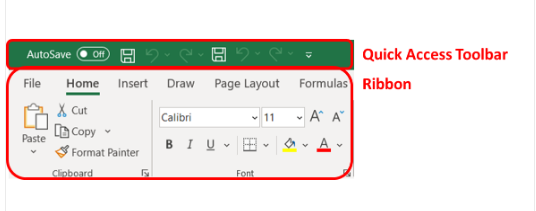
- You cannot customize either.
- only the ribbon
- both the Quick Access Toolbar and the ribbon
- only the Quick Access Toolbar
Q134. Other than pasting an image, how can you insert an image file from your computer into a worksheet?
- On the Insert tab, click Pictures > This Device (Windows) or Pictures > Picture from file (Mac)
- On the Insert tab, click SmartArt > Copy Image from Device (Windows) or SmartArt > Copy (Mac)
- On the Insert tab, click Illustrations > Insert Illustration from This Device
- On the Insert tab, click Icons > Insert > Picture from This Device
Q135. You want to restrict a user from entering any amount greater than $100 or less than $20 in a row. Which Excel feature would you use?
- There is not a feature in Excel that will do this.
- Data Limiting
- Data Parameters
- Data Validation
Q136. What is the output of the formula =(8+2*3)/2?
- 13
- 15
- 11
- 7
Q137. How many columns in Excel sheet by default ?
- 16000
- 1,048,576
- 16384
- 1,048,000
Q138. What feature can you use to populate B2:B7 with the number from each sectence in A2:A7?

- No Excel feature can accomplish this; this is possible only using formulas.
- Flash Fill
- Merge cells
- Text to columns
Q139. Which choice causes a circular error when it is included in a worksheet formula?
- a reference to the cell occupied by the formula
- a named constant
- a worksheet function
- a defined formula name
Q140. You have a workheet with the year in column A, the month in column B, and the day in column C. All fields contain numbers. What function would you use to create the date column in D?
- DATEVALUE
- CONCATENATE
- TEXTJOIN
- DATE
Q141. You have a column containing runner times for a recent race. What function could you use to find the second-place finisher (the runner with the second-lowest time)?
- SMALL
- MATCH
- MIN
- NEXT
Source
Q142. What is the default horizontal alignment of text in a cell
- left
- bottom
- top
- right
Q143. Which formula adds 8 and 5 in a cell?
-
=ADD(8+5) - 8+5
- None of these answers, as you cannot add without a
SUMfunction. -
=8+5
Q144. What feature allow you to make the text appear as it does in cell B1:F1?

- cell border
- merge cells
- text orientation
- wrap text
Q145. What type of chart is this?
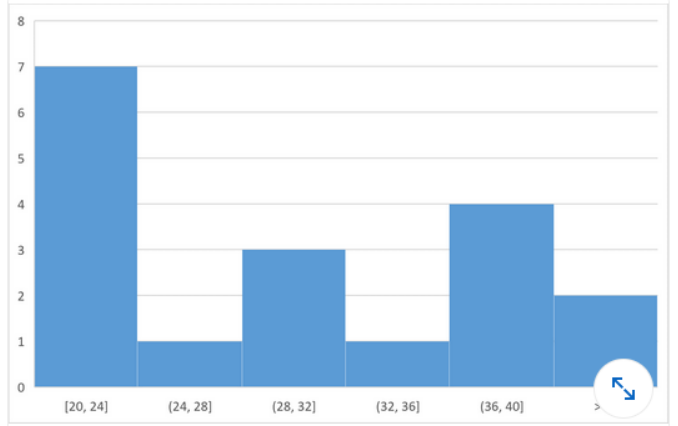
- histogram
- waterfall
- treemap
- box and whisker
Q146. What type of chart is this?

- histogram
- waterfall
- treemap
- box and whisker
In this article, you will find Microsoft Excel LinkedIn Skill Assessment Answer, Use “Ctrl+F” To Find Any Questions or Answers. For Mobile Users, You Just Need To Click On Three dots In Your Browser & You Will Get A “Find” Option There. Use These Options to Get Any Random Questions Answer.
As you already know that this site does not contain only the Linkedin Assessment Answers here, you can also find the solution for other Assessments also. I.e. Fiverr Skills Test answers, Google Course Answers, Coursera Quiz Answers, and Competitive Programming like CodeChef Problems Solutions, & Leetcode Problems Solutions.

100% Free Updated LinkedIn LinkedIn Microsoft Excel Skill Assessment Certification Exam Questions & Answers.
LinkedIn Microsoft Excel Skill Assessment Details:
- 15 – 20 multiple-choice questions
- 1.5 minutes per question
- Score in the top 30% to earn a badge
Before you start:
You must complete this assessment in one session — make sure your internet is reliable.
You can retake this assessment once if you don’t earn a badge.
LinkedIn won’t show your results to anyone without your permission.
After completing the exam, you will get the verified LinkedIn Microsoft Excel Skill Assessment Badge.
LinkedIn Microsoft Excel Skill Assessment Answer
Q1. Some of your data in Column C is displaying as hashtags (#) because the column is too narrow. How can you widen Column C just enough to show all the data?
- Right-click column C, select Format Cells, and then select Best-Fit.
- Right-click column C and select Best-Fit.
- Double-click column C.
- Double-click the vertical boundary between columns C and D.
Q2. Which two functions check for the presence of numerical or nonnumerical characters in cells?
- ISNUMBER and ISTEXT
- ISNUMBER and ISALPHA
- ISVALUE AND ISNUMBER
- ISVALUE and ISTEXT
Q3. If you drag the fill handle (lower-right corner) of cell A2 downward into cells A3, A4, and A5, what contents will appear in those cells?

- Jan, Jan, Jan
- Feb, Mar, blank cell
- Feb, Mar, Apr
- FEB, MAB, APR
Q4. If cell A3 contains the text THE DEATH OF CHIVALRY, what will the function =PROPER(A3) return?
- the death of chivalry
- The death of Chivalry
- THE DEATH OF CHIVALRY
- The Death Of Chivalry
Q5. In the worksheet below, you want to use Data > Subtotal to show a subtotal value per sport. What must you do BEFORE applying the Subtotal function?

- Sort by the data in Column E.
- Format the data in Column D.
- Sort by the data in Column D.
- Format the data in Column E.
Q6. When editing a cell, what do you press to cycle between relative, mixed, and absolute cell references?
- Alt+F4 (Windows) or Option+F4 (Mac)
- Alt+Shift+4 (Windows) or Option+Shift+4 (Mac)
- Ctrl+Shift+4 (Windows) or Command+Shift+4 (Mac)
- the F4 (Windows) or Command+T (Mac)
Q7. You need to add a line chart showing a sales trends over the last 12 months and you have only a little space to work with. How can you convey the required information within a single cell?
- Add an image of the chart to a comment.
- Add a hyperlink to another worksheet that displays a chart when clicked.
- Add an image of the chart to the worksheet.
- Add a sparkline, a graphic that summarizes data visually within a single worksheet cell.
Q8. What is the best way to activate the Excel Help system?
- Right-click anywhere and select Help.
- Press F1 or click the Help tab in the ribbon.
- Press F10.
- all of these answers.
Q9. Which format will display the value 27,500,000 as 27.5?
- ##,###,,
- ###.0,,
- 999.9,,
- ###,###.0,
Q10. When using Goal Seek, you can find a target result by varying _ at most.
- three inputs
- four inputs
- two inputs
- one input
Q11. In the image below, which option(s) can you select so that the appropriate field headers appear in cells A4 and B3 instead of the terms Row Labels and Column Labels, respectively?

- Show in Tabular Form
- Show in Compact Form
- Show in Compact For or Show in Outline Form
- Show in Tabular Form or Show in Outline Form
Q12. Which formula is NOT equivalent to all of the others?
- =A3+A4+A5+A6
- =SUM(A3:A6)
- =SUM(A3,A6)
- =SUM(A3,A4,A5,A6)
Q13. Which custom format will make the cells in column A appear like the corresponding cells in column B?
- MMM-YYYY
- MMMM-YYYY
- MMMM&”-“&YYYY
- M-YYYY
Q14. Which function returns a reference to a cell (or cell range) that is a specified distance from a base cell?
- OFFSET
- VLOOKUP
- INDEX
- MATCH
Q15. You’re working with columns whose width and font-size should not be changed. Yet the columns are too narrow to display all the text in each cell. What tool should you use to solve the problem?
- Sparklines
- Wrap Text
- Fill Handle
- Centered Alignment
Q16. Of the four chart types listed, which works best for summarizing time-based data?
- pie chart
- line chart
- XY scatter chart
- bar chart
Q17. The AutoSum formulas in the range C9:F9 below return unexpected values. Why is this?

- The AutoSum formulas refer to the column to the left of their cells.
- The AutoSum formulas exclude the bottom row of data.
- =The AutoSum formulas include the year at the top of each column in the calculation.
The formula bar clearly shows it's the dates (top row) included, along with the total (bottom) row. Thus, the bottom row of data is not excluded. - The AutoSum formulas include their own cells, creating a circular reference.
Q18. The text filter in column A is designed to display only those rows where column A entry has a particular attribute. What is this attribute?

- The second character in the cell is 9.
- The number 9 appears one or more times within the cell.
- The cell is comprised of 9 characters.
- The number 9 appears once and only once within the cell.
Q19. An organization chart, which shows the hierarchy within a company or organization, is available as _ that is included with Excel.
- a 3D model
- SmartArt
- a Treemap chart
- a drawing object
Q20. You want to be able to restrict values allowed in a cell and need to create a drop-down list of values from which users can choose. Which feature should you use?
- Protect Worksheet
- Conditional Formatting
- Allow Users to Edit Ranges
- Data Validation
Q21. To round up a value to the nearest increment of your choice, such as the next five cents, what function should you use?
- ROUNDUP
- MAX
- ROUND
- CEILING
Q22. Which function returns the largest value amongst all values within the range H2:H30?
- =MAX(H2:H30)
- =MAXIMUM(H2:H30)
- =LARGE(H2:H30,29)
- =UPPER(H2:H30,1)
Q23. Which chart type can display two different data series as a different series type within the same chart?
- XY chart
- clustered column
- bubble chart
- combo chart
Q24. In the image below, what does clicking the button indicated by the green arrow do?

- Hides or shows the formula bar.
- Selects all.
- Hides or shows the ribbon.
- Selects objects.
Q25. Which formula returns the value in cell A1 of the worksheet named MySheet?
- =MySheet!A1
- =MySheet_A1
- =MySheet&A1
- [email protected]
Q26. In the worksheet below, you want to copy the formatting of cell A1 into cells B1:D1. Which approach (see arrows) accomplishes this the most efficiently?

- B
- C
- A
- D
Q27. Which formula correctly counts the number of numeric values in both B4:E4 and G4:I4?
- =COUNT(B4:E4&G4:I4)
- =COUNT(B4:E4,G4:I4)
- =COUNT(B4:E4 G4:I4)
- =COUNT(B4:I4)
Q28. After activating a chart, which sequence adds a trendline to the chart?
- In the Format group, select Trendline from the Insert Shapes list.
- Click outside the plot area and select Add Trendline
- Click inside the plot and select Forecast.
- Right-click a data series and select Add Trendline.
Q29. Which Excel add-in will help you find a target result by varying multiple inputs to a formula?
- Goal Seek
- Power Pivot
- Data Analysis
- Solver
Q30. What tool would you use to prevent the input in a cell of a date outside a specific range?
- Protect Workbook
- Watch Window
- Data Validation
- Filter
Q31. When you sort a list of numerical value into ascending or descending order, the value in the middle of the list is the _.
- mode
- modulus
- average
- median
Q32. Which format setting does not change the background appearance of a cell?
- Cell style
- Fill color
- Pattern style
- Font color
Q33. In Excel, what do most formulas begin with?
- :
- =
- (
- –
Q34. You need to determine the commission earned by each Sales Rep, based on the Sales amounts in B3:B50 and the Commission rate specified in cell A1. You want to enter a formula in C3 and copy it down to C50. Which formula should you use?
| A | B | C | |
|---|---|---|---|
| 1 | 8.5% | 2018 Commission | |
| 2 | Sales Rep | 2018 Sales | Commission Earned |
| 3 | Jordan Hinton | $123,938.00 | |
| 4 | Lilah Douglas | $5594,810.00 | |
| 5 | Karyn Reese | $235,954.00 | |
| 6 | Chiquita Walsh | $684,760.00 |
- =$A1*B3
- =$A$1*B3
- =A1*$B3
- =A1*B3
Q35. If you start a date series by dragging down the fill handle of a single cell that contains the date 12/1/19, what will you get?
- a series of consecutive days following the initial date
- a series of days exactly one month apart
- a series of days identical to the initial date
- a series of days exactly one year apart
Q36. To discover how many cells in a range contain values that meet a single criterion, use the _ function.
- COUNT
- SUMIFS
- COUNTA
- COUNTIF
Q37. Your worksheet has the value 27 in cell B3. What value is returned by the function =MOD (B3,6)?
- 4
- 1
- 5
- 3
Q38. For an IF function to check whether cell B3 contains a value between 15 and 20 inclusively, what condition should you use?
- OR(B3=>15,B3<=20)
- AND (B3>=15,B3<=20)
- OR(B3>15,B3<20)
- AND(B3>15, B3<20)
Q39. The charts below are based on the data in cells A3:G5. The chart on the right was created by copying the one on the left. Which ribbon button was clicked to change the layout of the chart on the right?

- Move Chart
- Switch Row/Column
- Quick Layout
- Change Chart Type
Q40. Cell A20 displays an orange background when its value is 5. Changing the value to 6 changes the background color to green. What type of formatting is applied to cell A20?
- Value Formatting
- Cell Style Formatting
- Conditional Formatting
- Tabular format
Q41. What does this formula do? =Sum(Sheet1:Sheet4!D18)
- It adds data from cell D18 of Sheet1 and cell D18 of Sheet4
- It adds data from cell A1 of Sheet1 and cell D18 of sheet4
- It adds all data in the range A1:D18 in Sheet1, Sheet2, Sheet3 and Sheet4
- It adds data from all D18 cells in Sheet1, Sheet2, Sheet3 and Sheet4
Q42. What is the term for an expression that is entered into a worksheet cell and begins with an equal sign?
- function
- argument
- formula
- contents
Q43. How does the appearance of an array formula differ from that of a standard formula?
- In a worksheet cell, array formulas have a small blue triangle in the cell’s upper-right corner.
- A heavy border appears around the range that is occupied by the array formula.
- In the formula bar, an array formula appears surrounded by curly brackets.
- When a cell that contains an array formula is selected, range finders appear on the worksheet around the formula’s precedent cells.
Q44. In a worksheet, column A contains employee last names, column B contains their middle initials (if any), and column C contains their first names. Which tool can combine the last names, initials, and first names in column D without using a worksheet formula?
- Concatenation
- Columns to Text
- Flash Fill
- AutoFill
Q45. Which formula returns the value in cell A10 of the worksheet named Budget Variances?
- =’Budget Variances’!A10
- =’Budget Variances!A10′
- =”BudgetVariances!A10″
- =”BudgetVariances”!A10
Q46. Which function returns the leftmost five characters in cell A1?
- =FIND(A1,1,5)
- =SEARCH(A1,5)
- =LEFT(A1,5)
- =A1-RIGHT(A1,LEN(A1)-5)
Q47. Which function returns TRUE if cell A1 contains a text value?
- =ISALPHA(A1)
- =ISCHAR(A1)
- =ISSTRING(A1)
- =ISTEXT(A1)
Q48. You select cell A1, hover the pointer over the cell border to reveal the move icon, then drag the cell to a new location. Which ribbon commands achieve the same result?
- Cut and Fill
- Cut and Paste
- Copy and Transpose
- Copy and Paste
Q49. You want to add a column to the PivotTable below that shows a 5% bonus for each sales rep. That data does not exists in the original data table. How can you do this without adding more data to the table?

- Add a new PivotTable field.
- Add a calculated item
- Add a new Summarize Value By field.
- Add a calculated field.
Q50. You need to determine the commission earned by each Sales rep, based on the Sales amount in B3:B50 and the Commission rate specified in cell A1. You want to enter a formula in C3 and copy it down to C50. Which formula should you use?

- =A1*$B3
- =A1*B3
- =$A$1*B3
- =$A1*B3
Q51. The NOW() function returns the current date and time as 43740.665218. Which part of this value indicates the time?
- 6652
- 43740.665218
- 43740
- 665218
Q52. Cell A2 contains the value 8 and cell B2 contains the value 9. What happens when cells A2 and B2 are merged and then unmerged?
- Both values are lost.
- Cell A2 contains the value 8 and cell B2 is empty.
- Cell A2 contains the value 8 and cell B2 contains the value 9.
- Cell A2 contains the value 17 and cell B2 is empty.
Q53. In the formula =VLOOKUP(A1,D1:H30,3,FALSE), the lookup value (A1) is being looked for in _.
- column D
- columns D through H
- column H
- column F
Q54. An .xlsx workbook is saved into .csv format. What is preserved in the new .csv file?
- cell values only
- cell values and formats
- cell values and formulas
- cell value, formats, and formulas
Q55. Which function, when entered into cell G7, allows you to determine the sum total of annual sles for market regions 18 and greater?

-
=SUMIF(G2:G6,">17",F2:F6) -
=SUM(G2:G6,">=18,F2:F6) -
=SUMIF(F2:F6,">=18",G2:G6) -
=SUM(F2:F6,"18+",G2:G6)
Q56. Which function, when entered into cell F2 and then dragged to cell F6, returns the performance rating text (e.g., “Good”, “Poor”) for each representative?

-
=RIGHT(E2,LEN(E2)-27) -
=LEN(E2,MID(E2)-27) -
=LEFT(E2,LEN(E2)-27) -
=RIGHT(E2,MID(E2)-27)
Q57. What is Colors[Inventory] referring to here?
=SUMIFS(Colors[Inventory],Colors[Colors],"Orange")
- the Inventory worksheet in the Colors workbook
- the Inventory column in the Colors table
- the Colors worksheet in the Inventory workbook
- the named range Colors[Inventory], which does not use Format as Table Feature
Table[Column] can be used instead of cell references (C2:C7). Reference
Q58. Which VLOOKUP function, when entered into cell L2 and then dragged to cell L5, returns the average number of calls for the representative IDs listed in column J?

-
=VLOOKUP(A2,J2:L5,1,FALSE) -
=VLOOKUP(J2,A$2:C$7,1,FALSE) -
=VLOOKUP(J2,A$2:C$7,3,FALSE) -
=VLOOKUP(J2,A2:C7,3,FALSE)
because we are interested in the value of the 3rd column of the table
Q59. Which formula calculates the total value of a single row of cells across a range of columns?
-
=SUBTOTAL(C1:Y15) -
=SUM(15L:15Z) -
=SUM(C15:Y15) -
=SUM(C11:C35)
the sum of columns C to Y for the same row 15
Q60. Which value is returned when you enter =LEN(C3) into cell F3?

- 4
- 5
- 3
- 2
Q61. How can you create the lower table from the top one when the tables are not linked?

- Select
Paste Special > Values. - Select
Paste Special > Transpose. - Use the
TRANSPOSEfunction - Click
Switch Rows & Columns
because it needs to be transposed without creating a reference
Q62. Which function returns the number of characters in a text string in cell A1?
-
=RIGHT(A1)-LEFT(A1)+1 -
=LEN(A1) -
=EXACT(A1) -
=CHARS(A1)
Q63. Which formula, when entered into cell D2 and then dragged to cell D6, calculates the average total number of minutes spent on phone calls for each representative?

-
=B$2*C$2 -
=$C$2/$B$2 -
=C2/B2 -
=B2*C2
Q64. The PivotTable below has one row field and two column fields. How can you pivot this table to show the column fields as subtotals of each value in the row field?

- On the PivotTable itself, drag each
Averagefield into the row fields area. - Right-click a cell in the PivotTable and select
PivotTable Options > Classic PivotTable layout. - In the
PivotTable Fieldspane, dragSum Valuesfrom theColumnssection to a location below the field in theRowssection. - In the
PivotTable Fieldspane, drag each field from theSum Valuessection to theRowssection.
Reference
Q65. Which Excel feature allows you to hide rows or columns with an easily visible expand/collapse?

- grouping
- filtering
- hiding
- cut and paste
Q66. Monthly revenues of 2019 are entered in B2:M2, as shown below, To get year-to-date running total revenues, what formula should you enter in B3 and autofill through M3?

-
=SUMIF($B$2:$M$2,"COLUMN($B$2:$M$2)<=COLUMN())") -
=SUM($B2:B2) -
=SUM(OFFSET($A1,0,0,1,COLUMN())) -
=B2+B3
we are calculating the running total here
Q67. From which field list was the pivotTalble created?
(missing screenshot)
- rows:event, donor / values: Sum of amount
- columns: event / row:donor / values: Sum of amount
- rows:donor, event / values: Sum of amount
- filter: event / row:donor / values: Sum of amount
Q68. In the worksheet shown below, cell C6 contains the formula=VLOOKUP(A6,$F$2:$G$10,2,FALSE). What is the most likely reason that #N/A is returned in cell C6 instead of mallory’s ID (2H54)

- The absolute/relative cell references in the formula are wrong
- Cell A6 is not actualy text its a formula that need to be copied and pasted as a value
- Column C in the lookup range is not sorted properly
- A trailing space probably exist in cell A6 or F7
Q69. What is the difference between pressing the delete key and using the clear command in the Home tab’s Editing group?
- deletes removes the entire column or row. Clear removes the content from the column or row
- deletes removes formulas, values and hyperlinks. clear removes formulas, values, hyperlinks, formats, comments and notes
- Delete removes the cell itself, shifting cells either up or to the left. Clear removes content and properties but does not muves cells
- Delete removes formulas and values. clear removes formulas, values, hyperlinks, formats, comments and notes
Q70. What is the intersection of a worksheet row and column?
- cell
- selection
- element
- scalar
Q71. In this PivotTable, the continuous variable weight is shown in the Row field. Another continuous variable is in the Sum Values field. It is important to reduce a long list of body weights to a smaller set of weight categories. How do you do this?

- Use weight as a filter field as well as a row field in the PivotTable.
- Use
IF()to show weight by categories instead of by pounds. - Click the Row Labels arrow and select Group.
- Right-click any row field value in the PivotTable and select Group.
Q72. How can you drill down into a PivotTable to show details?
- Select the cell into which you want to drill down, right-click, and select Show Summary.
- Select the cell into which you want to drill down, right-click and select Drill-down.
- Select the cell into which you want to drill down and double-click.
- Select the cell into which you want to drill down, right-click and select Show Details > Summary Page
Q73. To ensure the VLOOKUP function returns the value of an exact match, what do you need to enter into the Range_lookup field?

- 0
- 1
- FALSE
- TRUE
Q74. Cell D2 contains the formula =B2-C2. What is the fastest way to copy that formula into cells D3:D501 (the bottom of the data set)?

- Right-click D2 and select Fill Down.
- Click D2’s fill handle and drag it down to D501.
- On the ribbon’s Data tab, select Flash fill.
- Double-click D2’s fill handle.
Q75. This data needs to be sorted by Group, then by Last Name, then by First Name. How do you accomplish this?

- A
- Rearrange the columns in this order: Group, Last Name, First Name.
- Right-click any of the headers.
- Select Sort All.
- B
- Select any cell in the dataset.
- In the Data tab, click the Sort button.
- Add two levels to the default level.
- Populate the Sort-by fields in this order: Group, Last Name, First Name.
- C
- Highlight the entire dataset.
- In the Data tab, click the Sort button. The headers appear.
- Drag the headers into this order: Group, Last Name, First Name.
- D
- Select a cell in the Group column, then sort.
- Select a cell in the Last Name column, then sort.
- Select a cell in the FIrst Name column, then sort.
Q76. How can you use Format Painter to apply the format of a single source cell to several nonadjacent destination cells?
- A
- Right-click the source cell.
- Click the Format Painter.
- Right-click each destination cell.
- Press Esc.
- B
- Ctrl-click (Windows) or Command-click (Mac) each destination cell to select it.
- Click the Format Painter.
- Click the source cell.
- C
- Select the source cell.
- Double-click the Format Painter.
- Click each destination cell.
- Press Esc.
- D
- Select the source cell.
- Right-click the Format Painter.
- Click each destination cell.
- Press Esc.
Q77. Which is a valid Excel formula?
-
=(A5+B5)*B7 -
=A3-7(B3:B5+4) -
=(A5+B5)B7 -
=B3^[2*/3]
Q78. Columns D, E, and F are hidden in your worksheet. What is one way to unhide these columns?
- Select column G, then right-click and select
Unhide. - Select column C, then right-click and select
Unhide. - On the Page Layout tab, in the
RowsandColumnssection, selectUnhide. - Click and drag to select columns C and G, then right-click and select
Unhide.
Q79. Before publishing a document, you want to identify issues that may make it difficult for people with disabilities to read. Which feature should you use?
- Check Accessibility
- Check Compatibility
- Protect Document
- Inspect Document
Q80. How do you remove the background of an inserted image?
- Select the image and, on the
Picture Tools Formattab, use theCompress Picturefeature. - Select the image and, on the
Designtab, use theFormat Backgroundfeature. - On the
Drawing Tools Formattab, selectGraphics Fill>Remove Background. - Select the image and, on the
Picture Tools Formattab, click the Remove Background button.
Q81. What is the result of the formula =4&3?
- 43
- 12
- #VALUE!
- 7
Q82. How do you remove everything (values, formatting, etc.) from a cell?
- Select the cell. On the Home tab, click Clear.
- Select the cell and press Delete.
- Right-click the cell and select Delete.
- Select the cell. On the Home tab, click Clear > Clear All.
Q83. What is the difference between a workbook and a worksheet?
- An Excel file is a workbook. A workbook contains one or more worksheets.
- Nothing-these two terms mean the same thing.
- A workbook contains only data. A worksheet contains both data and formulas.
- An Excel file is a worksheet. A worksheet contains one or more workbooks.
Q84. How would you connect the slicer to both PivotTables?

- You cannot use one slicer for two PivotTables.
- Right-click the slicer and select Slicer Settings.
- Merge the two PivotTables, right-click the merged PivotTable, and select Combine Slicer.
- Right-click the slicer and select Report Connections, or click Report Connections on the Slicer tab.
Q85. Which formula contains a valid absolute reference?
-
=B7*$G$3 -
=(B7)*G3 -
=B7*$[G3] -
=B7$*G3
Q86. What happens if you use the AutoSum button in cell H4?

- AutoSum shows the total in the bottom-right of the page
- AutoSum will total the numbers in cells B4:G8
- AutoSum will total the numbers in cells B4:G4
- AutoSum will return a #VALUE! error.
Q87. To create this PivotTable, drag the _ field to the Rows area and the _ field to the Values area?

- Total Sales This Year; Total Sales This Year
- Total Sales This Year; Market Region
- Representative ID Number; Total Sales This Year
- Market Region; Total Sales This Year
Q88. Cell A1 contains the number 3. Which formula returns the text Apple?
-
=SELECT(A1, "Banana", "Orange", "Apple", "Mango") -
=CHOOSE(A1, "Banana", "Orange", "Apple", "Mango") -
=CHOOSE(A1,"Banana","Orange","Apple","Mango") -
=MATCH(A1,{"Banana","Orange","Apple","Mango"})
Q89. Which value is calculated when the formula =AVERAGE(G2:G6)/AVERAGE(C2:C6) is entered into cell H7?

- average number of minutes per call
- average annual sales per minute
- average number sales
- average annual sales per call
Q90. How would you search an entire workbook with Find & Select?
- On the Home tab, click Find & Select > Find > Options (Windows) or Find & Select > Find (Mac). Change the Within drop-down to Workbook.
- On the Home tab, click Find & Select > Find > Options (Windows) or Find & Select > Find (Mac). Change the Look in drop-down to Workbook.
- On the Home tab, click Find & Select > Find > Options (Windows) or Find & Select > Find (Mac). Change the Search drop-down to All.
- You cannot search an entire workbook – you must search the worksheets individually.
Q91. How do you create a heatmap in a table, such as this one, which is responsive to the values?

- map chart
- color scales (within conditional formatting)
- manual highlighting
- data bars (within conditional formatting)
Q92. To split text across cells without using Merge & Center, click Formt Cells. The, on **
Alignment** tab, click**_**.
- Text control > Merge cells
- Horizontal > Center across selection
- Vertical > Center across selection
- Data tab > Text to columns
Q93. In the worksheet below, what do the symbols in rows 4, 6, 7, and 11 indicate?

- The dates are erroneous, such as October 39, 2015.
- The columns aren’t wide enough to show the full date.
- The time are incorrectly formatted as dates.
- The text is incorrectly formatted as dates.
Q94. You are determining % growth by dividing Growth by Sales. Which Excel function would you use to avoid #DIV/0! errors?

- IFERROR
- ROUND
- ISERROR
- DIVIDE
- Use Print Titles on the Page Layout tab.
- Use Page Setup from the Backstage View.
- Use Freeze Panes on the View tab.
- Format your data as a table; the header prints automatically.
Q96. Which value is returned when you enter this function into cell G2? =IF(SUM(F2:F6)>12,"Too Many Tardy Days","No Tardiness Issue")

- Too Many Tardy Days
- #NUM!
- No Tardiness Issue
- #REF!
0 + 0 + 3 + 6 + 3 = 12. The formula only dislays “Too Many Tardy Days” when it is more than 12.
Q97. What ribbon command on the Home tab can you use to change a cell’s fill color automatically, based on the value of the cell?
- Conditional Formatting
- Format
- Cell Styles
- Fill

- Cells A2:D2 are comments relating to the formula in cell C4.
- Cells A2:D2 are the source of an error in the formula in cell C4.
- Cells A2:D2 are precedents of the formula in cell C4.
- Cells A2:D2 are dependents of the formula in cell C4.
Q99. What is the name given to the numbers in or above each bar in a column chart, as shown?

- data table
- data numbers
- data labels
- data values
Q100. Which chart type provides the best visual display of the relationship between two numeric variables?
- radar chart
- box and whisker chart
- XY scatter chart
- combo chart
Q101. To ensure that a collection of shapes are evenly spaced apart from left to right, select the shapes, click Page Layout > Align, and then click _.
- Distribute Horizontally
- Align Center
- Distribute Vertically
- Align Middle
Q102. A file extension of .xlsm indicates what type of workbook?
- macro-enabled workbook
- XML-standard workbook
- Excel 2003 workbook
- workbook where macros are not allowed
Q103. How do you remove only the conditional formatting from a cell and leave all other formatting intact?
- This is not possible-you can remove only all formatting from a cell.
- Select the cell. On the Home tab, click Conditional Formatting > Clear Rules > Clear Rules from Selected Cells.
- Right-click the cell and select Delete Conditional Formatting.
- Right-click the cell and select Remove Conditional Formatting.
Q104. If a range name is used in a formula and the name is deleted, what happens to the formula?
- The formula display a warning but the actual cell address is substituted for the deleted name.
- The formula becomes invalid and displays a #NAME? error.
- The actual cell addresses replace the original range name in the formula.
- The formula becomes invalid and displays a #N/A error
Reference
Q105. You want to restrict the values entered in a cell to a specified set, such as Hop, Skip, Jump. Which type of data validation should you use?
- input range
- list
- custom
- database
reference
Q106. You want to find the second-largest invoice in a column containing all the invoices in a given month. What function would you use?
- NEXT
- MAX
- LARGE
- MATCH
Q107. How can you see the data in column E?

- Close the workbook without saving and reopen it.
- Turn off conditional formatting.
- On the Home tab of the ribbon, select Fit to Column.
- Expand the width of its column.
Q108. In the worksheet below, a table called Projects extends from cell A1 to D10. Cell D1 contains the text Status. Cell E12 contains the formula =Projects[@Status]. What does this formula return?

- #VALUE!
- a blank cell
- #REF!
- 0
Q109. Which Excel feature allows you to select all cells in the column with inconsistent formulas compared to the rest of the column?

- On the Home tab, click Go To > Special > Column differences.
- On the Formulas tab, click Trace precedents.
- On the Formulas tab, click Trace errors.
- On the Formulas tab, click show formulas
Q110. What is one way to center text in a cell?
- Right-click the cell and select Center (Windows) or Center Text (Mac).
- Select the cell and, on the View tab in the Cells section, click Alignment and select Center (Windows) or Center Text (Mac).
- Select the cell and, on the Home tab in the Alignment section, click Center (Windows) or Center Text (Mac).
- Change the width of the cell until the text is centered.
Reference
Q111. Cell D1 contains the value 7.877. You want cell D1 to display the value as 7.9 but keep the original number in calculations. How can you accomplish this?
- Click the Decrease Decimal button once.
- Click the Decrease Decimal button twice.
- Use the ROUND() function.
- In the Cells group on the Home tab, click Format > Format Cells. Then click the Alignment tab and select Right Indent.
Reference
Q112. Given the image below, what happens if you type “P” in cell A6?

- The word “Perez” appears and immediately the active cell moves down.
- The word “Perez” appears and the active cell remains in Edit mode.
- A pop-up list appears with the previous four names.
- The letter “P” appears.
Q113. To insert a new column to the left of a specific column, right-click the header containing the column’s letter and select _.
- Insert Column
- Paste Special
- Insert
- Insert Column Left
Reference
Q114. Your transactions data set contains more than 10,000 rows. Some rows contain the same transaction. How would you remove the rows containing the identical transactions?
- Filter the relevant column, right-click the column head, and select Remove Duplicates.
- This is possible only with Power Query.
- With the data selected, on the Data tab click Remove Duplicates.
- This is possible only using formulas.
Reference
Q115. A colleague shared an excel file with you, and you want to display a worksheet that is hidden in it. How you can do that?
- On the Home tab, click Unhide.
- On the Review tab, click Unhide Sheet.
- On the View tab, click New Window.
- Right-click on any worksheet tab and select Unhide
Reference
Q116. You have a column of dog breeds that are in all capital letters. What function would you use to convert those dog breeds so that only the first letter of each word is capitalized?
- Sentence
- Upper
- Titlecase
- Proper
Q117. In cell C2, how would you limit the user to choosing one of the company’s five regions(East, Central, North, South, West)?

- Use reference tabs to create a drop-down list
- Use a PivotTable slicer to create a drop-down list
- Insert a table in the data to create a drop-down list
- Use data validation to create a drop-down list
Q118. To calculate gross pay, hours are multiplied by the hourly rate. What formula would you put in cell C4 to then able to copy that cell down to the rest of the column

-
=B1*$B$4 -
=$B1*B4 -
=B1*B4 -
=$B$1*B4
Q119. What do blue row numbers indicate?

- The cells are selected/highlighted
- Excel’s options have been changed
- Certain rows in the data set are hidden
- A filter is applied
Reference
Q120. Based on the data in columns D,G,H, and K below, what formula will calculate the average compensation for full-time employees who have a job rating of 5?

-
=AVERAGEIF(D:D,K2,H:H,5,G:G) -
=AVERAGEIF(G:G,D:D,K2,H:H,5) -
=AVERAGEIFS(K2,H:H,5,G:G) -
=AVERAGEIFS(G:G,D:D,K2,H:H,5)
Q121. Which feature enables you to quickly sort and reduce data to a subset?
- data validation
- conditional formatting
- advanced sort
- filters
Q122. You have a formula in cell A1. You want to display that formula in cell B1. What function can you use in cell B1?
- TEXT
- FORMULATEXT
- ISFORMULA
- ISTEXT
Q123. You want to remove the unprintable characters and unnecessary spaces from column A. What formula would you put into cell B2 to copy down to the rest of the column?

-
=ERROR.TYPE(A2) -
=CLEAN(TRIM(A2)) -
=CHOOSE(A2) -
=TRIM(A2)
Q114. What is the output of the formula =(8+2*3)/7?
- 13
- 7
- 11
- 15
Q115. The amount of sales tax on each sale is calculated as the selling price times the quantity sold times the sales tax rate. What formula would you use in celle E4 to then be able ro copy that cell to the rest of the column?
(missing screenshot)
- =C4D4$B$1
- =(C4*D4)*B1
- =C4D4B1
- =C4*D4(*B1)
Q116. Which is not a way to edit a formula in a cell?
- Press F2.
- Select the cell and then click in the formula bar.
- Double-click the cell
- Right-click the cell and select Edit
Q117. What dows this formula do?
=SUM(Sheet1:Sheet4!D18)
- It adds data form all D18 cells in Sheet1, Sheet2, Sheet3, Sheet4
- It adds data from cell D18 of Sheet1 and cell D18 of Sheet4
- It adds alla data in the range A1:D18 in Sheet1,Shee2, Shee3, and Sheet4
- It adds data from cell A1 of Sheet1 and cell D18 of Sheet4
Q118. You realize that you named a table Quraters and you want to correct it to be Quarters. How could you accomplish this ?
- On the Table Design tab (Windows) or Table tab (Mac), rename the table in the Table Name box.
- Copy the table to another worksheet and rename it Quarters.
- Right click in the table and select Rename.
- On the Table Design tab (Windows) or Table tab (Mac), click Name Manager.
Q119. Which function is best used to look up and retrieve data from a specific row in a table?
- HLOOKUP
- MATCH
- VLOOKUP
- ADDRESS
Q120. When you provide alt text for an image, what type of control are you including?
- password protection
- presentation
- layout
- accessibility
Reference
Q121. Which tool provides the easiest way to create and insert an organizational chart into a presentation?
- Charts
- 3D Models
- Shapes
- SmartArt
Reference%2C%20and%20then%20click%20OK.)
Q122. You are creating a slide that shows annual rainfall in different regions of Europe. What chart type would most effectively communicate that relationship?
- line chart
- scatter chart
- pie chart
- map chart
Q123. Column A contains a list of book titles. To ensure that no book title appears more than once, first you select column A. What should you do next?
- Right-click the column head and select Unique
- On the Home ribbon, click Clear > Duplicates
- On the Data ribbon, click Remove Duplicates
- On the Data ribbon, click **Data Validation
Q124. You want to copy only the cells that are displayed here – not the hidden cells – into another worksheet. After selecting the cells in the worksheet, how do you accomplish this?
- On the View tab, select Visible cells only, Paste into the destination worksheet
- On the Home tab, clear the Hidden cells check box. Paste into the destination worksheet
- Copy the cells. Then in the destination worksheet, click Paste special > Paste only visible cells
- On the Home tab, click Find & Select > Go to special > Visible cells only. Paste into the destination worksheet
Q125. You want to define a reusable process to reshape data (removing blank rows, merging columns, etc.). What toold can you use to accomplush this?
- Power Query
- Data Analysis
- Power Pivot
- Data Modeler
Q126. You want to be able restrict values allowed in a cell and need to create a drop-down list of values from which users can choose. Which feature should you use?
- Project Worksheet
- Data validation
- Conditional Formatting
- Allow Users to Edit Ranges
Q127. Which situation will result in a #REF! error?
- The cell referenced in the error message has been deleted
- A nonnumeric agument is used in a function when a numeric value is expected
- A required operator is omitted in a formula
- The formula contains an undefined range
Q128. Which feature allows formatting to be automatically added to new columns and rows?
- AutoFormat
- conditional formatting
- Format as Table
- PivotTable
Q129. What Excel feature can you use to automatically format cells that are greater than a specified value with designated fill and text colors?
- Flash Fill
- Conditional Formatting
- Format as Table
- Theme Colors
Q130. Which formula could not have been entered in cell C5?

- =SUBTOTAL(9, C2:C4)
- =C2+C3+C4
- =SUBTOTAL(C2:C4)
- =SUM(C2:C4)
Q131. The last two digits of the Representative ID Number is the Office ID. Which function, when entered into cell B2 and then dragged to cell B6, returns the Office ID for each representative?

- =TRIM(A2,2)
- =LEFT(A2,2)
- =RIGHT(A2,2)
- =MID(A2,2)
Disclaimer: Hopefully, this article will be useful for you to find all the LinkedIn Microsoft Excel Skill Assessment answer and grab some premium knowledge with less effort. If this article really helped you in any way then make sure to share it with your friends on social media and let them also know about this amazing Skill Assessment Test. the solution is provided by Chase2learn. This tutorial is only for Educational and Learning purpose.
Please share our posts on social media platforms and also suggest to your friends to Join Our Groups. Don’t forget to subscribe.
FAQs
What is Linkedin Assessment?
The LinkedIn Skill Assessments feature allows you to demonstrate your knowledge of the skills you’ve added to your profile by completing assessments specific to those skills. LinkedIn skills evaluations are a means to demonstrate the skills of job hunters. This is how LinkedIn Skill Assessments can be used.
Is this Skill Assessment Test is free?
Yes, LinkedIn Microsoft Excel Skill Assessment Answer is totally free on LinkedIn for you. The only thing is needed i.e. your dedication toward learning.
When I will get Skill Badge?
Yes, if will Pass the Skill Assessment Test, then you will earn a skill badge that will reflect in your LinkedIn profile. For passing in LinkedIn Skill Assessment, you must score 70% or higher, then only you will get your to skill badge.
How to participate in skill quiz assessment?
It’s good practice to update and tweak your LinkedIn profile every few months. After all, life is dynamic and (I hope) you’re always learning new skills. You will notice a button under the Skills & Endorsements tab within your LinkedIn Profile: ‘Take skill quiz.‘ Upon clicking, you will choose your desired skill test quiz and complete your assessment.
LinkedIn Skill Assessments are a series of multiple-choice exams that allow you to prove the skills that are stated in your profile.
How to get Linkedin Skill Badge?
For getting Linkedin Badge in your profile, you need to score at least 70% and above for getting recognition of skill badges.
If you “grade in the 70th percentile or above”—according to LinkedIn—you officially pass and get a LinkedIn skill badge. The social media site will display your badge on your profile.
How long is Skill Assessment valid for?
Skills assessments that do not specify an expiry date are valid for 3 years from the date of the assessment. If more than 3 years have passed by the time the visa application is made, the skills assessment will no longer be valid.
What is the Benefit of Linkedin Skill Assessment?
- Chances of getting hired will be increased.
- You will earn Linkedin Skill Badge.
- Your Linkedin Profile will rank on top.
- You have a chance to get jobs earlier.
- This Skill Assessment will enhance your technical skills, helps you to get recognized by top recruiters, and advanced your knowledge by testing your mind.
Who can give this Linkedin Skill Assessment Test?
Any Linkedin User, Any engineer, developer, or programmer, who wants to improve their Programming Skills
Anyone interested in improving their whiteboard coding skills
Anyone who wants to become a Software Engineer, SDE, Data Scientist, Machine Learning Engineer, etc.
Any students in college who want to start a career in Data Science
Students who have at least high school knowledge in math and who want to start learning data structures
Any self-taught programmer who missed out on a computer science degree.
How to do LinkedIn skill assessment
The LinkedIn Skill Assessments feature allows you to demonstrate your knowledge of the skills you’ve added on your profile by completing assessments specific to those skills.
A typical assessment consists of 15 multiple choice questions and each question tests at least one concept or subskill. The questions are timed and must be completed in one session. You can view the full list of available Skill Assessments and sample questions for each.
Available Skill Assessments on LinkedIn
.NET Framework, Agile Methodologies, Amazon Web Services (AWS), Android, AngularJS, Angular, AutoCAD, AWS, Bash, C, C#, C++, CSS, GIT, Hadoop, HTML, Java, JavaScript, jQuery, JSON, Maven, and MS Vision, QuickBooks, Revit, etc.
What You Need to Know About LinkedIn Skill Assessments
During a job search, wouldn’t it be great to have a way to prove your proficiency in a specific skill to hiring managers?
Well, now there is. On September 17, LinkedIn launched its new Skill Assessments feature. These are online assessments you can take to demonstrate your proficiency in an area such as MS Excel or jQuery. All assessments have been designed by subject matter and LinkedIn Learning experts, and they’re based on an in-depth content creation and review process. Moreover, these assessments seem to be well received: Research shows that job seekers who’ve completed LinkedIn Skill Assessments are approximately 30 percent more likely to get hired than those who haven’t.
How LinkedIn Skill Assessments work
To take an assessment, all you have to do is navigate to the skills section of your profile and select the relevant Skill Assessment. Note that the test is timed. If you have a disability, you can activate the accessibility for the Skill Assessment feature. This will allow you additional time to complete each question.
Your score is private by default, meaning that you can control the visibility of the results. If you score in the 70th percentile or higher, you’ll pass the assessment and have the option of displaying a “verified skill” badge on your profile. If you don’t pass, you can take the assessment again once you’ve brushed up your skills. However, keep in mind that you can only take each assessment once per three months.
When you’ve completed an assessment, LinkedIn provides you with an outline of your results. In addition, for a limited time, it offers relevant LinkedIn Learning courses for free so you can improve further. You’ll also receive relevant job recommendations.
According to Andrew Martins in his Business News Daily article “LinkedIn Users Can Now Showcase Skill Assessments,” the following assessments are currently available:
Adobe Acrobat, Angular, AWS, Bash, C, C#, C++, CSS, GIT, Hadoop, HTML, Java, Javascript, jQuery, JSON, Maven, MongoDB, MS Excel, MS PowerPoint, MS Project, MS SharePoint, MS Visio, Node.js, Objective-C, PHP, Python, QuickBooks, Ruby, Ruby on Rails, Scala, Swift, WordPress, and XML. Experts believe that there are also more, non-technical assessments in the making.
A good way to showcase your skills
LinkedIn Skill Assessments offer a brilliant way for you to showcase your abilities to potential employers while at the same time giving you the opportunity to hone your skills even further. So, take advantage of what’s offered — and use it to maximize your employability!
Sources:
https://blog.linkedin.com/2019/september/17/announcing-skill-assessments-to-help-you-showcase-your-skills
https://www.businessnewsdaily.com/15288-linkedin-skill-assessments.html
https://medium.com/alternative-digital-marketing/linkedin-skill-assessments-are-they-worth-it-735867ebe6ae
The LinkedIn Skill Assessments feature allows you to demonstrate your knowledge of the skills you’ve added on your profile. Job posters on LinkedIn can also add Skill Assessments as part of the job application process. This allows job posters to more efficiently and accurately verify the crucial skills a candidate should have for a role.

The topics in the MS Excel assessment include:
Formulas and Functions
Working with Data
Formatting
User Interface
Charts
Files and Workbooks
Worksheet Layout
Macros
PivotTables
Statistics
Question Format
Multiple Choice
Language
English, French
Table of Content
- 1 LinkedIn Microsoft Excel Skill Assessment Answers
- 1.1 Some of your data in Column C is displaying as hashtags (#) because the column is too narrow. How can you widen Column C just enough to show all the data?
- 1.2 Which two functions check for the presence of numerical or nonnumerical characters in cells?
- 1.3 If you drag the fill handle (lower-right corner) of cell A2 downward into cells A3, A4, and A5, what contents will appear in those cells?
- 1.4 If cell A3 contains the text THE DEATH OF CHIVALRY, what will the function =PROPER(A3) return?
- 1.5 In the worksheet below, you want to use Data > Subtotal to show a subtotal value per sport. What must you do BEFORE applying the Subtotal function?
- 1.6 When editing a cell, what do you press to cycle between relative, mixed, and absolute cell references?
- 1.7 You need to add a line chart showing a sales trends over the last 12 months and you have only a little space to work with. How can you convey the required information within a single cell?
- 1.8 What is the best way to activate the Excel Help system?
- 1.9 Which format will display the value 27,500,000 as 27.5?
- 1.10 When using Goal Seek, you can find a target result by varying _ at most.
- 1.11 In the image below, which option(s) can you select so that the appropriate field headers appear in cells A4 and B3 instead of the terms Row Labels and Column Labels, respectively?
- 1.12 A cell contains the value 7.877 and you want it to display as 7.9. How can you accomplish this?
- 1.13 Which formula is NOT equivalent to all of the others?
- 1.14 Which custom format will make the cells in column A appear like the corresponding cells in column B?
- 1.15 Which function returns a reference to a cell (or cell range) that is a specified distance from a base cell?
- 1.16 You’re working with columns whose width and font-size should not be changed. Yet the columns are too narrow to display all the text in each cell. What tool should you use to solve the problem?
- 1.17 Of the four chart types listed, which works best for summarizing time-based data?
- 1.18 The AutoSum formulas in the range C9:F9 below return unexpected values. Why is this?
- 1.19 The text filter in column A is designed to display only those rows where column A entry has a particular attribute. What is this attribute?
- 1.20 To ensure shapes and other objects are an equal left-to-right distance apart, select the shapes, click Page Layout > Align, and then click _.
- 1.21 An organization chart, which shows the hierarchy within a company or organization, is available as _ that is included with Excel.
- 1.22 You want to be able to restrict values allowed in a cell and need to create a drop-down list of values from which users can choose. Which feature should you use?
- 1.23 To round up a value to the nearest increment of your choice, such as the next five cents, what function should you use?
- 1.24 Which function returns the largest value amongst all values within the range H2:H30?
- 1.25 Which chart type can display two different data series as a different series type within the same chart?
- 1.26 In the image below, what does clicking the button indicated by the green arrow do?
- 1.27 Which formula returns the value in cell A1 of the worksheet named MySheet?
- 1.28 In the worksheet below, you want to copy the formatting of cell A1 into cells B1:D1. Which approach (see arrows) accomplishes this the most efficiently?
- 1.29 Which formula correctly counts the number of numeric values in both B4:E4 and G4:I4?
- 1.30 After activating a chart, which sequence adds a trendline to the chart?
- 1.31 Which Excel add-in will help you find a target result by varying multiple inputs to a formula?
- 1.32 What tool would you use to prevent the input in a cell of a date outside a specific range?
- 1.33 You want to apply subtotals per sport in the data below. What should you do before applying subtotals?
- 1.34 When you sort a list of numerical value into ascending or descending order, the value in the middle of the list is the _.
- 1.35 Which format setting does not change the background appearance of a cell?
- 1.36 In Excel, what do most formulas begin with?
- 1.37 You need to determine the commission earned by each Sales Rep, based on the Sales amounts in B3:B50 and the Commission rate specified in cell A1. You want to enter a formula in C3 and copy it down to C50. Which formula should you use?
- 1.38 If you start a date series by dragging down the fill handle of a single cell that contains the date 12/1/19, what will you get?
- 1.39 To discover how many cells in a range contain values that meet a single criterion, use the _ function.
- 1.40 Your worksheet has the value 27 in cell B3. What value is returned by the function =MOD (B3,6)?
- 1.41 For an IF function to check whether cell B3 contains a value between 15 and 20 inclusively, what condition should you use?
- 1.42 Which format setting does not change the background appearance of a cell?
- 1.43 The charts below are based on the data in cells A3:G5. The chart on the right was created by copying the one on the left. Which ribbon button was clicked to change the layout of the chart on the right?
- 1.44 Cell A20 displays an orange background when its value is 5. Changing the value to 6 changes the background color to green. What type of formatting is applied to cell A20?
- 1.45 What does this formula do? =Sum(Sheet1:Sheet4!D18)
- 1.46 What is the term for an expression that is entered into a worksheet cell and begins with an equal sign?
- 1.47 How does the appearance of an array formula differ from that of a standard formula?
- 1.48 In a worksheet, column A contains employee last names, column B contains their middle initials (if any), and column C contains their first names. Which tool can combine the last names, initials, and first names in column D without using a worksheet formula?
- 1.49 Which formula returns the value in cell A10 of the worksheet named Budget Variances?
- 1.50 Which function returns the leftmost five characters in cell A1?
- 1.51 Which function returns TRUE if cell A1 contains a text value?
- 1.52 Which of these functions returns the largest value among all values within the range H2:H30?
- 1.53 You select cell A1, hover the pointer over the cell border to reveal the move icon, then drag the cell to a new location. Which ribbon commands achieve the same result?
- 1.54 You want to add a column to the PivotTable below that shows a 5% bonus for each sales rep. That data does not exists in the original data table. How can you do this without adding more data to the table?
- 1.55 You need to determine the commission earned by each Sales rep, based on the Sales amount in B3:B50 and the Commission rate specified in cell A1. You want to enter a formula in C3 and copy it down to C50. Which formula should you use?
- 1.56 The NOW() function returns the current date and time as 43740.665218. Which part of this value indicates the time?
- 1.57 Cell A2 contains the value 8 and cell B2 contains the value 9. What happens when cells A2 and B2 are merged and then unmerged?
- 1.58 In the formula =VLOOKUP(A1,D1:H30,3,FALSE), the lookup value (A1) is being looked for in _.
- 1.59 An .xlsx workbook is saved into .csv format. What is preserved in the new .csv file?
- 1.60 Which function, when entered into cell G7, allows you to determine the sum total of annual sles for market regions 18 and greater?
- 1.61 Which function, when entered into cell F2 and then dragged to cell F6, returns the performance rating text (e.g., “Good”, “Poor”) for each representative?
- 1.62 What is Colors[Inventory] referring to here?
- 1.63 Which VLOOKUP function, when entered into cell L2 and then dragged to cell L5, returns the average number of calls for the representative IDs listed in column J?
- 1.64 Which formula calculates the total value of a single row of cells across a range of columns?
- 1.65 Which value is returned when you enter =LEN(C3) into cell F3?
- 1.66 Q66. How can you create the lower table from the top one when the tables are not linked?
- 1.67 Which function returns the number of characters in a text string in cell A1?
- 1.68 Which formula, when entered into cell D2 and then dragged to cell D6, calculates the average total number of minutes spent on phone calls for each representative?
- 1.69 The PivotTable below has one row field and two column fields. How can you pivot this table to show the column fields as subtotals of each value in the row field?
- 1.70 Which Excel feature allows you to hide rows or columns with an easily visible expand/collapse?
- 1.71 Monthly revenues of 2019 are entered in B2:M2, as shown below, To get year-to-date running total revenues, what formula should you enter in B3 and autofill through M3?
- 1.72 If a worksheet has the value 27 in cell B3, what value is returned by the function =MOD(B3,6)?
- 1.73 From which field list was the pivotTalble created?
- 1.74 In the worksheet shown below, cell C6 contains the formula=VLOOKUP(A6,$F$2:$G$10,2,FALSE). What is the most likely reason that #N/A is returned in cell C6 instead of mallory’s ID (2H54)
- 1.75 What is the difference between pressing the delete key and using the clear command in the Home tab’s Editing group?
- 1.76 What is the intersection of a worksheet row and column?
- 1.77 In this PivotTable, the continuous variable weight is shown in the Row field. Another continuous variable is in the Sum Values field. It is important to reduce a long list of body weights to a smaller set of weight categories. How do you do this?
- 1.78 How can you drill down into a PivotTable to show details?
- 1.79 To ensure the VLOOKUP function returns the value of an exact match, what do you need to enter into the Range_lookup field?
- 1.80 Cell D2 contains the formula =B2-C2. What is the fastest way to copy that formula into cells D3:D501 (the bottom of the data set)?
- 1.81 This data needs to be sorted by Group, then by Last Name, then by First Name. How do you accomplish this?
- 1.82 How can you use Format Painter to apply the format of a single source cell to several nonadjacent destination cells?
- 1.83 Which is a valid Excel formula?
- 1.84 Columns D, E, and F are hidden in your worksheet. What is one way to unhide these columns?
- 1.85 Before publishing a document, you want to identify issues that may make it difficult for people with disabilities to read. Which feature should you use?
- 1.86 How do you remove the background of an inserted image?
- 1.87 You want to group your slides based on their content to better organize your presentation. How would you accomplish this?
- 1.88 What is the result of the formula =4&3?
- 1.89 How do you remove everything (values, formatting, etc.) from a cell?
- 1.90 What is Colors[Inventory] referring to here?
- 1.91 What is the difference between a workbook and a worksheet?
- 1.92 How would you connect the slicer to both PivotTables?
- 1.93 Which formula contains a valid absolute reference?
- 1.94 What happens if you use the AutoSum button in cell H4?
- 1.95 To create this PivotTable, drag the _ field to the Rows area and the _ field to the Values area?
- 1.96 Cell A1 contains the number 3. Which formula returns the text Apple?
- 1.97 Which value is calculated when the formula =AVERAGE(G2:G6)/AVERAGE(C2:C6) is entered into cell H7?
- 1.98 How would you search an entire workbook with Find & Select?
- 1.99 How do you create a heatmap in a table, such as this one, which is responsive to the values?
- 1.100 To split text across cells without using Merge & Center, click Formt Cells. Then, on Alignment tab, click _.
- 1.101 In the worksheet below, what do the symbols in rows 4, 6, 7, and 11 indicate?
- 1.102 You are determining % growth by dividing Growth by Sales. Which Excel function would you use to avoid #DIV/0! errors?
- 1.103 You have a worksheet in Excel that will print as 10 pages. How can you ensure that the header row is printed at the top of each page?
- 1.104 Which value is returned when you enter this function into cell G2? =IF(SUM(F2:F6)>12,”Too Many Tardy Days”,”No Tardiness Issue”)
- 1.105 What ribbon command on the Home tab can you use to change a cell’s fill color automatically, based on the value of the cell?
- 1.106 In this worksheet, how are cells A2:D2 related to cell C4?
- 1.107 What is the name given to the numbers in or above each bar in a column chart, as shown?
- 1.108 Which chart type provides the best visual display of the relationship between two numeric variables?
- 1.109 To ensure that a collection of shapes are evenly spaced apart from left to right, select the shapes, click Page Layout > Align, and then click _.
- 1.110 A file extension of .xlsm indicates what type of workbook?
- 1.111 How do you remove only the conditional formatting from a cell and leave all other formatting intact?
- 1.112 If a range name is used in a formula and the name is deleted, what happens to the formula?
- 1.113 You want to restrict the values entered in a cell to a specified set, such as Hop, Skip, Jump. Which type of data validation should you use?
- 1.114 You want to find the second-largest invoice in a column containing all the invoices in a given month. What function would you use?
- 1.115 How can you see the data in column E?
- 1.116 In the worksheet below, a table called Projects extends from cell A1 to D10. Cell D1 contains the text Status. Cell E12 contains the formula =Projects[@Status]. What does this formula return?
- 1.117 Which Excel feature allows you to select all cells in the column with inconsistent formulas compared to the rest of the column?
- 1.118 What is one way to center text in a cell?
- 1.119 Cell D1 contains the value 7.877. You want cell D1 to display this value as 7.9 but keep the original number in calculations. How can you accomplish this?
- 1.120 Given the image below, what happens if you type “P” in cell A6?
- 1.121 To insert a new column to the left of a specific column, right-click the header containing the column’s letter and select _.
- 1.122 Your transactions data set contains more than 10,000 rows. Some rows contain the same transaction. How would you remove the rows containing the identical transactions?
- 1.123 A colleague shared an excel file with you, and you want to display a worksheet that is hidden in it. How you can do that?
- 1.124 You have a column of dog breeds that are in all capital letters. What function would you use to convert those dog breeds so that only the first letter of each word is capitalized?
- 1.125 In cell C2, how would you limit the user to choosing one of the company’s five regions(East, Central, North, South, West)?
- 1.126 To calculate gross pay, hours are multiplied by the hourly rate. What formula would you put in cell C4 to then able to copy that cell down to the rest of the column
- 1.127 What do blue row numbers indicate?
- 1.128 Based on the data in columns D,G,H, and K below, what formula will calculate the average compensation for full-time employees who have a job rating of 5?
- 1.129 Which feature enables you to quickly sort and reduce data to a subset?
- 1.130 You have a formula in cell A1. You want to display that formula in cell B1. What function can you use in cell B1?
- 1.131 You want to remove the unprintable characters and unnecessary spaces from column A. What formula would you put into cell B2 to copy down to the rest of the column?
- 1.132 The amount of sales tax on each sale is calculated as the selling price times the quantity sold times the sales tax rate. What formula would you use in celle E4 to then be able ro copy that cell to the rest of the column?
- 1.133 Which is not a way to edit a formula in a cell?
- 1.134 What dows this formula do?
- 1.135 You realize that you named a table Quraters and you want to correct it to be Quarters. How could you accomplish this ?
- 1.136 Which function is best used to look up and retrieve data from a specific row in a table?
- 1.137 When you provide alt text for an image, what type of control are you including?
- 1.138 Which tool provides the easiest way to create and insert an organizational chart into a presentation?
- 1.139 You are creating a slide that shows annual rainfall in different regions of Europe. What chart type would most effectively communicate that relationship?
- 1.140 Column A contains a list of book titles. To ensure that no book title appears more than once, first you select column A. What should you do next?
- 1.141 You want to copy only the cells that are displayed here – not the hidden cells – into another worksheet. After selecting the cells in the worksheet, how do you accomplish this?
- 1.142 You want to define a reusable process to reshape data (removing blank rows, merging columns, etc.). What toold can you use to accomplush this?
- 1.143 You want to be able restrict values allowed in a cell and need to create a drop-down list of values from which users can choose. Which feature should you use?
- 1.144 Which situation will result in a #REF! error?
- 1.145 Which feature allows formatting to be automatically added to new columns and rows?
- 1.146 What Excel feature can you use to automatically format cells that are greater than a specified value with designated fill and text colors?
- 1.147 Which formula could not have been entered in cell C5?
- 1.148 The last two digits of the Representative ID Number is the Office ID. Which function, when entered into cell B2 and then dragged to cell B6, returns the Office ID for each representative?
- 1.149 What is the fastest way to see the data in column E
- 1.150 Excel’s default view contains the Quick Access Toolbar and the ribbon. Which can you customize?
- 1.151 Other than pasting an image, how can you insert an image file from your computer into a worksheet?
- 1.152 You want to restrict a user from entering any amount greater than $100 or less than $20 in a row. Which Excel feature would you use?
- 1.153 What is the output of the formula =(8+23)/2?
- 1.154 How many columns in Excel sheet by default?
- 1.155 What feature can you use to populate B2:B7 with the number from each sectence in A2:A7?
Some of your data in Column C is displaying as hashtags (#) because the column is too narrow. How can you widen Column C just enough to show all the data?
- Right-click column C, select Format Cells, and then select Best-Fit.
- Right-click column C and select Best-Fit.
- Double-click column C.
- Double-click the vertical boundary between columns C and D.
Which two functions check for the presence of numerical or nonnumerical characters in cells?
- ISNUMBER and ISTEXT
- ISNUMBER and ISALPHA
- ISVALUE AND ISNUMBER
- ISVALUE and ISTEXT
If you drag the fill handle (lower-right corner) of cell A2 downward into cells A3, A4, and A5, what contents will appear in those cells?
- Jan, Jan, Jan
- Feb, Mar, blank cell
- Feb, Mar, Apr
- FEB, MAB, APR
If cell A3 contains the text THE DEATH OF CHIVALRY, what will the function =PROPER(A3) return?
- the death of chivalry
- The death of Chivalry
- THE DEATH OF CHIVALRY
- The Death Of Chivalry
In the worksheet below, you want to use Data > Subtotal to show a subtotal value per sport. What must you do BEFORE applying the Subtotal function?
- Sort by the data in Column E.
- Format the data in Column D.
- Sort by the data in Column D.
- Format the data in Column E.
When editing a cell, what do you press to cycle between relative, mixed, and absolute cell references?
- Alt+F4 (Windows) or Option+F4 (Mac)
- Alt+Shift+4 (Windows) or Option+Shift+4 (Mac)
- Ctrl+Shift+4 (Windows) or Command+Shift+4 (Mac)
- the F4 (Windows) or Command+T (Mac)
You need to add a line chart showing a sales trends over the last 12 months and you have only a little space to work with. How can you convey the required information within a single cell?
- Add an image of the chart to a comment.
- Add a hyperlink to another worksheet that displays a chart when clicked.
- Add an image of the chart to the worksheet.
- Add a sparkline, a graphic that summarizes data visually within a single worksheet cell.
What is the best way to activate the Excel Help system?
- Right-click anywhere and select Help.
- Press F1 or click the Help tab in the ribbon.
- Press F10.
- all of these answers.
Which format will display the value 27,500,000 as 27.5?
- ##,###,,
- ###.0,,
- 999.9,,
- ###,###.0,
When using Goal Seek, you can find a target result by varying _ at most.
- three inputs
- four inputs
- two inputs
- one input
In the image below, which option(s) can you select so that the appropriate field headers appear in cells A4 and B3 instead of the terms Row Labels and Column Labels, respectively?
- Show in Tabular Form
- Show in Compact Form
- Show in Compact For or Show in Outline Form
- Show in Tabular Form or Show in Outline Form
A cell contains the value 7.877 and you want it to display as 7.9. How can you accomplish this?
- Use the ROUND() function.
- Click the Decrease Decimal button twice.
- In the cells group on the Home tab, click Format > Format Cells. Then click the Alignment tab and select Right Indent.
- Click the Decrease Decimal button once.
Which formula is NOT equivalent to all of the others?
- =A3+A4+A5+A6
- =SUM(A3:A6)
- =SUM(A3,A6)
- =SUM(A3,A4,A5,A6)
Which custom format will make the cells in column A appear like the corresponding cells in column B?
- MMM-YYYY
- MMMM-YYYY
- MMMM&”-“&YYYY
- M-YYYY
Which function returns a reference to a cell (or cell range) that is a specified distance from a base cell?
- OFFSET
- VLOOKUP
- INDEX
- MATCH
You’re working with columns whose width and font-size should not be changed. Yet the columns are too narrow to display all the text in each cell. What tool should you use to solve the problem?
- Sparklines
- Wrap Text
- Fill Handle
- Centered Alignment
Of the four chart types listed, which works best for summarizing time-based data?
- pie chart
- line chart
- XY scatter chart
- bar chart
The AutoSum formulas in the range C9:F9 below return unexpected values. Why is this?
- The AutoSum formulas refer to the column to the left of their cells.
- The AutoSum formulas exclude the bottom row of data.
- The AutoSum formulas include the year at the top of each column in the calculation.
- The AutoSum formulas include their own cells, creating a circular reference.
The text filter in column A is designed to display only those rows where column A entry has a particular attribute. What is this attribute?
- The second character in the cell is 9.
- The number 9 appears one or more times within the cell.
- The cell is comprised of 9 characters.
- The number 9 appears once and only once within the cell.
To ensure shapes and other objects are an equal left-to-right distance apart, select the shapes, click Page Layout > Align, and then click _.
- Align Middle
- Distribute Horizontally
- Distribute Vertically
- Align Center
An organization chart, which shows the hierarchy within a company or organization, is available as _ that is included with Excel.
- a 3D model
- SmartArt
- a Treemap chart
- a drawing object
You want to be able to restrict values allowed in a cell and need to create a drop-down list of values from which users can choose. Which feature should you use?
- ROUNDUP
- MAX
- ROUND
- CEILING
To round up a value to the nearest increment of your choice, such as the next five cents, what function should you use?
- ROUNDUP
- MAX
- ROUND
- CEILING
Which function returns the largest value amongst all values within the range H2:H30?
- =MAX(H2:H30)
- =MAXIMUM(H2:H30)
- =LARGE(H2:H30,29)
- =UPPER(H2:H30,1)
Which chart type can display two different data series as a different series type within the same chart?
- XY chart
- clustered column
- bubble chart
- combo chart
In the image below, what does clicking the button indicated by the green arrow do?
- Hides or shows the formula bar.
- Selects all.
- Hides or shows the ribbon.
- Selects objects.
Which formula returns the value in cell A1 of the worksheet named MySheet?
- =MySheet!A1
- =MySheet_A1
- =MySheet&A1
- [email protected]
In the worksheet below, you want to copy the formatting of cell A1 into cells B1:D1. Which approach (see arrows) accomplishes this the most efficiently?
- B
- C
- A
- D
Which formula correctly counts the number of numeric values in both B4:E4 and G4:I4?
- =COUNT(B4:E4&G4:I4)
- =COUNT(B4:E4,G4:I4)
- =COUNT(B4:E4 G4:I4)
- =COUNT(B4:I4)
After activating a chart, which sequence adds a trendline to the chart?
- In the Format group, select Trendline from the Insert Shapes list.
- Click outside the plot area and select Add Trendline
- Click inside the plot and select Forecast.
- Right-click a data series and select Add Trendline.
Which Excel add-in will help you find a target result by varying multiple inputs to a formula?
- Goal Seek
- Power Pivot
- Data Analysis
- Solver
What tool would you use to prevent the input in a cell of a date outside a specific range?
- Protect Workbook
- Watch Window
- Data Validation
- Filter
You want to apply subtotals per sport in the data below. What should you do before applying subtotals?
- Format the data in column E.
- Format the data in column D.
- Sort the data in column D.
- Sort the data in column E.
When you sort a list of numerical value into ascending or descending order, the value in the middle of the list is the _.
- mode
- modulus
- average
- median
Which format setting does not change the background appearance of a cell?
- Cell style
- Fill color
- Pattern style
- Font color
In Excel, what do most formulas begin with?
- :
- =
- (
- _
You need to determine the commission earned by each Sales Rep, based on the Sales amounts in B3:B50 and the Commission rate specified in cell A1. You want to enter a formula in C3 and copy it down to C50. Which formula should you use?
- =$A1*B3
- =$A$1*B3
- =A1*$B3
- =A1*B3
If you start a date series by dragging down the fill handle of a single cell that contains the date 12/1/19, what will you get?
- a series of consecutive days following the initial date
- a series of days exactly one month apart
- a series of days identical to the initial date
- a series of days exactly one year apart
To discover how many cells in a range contain values that meet a single criterion, use the _ function.
- COUNT
- SUMIFS
- COUNTA
- COUNTIF
Your worksheet has the value 27 in cell B3. What value is returned by the function =MOD (B3,6)?
- 4
- 1
- 5
- 3
For an IF function to check whether cell B3 contains a value between 15 and 20 inclusively, what condition should you use?
- OR(B3=>15,B3<=20)
- AND (B3>=15,B3<=20)
- OR(B3>15,B3<20)
- AND(B3>15, B3<20)
Which format setting does not change the background appearance of a cell?
- Fill color
- Font Color
- Pattern Style
- Cell Style
The charts below are based on the data in cells A3:G5. The chart on the right was created by copying the one on the left. Which ribbon button was clicked to change the layout of the chart on the right?
- Move Chart
- Switch Row/Column
- Quick Layout
- Change Chart Type
Cell A20 displays an orange background when its value is 5. Changing the value to 6 changes the background color to green. What type of formatting is applied to cell A20?
- Value Formatting
- Cell Style Formatting
- Conditional Formatting
- Tabular format
What does this formula do? =Sum(Sheet1:Sheet4!D18)
- It adds data from cell D18 of Sheet1 and cell D18 of Sheet4
- It adds data from cell A1 of Sheet1 and cell D18 of sheet4
- It adds all data in the range A1:D18 in Sheet1, Sheet2, Sheet3 and Sheet4
- It adds data from all D18 cells in Sheet1, Sheet2, Sheet3 and Sheet4
What is the term for an expression that is entered into a worksheet cell and begins with an equal sign?
- function
- argument
- formula
- contents
How does the appearance of an array formula differ from that of a standard formula?
- In a worksheet cell, array formulas have a small blue triangle in the cell’s upper-right corner.
- A heavy border appears around the range that is occupied by the array formula.
- In the formula bar, an array formula appears surrounded by curly brackets.
- When a cell that contains an array formula is selected, range finders appear on the worksheet around the formula’s precedent cells.
In a worksheet, column A contains employee last names, column B contains their middle initials (if any), and column C contains their first names. Which tool can combine the last names, initials, and first names in column D without using a worksheet formula?
- Concatenation
- Columns to Text
- Flash Fill
- AutoFill
Which formula returns the value in cell A10 of the worksheet named Budget Variances?
- =’Budget Variances’!A10
- =’Budget Variances!A10′
- =”BudgetVariances!A10″
- =”BudgetVariances”!A10
Which function returns the leftmost five characters in cell A1?
- =FIND(A1,1,5)
- =SEARCH(A1,5)
- =LEFT(A1,5)
- =A1-RIGHT(A1,LEN(A1)-5)
Which function returns TRUE if cell A1 contains a text value?
- =ISALPHA(A1)
- =ISCHAR(A1)
- =ISSTRING(A1)
- =ISTEXT(A1)
Which of these functions returns the largest value among all values within the range H2:H30?
- =UPPER(H2:30,1)
- =MAXIMUM(H2:H30)
- =MAX(H2:H30)
- =LARGE(H2:H30,29)
You select cell A1, hover the pointer over the cell border to reveal the move icon, then drag the cell to a new location. Which ribbon commands achieve the same result?
- Cut and Fill
- Cut and Paste
- Copy and Transpose
- Copy and Paste
You want to add a column to the PivotTable below that shows a 5% bonus for each sales rep. That data does not exists in the original data table. How can you do this without adding more data to the table?
- Add a new PivotTable field.
- Add a calculated item
- Add a new Summarize Value By field.
- Add a calculated field.
You need to determine the commission earned by each Sales rep, based on the Sales amount in B3:B50 and the Commission rate specified in cell A1. You want to enter a formula in C3 and copy it down to C50. Which formula should you use?
- =A1*$B3
- =A1*B3
- =$A$1*B3
- =$A1*B3
The NOW() function returns the current date and time as 43740.665218. Which part of this value indicates the time?
- 6652
- 43740.665218
- 43740
- 665218
Cell A2 contains the value 8 and cell B2 contains the value 9. What happens when cells A2 and B2 are merged and then unmerged?
- Both values are lost.
- Cell A2 contains the value 8 and cell B2 is empty.
- Cell A2 contains the value 8 and cell B2 contains the value 9.
- Cell A2 contains the value 17 and cell B2 is empty.
In the formula =VLOOKUP(A1,D1:H30,3,FALSE), the lookup value (A1) is being looked for in _.
- column D
- columns D through H
- column H
- column F
An .xlsx workbook is saved into .csv format. What is preserved in the new .csv file?
- cell values only
- cell values and formats
- cell values and formulas
- cell value, formats, and formulas
Which function, when entered into cell G7, allows you to determine the sum total of annual sles for market regions 18 and greater?
- =SUMIF(G2:G6,”>17″,F2:F6)
- =SUM(G2:G6,”>=18,F2:F6)
- =SUMIF(F2:F6,”>=18″,G2:G6)
- =SUM(F2:F6,”18+”,G2:G6)
Which function, when entered into cell F2 and then dragged to cell F6, returns the performance rating text (e.g., “Good”, “Poor”) for each representative?
- =RIGHT(E2,LEN(E2)-27)
- =LEN(E2,MID(E2)-27)
- =LEFT(E2,LEN(E2)-27)
- =RIGHT(E2,MID(E2)-27)
What is Colors[Inventory] referring to here?
=SUMIFS(Colors[Inventory],Colors[Colors],”Orange”)
- the Inventory worksheet in the Colors workbook
- the Inventory column in the Colors table
- the Colors worksheet in the Inventory workbook
- the named range Colors[Inventory], which does not use Format as Table Feature
Which VLOOKUP function, when entered into cell L2 and then dragged to cell L5, returns the average number of calls for the representative IDs listed in column J?
- =VLOOKUP(A2,J2:L5,1,FALSE)
- =VLOOKUP(J2,A$2:C$7,1,FALSE)
- =VLOOKUP(J2,A$2:C$7,3,FALSE)
- =VLOOKUP(J2,A2:C7,3,FALSE)
Which formula calculates the total value of a single row of cells across a range of columns?
- =SUBTOTAL(C1:Y15)
- =SUM(15L:15Z)
- =SUM(C15:Y15)
- =SUM(C11:C35)
Which value is returned when you enter =LEN(C3) into cell F3?
- 4
- 5
- 3
- 2
Q66. How can you create the lower table from the top one when the tables are not linked?
- Select Paste Special > Values.
- Select Paste Special > Transpose.
- Use the TRANSPOSE` function
- Click Switch Rows & Columns
Which function returns the number of characters in a text string in cell A1?
- =RIGHT(A1)-LEFT(A1)+1
- =LEN(A1)
- =EXACT(A1)
- =CHARS(A1)
Which formula, when entered into cell D2 and then dragged to cell D6, calculates the average total number of minutes spent on phone calls for each representative?
- =B$2*C$2
- =$C$2/$B$2
- =C2/B2
- =B2*C2
The PivotTable below has one row field and two column fields. How can you pivot this table to show the column fields as subtotals of each value in the row field?
- On the PivotTable itself, drag each Average field into the row fields area.
- Right-click a cel in the PivotTable and select PivotTable Options > Classic PivotTable layout.
- In the PivotTable Fields pane, drag Sum Values from the Columns section to a location below the field in the Rows section.
- In the PivotTable Fields pane, drag each field from the Sum Values section to the Rows section.
Which Excel feature allows you to hide rows or columns with an easily visible expand/collapse?
- grouping
- filtering
- hiding
- cut and paste
Monthly revenues of 2019 are entered in B2:M2, as shown below, To get year-to-date running total revenues, what formula should you enter in B3 and autofill through M3?
- =SUMIF($B$2:$M$2,”COLUMN($B$2:$M$2)<=COLUMN())”)
- =SUM($B2:B2)
- =SUM(OFFSET($A1,0,0,1,COLUMN()))
- =B2+B3
If a worksheet has the value 27 in cell B3, what value is returned by the function =MOD(B3,6)?
- 4
- 1
- 5
- 3
From which field list was the pivotTalble created?
- rows:event, donor / values: Sum of amount
- columns: event / row:donor / values: Sum of amount
- rows:donor, event / values: Sum of amount
- filter: event / row:donor / values: Sum of amount
In the worksheet shown below, cell C6 contains the formula=VLOOKUP(A6,$F$2:$G$10,2,FALSE). What is the most likely reason that #N/A is returned in cell C6 instead of mallory’s ID (2H54)
- The absolute/relative cell references in the formula are wrong
- Cell A6 is not actualy text its a formula that need to be copied and pasted as a value
- Column C in the lookup range is not sorted properly
- A trailing space probably exist in cell A6 or F7
What is the difference between pressing the delete key and using the clear command in the Home tab’s Editing group?
- deletes removes the entire column or row. Clear removes the content from the column or row
- deletes removes formulas, values and hyperlinks. clear removes formulas, values, hyperlinks, formats, comments and notes
- Delete removes the cell itself, shifting cells either up or to the left. Clear removes content and properties but does not muves cells
- Delete removes formulas and values. clear removes formulas, values, hyperlinks, formats, comments and notes
What is the intersection of a worksheet row and column?
- cell
- selection
- element
- scalar
In this PivotTable, the continuous variable weight is shown in the Row field. Another continuous variable is in the Sum Values field. It is important to reduce a long list of body weights to a smaller set of weight categories. How do you do this?
- Use weight as a filter field as well as a row field in the PivotTable.
- Use IF() to show weight by categories instead of by pounds.
- Click the Row Labels arrow and select Group.
- Right-click any row field value in the PivotTable and select Group.
How can you drill down into a PivotTable to show details?
- Select the cell into which you want to drill down, right-click, and select Show Summary.
- Select the cell into which you want to drill down, right-click and select Drill-down.
- Select the cell into which you want to drill down and double-click.
- Select the cell into which you want to drill down, right-click and select Show Details > Summary Page
To ensure the VLOOKUP function returns the value of an exact match, what do you need to enter into the Range_lookup field?
- 0
- 1
- FALSE
- TRUE
Cell D2 contains the formula =B2-C2. What is the fastest way to copy that formula into cells D3:D501 (the bottom of the data set)?
- Right-click D2 and select Fill Down.
- Click D2’s fill handle and drag it down to D501.
- On the ribbon’s Data tab, select Flash fill.
- Double-click D2’s fill handle.
This data needs to be sorted by Group, then by Last Name, then by First Name. How do you accomplish this?
- A
1. Rearrange the columns in this order: Group, Last Name, First Name.
2. Right-click any of the headers.
3. Select Sort All. - B
1. Select any cell in the dataset.
2. In the Data tab, click the Sort button.
3. Add two levels to the default level.
4. Populate the Sort-by fields in this order: Group, Last Name, First Name. - C
1. Highlight the entire dataset.
2. In the Data tab, click the Sort button. The headers appear.
3. Drag the headers into this order: Group, Last Name, First Name.** - D
1. Select a cell in the Group column, then sort.
2. Select a cell in the Last Name column, then sort.
3. Select a cell in the FIrst Name column, then sort.
How can you use Format Painter to apply the format of a single source cell to several nonadjacent destination cells?
- A
1. Right-click the source cell.
2. Click the Format Painter.
3. Right-click each destination cell.
4. Press Esc. - B
1. Ctrl-click (Windows) or Command-click (Mac) each destination cell to select it.
2. Click the Format Painter.
3. Click the source cell. - C
1. Select the source cell.
2. Double-click the Format Painter.
3. Click each destination cell.
4. Press Esc. - D
1. Select the source cell.
2. Right-click the Format Painter.
3. Click each destination cell.
4. Press Esc.
Which is a valid Excel formula?
- =(A5+B5)B7
- =A3-7(B3:B5+4)
- =(A5+B5)B7
- =B3^[2*/3]
Columns D, E, and F are hidden in your worksheet. What is one way to unhide these columns?
- Select column G, then right-click and select Unhide.
- Select column C, then right-click and select Unhide.
- On the Page Layout tab, in the Rows and Columns section, select Unhide.
- Click and drag to select columns C and G, then right-click and select Unhide.
Before publishing a document, you want to identify issues that may make it difficult for people with disabilities to read. Which feature should you use?
- Check Accessibility
- Check Compatibility
- Protect Document
- Inspect Document
How do you remove the background of an inserted image?
- Select the image and, on the Picture Tools Format tab, use the Compress Picture feature.
- Select the image and, on the Design tab, use the Format Background feature.
- On the Drawing Tools Format tab, select Graphics Fill > Remove Background.
- Select the image and, on the Picture Tools Format tab, click the Remove Background button.
You want to group your slides based on their content to better organize your presentation. How would you accomplish this?
- Create an outline in the outline view and rearrange slides.
- Add a table of contents slide and link the remaining slides to it.
- Add sections and move the slides into the appropriate sections.
- Create custom shows and add the slides into the shows.
What is the result of the formula =4&3?
- 43
- 12
- #VALUE!
- 7
How do you remove everything (values, formatting, etc.) from a cell?
- Select the cell. On the Home tab, click Clear.
- Select the cell and press Delete.
- Right-click the cell and select Delete.
- Select the cell. On the Home tab, click Clear > Clear All.
What is Colors[Inventory] referring to here?
- the Inventory worksheet in the Colors workbook.
- the named range Colors[Inventory], which does not use the Format as Table feature.
- the Inventory column in the Colors table.
- the Colors worksheet in the Inventory workbook.
What is the difference between a workbook and a worksheet?
- An Excel file is a workbook. A workbook contains one or more worksheets.
- Nothing-these two terms mean the same thing.
- A workbook contains only data. A worksheet contains both data and formulas.
- An Excel file is a worksheet. A worksheet contains one or more workbooks.
How would you connect the slicer to both PivotTables?
- You cannot use one slicer for two PivotTables.
- Right-click the slicer and select Slicer Settings.
- Merge the two PivotTables, right-click the merged PivotTable, and select Combine Slicer.
- Right-click the slicer and select Report Connections, or click Report Connections on the Slicer tab.
Which formula contains a valid absolute reference?
- =B7$G$3
- =(B7)*G3
- =B7*$[G3]
- =B7$*G3
What happens if you use the AutoSum button in cell H4?
- AutoSum shows the total in the bottom-right of the page
- AutoSum will total the numbers in cells B4:G8
- AutoSum will total the numbers in cells B4:G4
- AutoSum will return a #VALUE! error.
To create this PivotTable, drag the _ field to the Rows area and the _ field to the Values area?
- Total Sales This Year; Total Sales This Year
- Total Sales This Year; Market Region
- Representative ID Number; Total Sales This Year
- Market Region; Total Sales This Year
Cell A1 contains the number 3. Which formula returns the text Apple?
- =SELECT(A1, “Banana”, “Orange”, “Apple”, “Mango”)
- =CHOOSE(A1, “Banana”, “Orange”, “Apple”, “Mango”)
- =CHOOSE(A1,”Banana”,”Orange”,”Apple”,”Mango”)
- =MATCH(A1,{“Banana”,”Orange”,”Apple”,”Mango”})
Which value is calculated when the formula =AVERAGE(G2:G6)/AVERAGE(C2:C6) is entered into cell H7?
- average number of minutes per call
- average annual sales per minute
- average number sales
- average annual sales per call
How would you search an entire workbook with Find & Select?
- On the Home tab, click Find & Select > Find > Options (Windows) or Find & Select > Find (Mac). Change the Within drop-down to Workbook.
- On the Home tab, click Find & Select > Find > Options (Windows) or Find & Select > Find (Mac). Change the Look in drop-down to Workbook.
- On the Home tab, click Find & Select > Find > Options (Windows) or Find & Select > Find (Mac). Change the Search drop-down to All.
- You cannot search an entire workbook – you must search the worksheets individually.
How do you create a heatmap in a table, such as this one, which is responsive to the values?
- map chart
- color scales (within conditional formatting)
- manual highlighting
- data bars (within conditional formatting)
To split text across cells without using Merge & Center, click Formt Cells. Then, on Alignment tab, click _.
- Text control > Merge cells
- Horizontal > Center across selection
- Vertical > Center across selection
- Data tab > Text to columns
In the worksheet below, what do the symbols in rows 4, 6, 7, and 11 indicate?
- The dates are erroneous, such as October 39, 2015.
- The columns aren’t wide enough to show the full date.
- The time are incorrectly formatted as dates.
- The text is incorrectly formatted as dates.
You are determining % growth by dividing Growth by Sales. Which Excel function would you use to avoid #DIV/0! errors?
- IFERROR
- ROUND
- ISERROR
- DIVIDE
- Use Print Titles on the Page Layout tab.
- Use Page Setup from the Backstage View.
- Use Freeze Panes on the View tab.
- Format your data as a table; the header prints automatically.
Which value is returned when you enter this function into cell G2? =IF(SUM(F2:F6)>12,”Too Many Tardy Days”,”No Tardiness Issue”)
- Too Many Tardy Days
- #NUM!
- No Tardiness Issue
- #REF!
What ribbon command on the Home tab can you use to change a cell’s fill color automatically, based on the value of the cell?
- Conditional Formatting
- Format
- Cell Styles
- Fill
- Cells A2:D2 are comments relating to the formula in cell C4.
- Cells A2:D2 are the source of an error in the formula in cell C4.
- Cells A2:D2 are precedents of the formula in cell C4.
- Cells A2:D2 are dependents of the formula in cell C4.
What is the name given to the numbers in or above each bar in a column chart, as shown?
- data table
- data numbers
- data labels
- data values
Which chart type provides the best visual display of the relationship between two numeric variables?
- radar chart
- box and whisker chart
- XY scatter chart
- combo chart
To ensure that a collection of shapes are evenly spaced apart from left to right, select the shapes, click Page Layout > Align, and then click _.
- Distribute Horizontally
- Align Center
- Distribute Vertically
- Align Middle
A file extension of .xlsm indicates what type of workbook?
- macro-enabled workbook
- XML-standard workbook
- Excel 2003 workbook
- workbook where macros are not allowed
How do you remove only the conditional formatting from a cell and leave all other formatting intact?
- This is not possible-you can remove only all formatting from a cell.
- Select the cell. On the Home tab, click Conditional Formatting > Clear Rules > Clear Rules from Selected Cells.
- Right-click the cell and select Delete Conditional Formatting.
- Right-click the cell and select Remove Conditional Formatting.
If a range name is used in a formula and the name is deleted, what happens to the formula?
- The formula display a warning but the actual cell address is substituted for the deleted name.
- The formula becomes invalid and displays a #NAME? error.
- The actual cell addresses replace the original range name in the formula.
- The formula becomes invalid and displays a #N/A error
You want to restrict the values entered in a cell to a specified set, such as Hop, Skip, Jump. Which type of data validation should you use?
- input range
- list
- custom
- database
You want to find the second-largest invoice in a column containing all the invoices in a given month. What function would you use?
- NEXT
- MAX
- LARGE
- MATCH
How can you see the data in column E?
- Close the workbook without saving and reopen it.
- Turn off conditional formatting.
- On the Home tab of the ribbon, select Fit to Column.
- Expand the width of its column.
In the worksheet below, a table called Projects extends from cell A1 to D10. Cell D1 contains the text Status. Cell E12 contains the formula =Projects[@Status]. What does this formula return?
- #VALUE!
- a blank cell
- #REF!
- 0
Which Excel feature allows you to select all cells in the column with inconsistent formulas compared to the rest of the column?
- On the Home tab, click Go To > Special > Column differences.
- On the Formulas tab, click Trace precedents.
- On the Formulas tab, click Trace errors.
- On the Formulas tab, click show formulas
What is one way to center text in a cell?
- Right-click the cell and select Center (Windows) or Center Text (Mac).
- Select the cell and, on the View tab in the Cells section, click Alignment and select Center (Windows) or Center Text (Mac).
- Select the cell and, on the Home tab in the Alignment section, click Center (Windows) or Center Text (Mac).
- Change the width of the cell until the text is centered.
Cell D1 contains the value 7.877. You want cell D1 to display this value as 7.9 but keep the original number in calculations. How can you accomplish this?
- Click the Decrease Decimal button once.
- Click the Decrease Decimal button twice.
- Use the ROUND() function.
- In the Cells group on the Home tab, click Format > Format Cells. Then click the Alignment tab and select Right Indent.
Given the image below, what happens if you type “P” in cell A6?
- The word “Perez” appears and immediately the active cell moves down.
- The word “Perez” appears and the active cell remains in Edit mode.
- A pop-up list appears with the previous four names.
- The letter “P” appears.
To insert a new column to the left of a specific column, right-click the header containing the column’s letter and select _.
- Insert Column
- Paste Special
- Insert
- Insert Column Left
Your transactions data set contains more than 10,000 rows. Some rows contain the same transaction. How would you remove the rows containing the identical transactions?
- Filter the relevant column, right-click the column head, and select Remove Duplicates.
- This is possible only with Power Query.
- With the data selected, on the Data tab click Remove Duplicates.
- This is possible only using formulas.
A colleague shared an excel file with you, and you want to display a worksheet that is hidden in it. How you can do that?
- On the Home tab, click Unhide.
- On the Review tab, click Unhide Sheet.
- On the View tab, click New Window.
- Right-click on any worksheet tab and select Unhide
You have a column of dog breeds that are in all capital letters. What function would you use to convert those dog breeds so that only the first letter of each word is capitalized?
- Sentence
- Upper
- Titlecase
- Proper
In cell C2, how would you limit the user to choosing one of the company’s five regions(East, Central, North, South, West)?
- Use reference tabs to create a drop-down list
- Use a PivotTable slicer to create a drop-down list
- Insert a table in the data to create a drop-down list
- Use data validation to create a drop-down list
To calculate gross pay, hours are multiplied by the hourly rate. What formula would you put in cell C4 to then able to copy that cell down to the rest of the column
- =B1*$B$4
- =$B1*B4
- =B1*B4
- =$B$1*B4
What do blue row numbers indicate?
- The cells are selected/highlighted
- Excel’s options have been changed
- Certain rows in the data set are hidden
- A filter is applied
Based on the data in columns D,G,H, and K below, what formula will calculate the average compensation for full-time employees who have a job rating of 5?
- =AVERAGEIF(D:D,K2,H:H,5,G:G)
- =AVERAGEIF(G:G,D:D,K2,H:H,5)
- =AVERAGEIFS(K2,H:H,5,G:G)
- =AVERAGEIFS(G:G,D:D,K2,H:H,5)
Which feature enables you to quickly sort and reduce data to a subset?
- data validation
- conditional formatting
- advanced sort
- filters
You have a formula in cell A1. You want to display that formula in cell B1. What function can you use in cell B1?
- TEXT
- FORMULATEXT
- ISFORMULA
- ISTEXT
You want to remove the unprintable characters and unnecessary spaces from column A. What formula would you put into cell B2 to copy down to the rest of the column?
- =ERROR.TYPE(A2)
- =CLEAN(TRIM(A2))
- =CHOOSE(A2)
- =TRIM(A2)
The amount of sales tax on each sale is calculated as the selling price times the quantity sold times the sales tax rate. What formula would you use in celle E4 to then be able ro copy that cell to the rest of the column?
- =C4D4$B$1
- =(C4*D4)*B1
- =C4D4B1
- =C4*D4(*B1)
Which is not a way to edit a formula in a cell?
- Press F2.
- Select the cell and then click in the formula bar.
- Double-click the cell
- Right-click the cell and select Edit
What dows this formula do?
=SUM(Sheet1:Sheet4!D18)
- It adds data form all D18 cells in Sheet1, Sheet2, Sheet3, Sheet4
- It adds data from cell D18 of Sheet1 and cell D18 of Sheet4
- It adds alla data in the range A1:D18 in Sheet1,Shee2, Shee3, and Sheet4
- It adds data from cell A1 of Sheet1 and cell D18 of Sheet4
You realize that you named a table Quraters and you want to correct it to be Quarters. How could you accomplish this ?
- On the Table Design tab (Windows) or Table tab (Mac), rename the table in the Table Name box.
- Copy the table to another worksheet and rename it Quarters.
- Right click in the table and select Rename.
- On the Table Design tab (Windows) or Table tab (Mac), click Name Manager.
Which function is best used to look up and retrieve data from a specific row in a table?
- HLOOKUP
- MATCH
- VLOOKUP
- ADDRESS
When you provide alt text for an image, what type of control are you including?
- password protection
- presentation
- layout
- accessibility
Which tool provides the easiest way to create and insert an organizational chart into a presentation?
- Charts
- 3D Models
- Shapes
- SmartArt
You are creating a slide that shows annual rainfall in different regions of Europe. What chart type would most effectively communicate that relationship?
- line chart
- scatter chart
- pie chart
- map chart
Column A contains a list of book titles. To ensure that no book title appears more than once, first you select column A. What should you do next?
- Right-click the column head and select Unique
- On the Home ribbon, click Clear > Duplicates
- On the Data ribbon, click Remove Duplicates
- On the Data ribbon, click Data Validation
You want to copy only the cells that are displayed here – not the hidden cells – into another worksheet. After selecting the cells in the worksheet, how do you accomplish this?
- On the View tab, select Visible cells only, Paste into the destination worksheet
- On the Home tab, clear the Hidden cells check box. Paste into the destination worksheet
- Copy the cells. Then in the destination worksheet, click Paste special > Paste only visible cells
- On the Home tab, click Find & Select > Go to special > Visible cells only. Paste into the destination worksheet
You want to define a reusable process to reshape data (removing blank rows, merging columns, etc.). What toold can you use to accomplush this?
- Power Query
- Data Analysis
- Power Pivot
- Data Modeler
You want to be able restrict values allowed in a cell and need to create a drop-down list of values from which users can choose. Which feature should you use?
- Project Worksheet
- Data validation
- Conditional Formatting
- Allow Users to Edit Ranges
Which situation will result in a #REF! error?
- The cell referenced in the error message has been deleted
- A nonnumeric agument is used in a function when a numeric value is expected
- A required operator is omitted in a formula
- The formula contains an undefined range
Which feature allows formatting to be automatically added to new columns and rows?
- AutoFormat
- conditional formatting
- Format as Table
- PivotTable
What Excel feature can you use to automatically format cells that are greater than a specified value with designated fill and text colors?
- Flash Fill
- Conditional Formatting
- Format as Table
- Theme Colors
Which formula could not have been entered in cell C5?
- =SUBTOTAL(9, C2:C4)
- =C2+C3+C4
- =SUBTOTAL(C2:C4)
- =SUM(C2:C4)
The last two digits of the Representative ID Number is the Office ID. Which function, when entered into cell B2 and then dragged to cell B6, returns the Office ID for each representative?
- =TRIM(A2,2)
- =LEFT(A2,2)
- =RIGHT(A2,2)
- =MID(A2,2)
What is the fastest way to see the data in column E
- Double-click between column headers E and F
- Double-click between column headers F and G
- On the Home tab of the ribbon, select Fit to Column
- Drag to resize the column
Excel’s default view contains the Quick Access Toolbar and the ribbon. Which can you customize?
- You cannot customize either.
- only the ribbon
- both the Quick Access Toolbar and the ribbon
- only the Quick Access Toolbar
Other than pasting an image, how can you insert an image file from your computer into a worksheet?
- On the Insert tab, click Pictures > This Device (Windows) or Pictures > Picture from file (Mac)
- On the Insert tab, click SmartArt > Copy Image from Device (Windows) or SmartArt > Copy (Mac)
- On the Insert tab, click Illustrations > Insert Illustration from This Device
- On the Insert tab, click Icons > Insert > Picture from This Device
You want to restrict a user from entering any amount greater than $100 or less than $20 in a row. Which Excel feature would you use?
- There is not a feature in Excel that will do this.
- Data Limiting
- Data Parameters
- Data Validation
What is the output of the formula =(8+23)/2?
- 13
- 15
- 11
- 7
How many columns in Excel sheet by default?
- 16000
- 1,048,576
- 16384
- 1,048,000
What feature can you use to populate B2:B7 with the number from each sectence in A2:A7?
- No Excel feature can accomplish this; this is possible only using formulas.
- Flash Fill
- Merge cells
- Text to columns
All Linkedin Skill Assessment Answers
List of Technical Skill Assessment
- LinkedIn .NET Framework Skill Assessment Quiz Answers
- LinkedIn Agile Methodologies Skill Assessment Quiz Answers
- LinkedIn Amazon Web Services (AWS) Skill Quiz Answers
- LinkedIn Android Assessment Quiz Answers
- LinkedIn AngularJS Skill Assessment Quiz Answers
- LinkedIn AWS Lambda Skill Assessment Answers
- LinkedIn Bash Skill Assessment Quiz Answers
- LinkedIn C Skill Assessment Quiz Answers
- LinkedIn C# Skill Assessment Quiz Answers
- LinkedIn C++ Skill Assessment Quiz Answers
- LinkedIn CSS Skill Assessment Quiz Answers
- LinkedIn Cyber Security Skill Assessment Quiz Answers
- LinkedIn Django Skill Assessment Quiz Answers
- LinkedIn Eclipse Skill Assessment Quiz Answers
- LinkedIn Front End Development Skill Assessment Quiz Answers
- LinkedIn Git Skill Assessment Quiz Answers
- LinkedIn Google Analytics Skill Assessment Quiz Answers
- LinkedIn Google Cloud Platform (GCP) Skill Assessment Quiz Answers
- LinkedIn Hadoop Skill Assessment Quiz Answers
- LinkedIn HTML Skill Assessment Quiz Answers
- LinkedIn IT Operation Skill Assessment Quiz Answers
- LinkedIn Java Skill Assessment Quiz Answers
- LinkedIn JavaScript Skill Assessment Quiz Answers
- LinkedIn JQuery Skill Assessment Quiz Answers
- LinkedIn JSON Skill Assessment Quiz Answers
- LinkedIn Windows Server Skill Assessment Quiz Answers
- LinkedIn XML Skill Assessment Answers
- LinkedIn Kotlin Skill Assessment Quiz Answers
- LinkedIn Linux Skill Assessment Quiz Answers
- LinkedIn Machine Learning Skill Assessment Quiz Answers
- LinkedIn Maven Skill Assessment Quiz Answers
- LinkedIn Microsoft Azure Skill Assessment Quiz Answers
- LinkedIn MongoDB Skill Assessment Quiz Answers
- LinkedIn MySQL Skill Assessment Quiz Answers
- LinkedIn Node JS Skill Assessment Quiz Answers
- LinkedIn NoSQL Skill Assessment Quiz Answers
- LinkedIn Objective-C Skill Assessment Quiz Answers
- LinkedIn OOP (Object-Oriented Programming Skill Assessment Quiz Answers
- LinkedIn PHP Skill Assessment Quiz Answers
- LinkedIn Python Skill Assessment Quiz Answers
- LinkedIn React JS Skill Assessment Quiz Answers
- LinkedIn Rest APIs Skill Assessment Quiz Answers
- LinkedIn R (Programming Language) Skill Assessment Quiz Answers
- LinkedIn Ruby on Rails Skill Assessment Quiz Answers
- LinkedIn Scala Skill Assessment Quiz Answers
- LinkedIn Search Engine Optimization (SEO) Skill Assessment Quiz Answers
- LinkedIn Spring Framework Skill Assessment Quiz Answers
- LinkedIn Swift Skill Assessment Quiz Answers
- LinkedIn T-SQL Skill Assessment Quiz Answers
- LinkedIn Unity Skill Assessment Quiz Answers
- LinkedIn Visual Basic for Application (VBA) Skill Assessment Quiz Answers
- LinkedIn WordPress Skill Assessment Quiz Answers
List of Business Skill Assessment
- LinkedIn Accounting Skill Assessment Quiz Answers
- LinkedIn Adobe Acrobat Skill Assessment Quiz Answers
- LinkedIn Google Ads Skill Assessment Quiz Answers
- LinkedIn Microsoft Access Skill Assessment Quiz Answers
- LinkedIn Microsoft Excel Skill Assessment Quiz Answers
- LinkedIn Microsoft Outlook Skill Assessment Quiz Answers
- LinkedIn Microsoft Power BI Skill Assessment Quiz Answers
- LinkedIn Microsoft PowerPoint Skill Assessment Quiz Answers
- LinkedIn Microsoft Project Skill Assessment Quiz Answers
- LinkedIn Microsoft Word Skill Assessment Quiz Answers
- LinkedIn SharePoint Skill Assessment Quiz Answers
- LinkedIn Visio Skill Assessment Quiz Answers
List of Design Skill Assessment
- LinkedIn Adobe Illustrator Skill Assessment Quiz Answers
- LinkedIn Adobe Lightroom Skill Assessment Quiz Answers
- LinkedIn Adobe Photoshop Skill Assessment Quiz Answers
- LinkedIn Adobe Premiere Pro Skill Assessment Quiz Answers
- LinkedIn AutoCAD Skill Assessment Quiz Answers
- LinkedIn Autodesk Fusion 360 Skill Assessment Quiz Answers

In this post I will show you 100% correct Linkedin Microsoft Excel Assessment Answers given by the experts. You can get the high score by preparing your test using these questions and answers.
Note: Choose The Correct Answers Marked with [x].
Linkedin Microsoft Excel Quiz Questions and Answers 2023
Q1. Some of your data in Column C is displaying as hashtags (#) because the column is too narrow. How can you widen Column C just enough to show all the data?
- [ ] Right-click column C, select Format Cells, and then select Best-Fit.
- [ ] Right-click column C and select Best-Fit.
- [ ] Double-click column C.
- [x] Double-click the vertical boundary between columns C and D.
Q2. Which two functions check for the presence of numerical or nonnumerical characters in cells?
- [x] ISNUMBER and ISTEXT
- [ ] ISNUMBER and ISALPHA
- [ ] ISVALUE AND ISNUMBER
- [ ] ISVALUE and ISTEXT
Q3. If you drag the fill handle (lower-right corner) of cell A2 downward into cells A3, A4, and A5, what contents will appear in those cells?

- [ ] Jan, Jan, Jan
- [ ] Feb, Mar, blank cell
- [x] Feb, Mar, Apr
- [ ] FEB, MAB, APR
Q4. If cell A3 contains the text THE DEATH OF CHIVALRY, what will the function =PROPER(A3) return?
- [ ] the death of chivalry
- [ ] The death of Chivalry
- [ ] THE DEATH OF CHIVALRY
- [x] The Death Of Chivalry
Q5. In the worksheet below, you want to use Data > Subtotal to show a subtotal value per sport. What must you do BEFORE applying the Subtotal function?

- [ ] Sort by the data in Column E.
- [ ] Format the data in Column D.
- [x] Sort by the data in Column D.
- [ ] Format the data in Column E.
Linkedin Microsoft Excel Assessment Answers
Q6. When editing a cell, what do you press to cycle between relative, mixed, and absolute cell references?
- [ ] Alt+F4 (Windows) or Option+F4 (Mac)
- [ ] Alt+Shift+4 (Windows) or Option+Shift+4 (Mac)
- [ ] Ctrl+Shift+4 (Windows) or Command+Shift+4 (Mac)
- [x] the F4 (Windows) or Command+T (Mac)
Q7. You need to add a line chart showing a sales trends over the last 12 months and you have only a little space to work with. How can you convey the required information within a single cell?
- [ ] Add an image of the chart to a comment.
- [ ] Add a hyperlink to another worksheet that displays a chart when clicked.
- [ ] Add an image of the chart to the worksheet.
- [x] Add a sparkline, a graphic that summarizes data visually within a single worksheet cell.
Q8. What is the best way to activate the Excel Help system?
- [ ] Right-click anywhere and select Help.
- [x] Press F1 or click the Help tab in the ribbon.
- [ ] Press F10.
- [ ] all of these answers.
Q9. Which format will display the value 27,500,000 as 27.5?
- [ ] ##,###,,
- [x] ###.0,,
- [ ] 999.9,,
- [ ] ###,###.0,
Q10. When using Goal Seek, you can find a target result by varying _ at most.
- [ ] three inputs
- [ ] four inputs
- [ ] two inputs
- [x] one input
Linkedin Microsoft Excel Assessment Answers
Q11. In the image below, which option(s) can you select so that the appropriate field headers appear in cells A4 and B3 instead of the terms Row Labels and Column Labels, respectively?

- [ ] Show in Tabular Form
- [ ] Show in Compact Form
- [ ] Show in Compact For or Show in Outline Form
- [x] Show in Tabular Form or Show in Outline Form
Q12. A cell contains the value 7.877 and you want it to display as 7.9. How can you accomplish this?
- [ ] Use the ROUND() function.
- [x] Click the Decrease Decimal button twice.
- [ ] In the cells group on the Home tab, click Format > Format Cells. Then click the Alignment tab and select Right Indent.
- [ ] Click the Decrease Decimal button once.
Q13. Which formula is NOT equivalent to all of the others?
- [ ] =A3+A4+A5+A6
- [ ] =SUM(A3:A6)
- [x] =SUM(A3,A6)
- [ ] =SUM(A3,A4,A5,A6)
Q14. Which custom format will make the cells in column A appear like the corresponding cells in column B?
- [ ] MMM-YYYY
- [x] MMMM-YYYY
- [ ] MMMM&”-“&YYYY
- [ ] M-YYYY
Q15. Which function returns a reference to a cell (or cell range) that is a specified distance from a base cell?
- [x] OFFSET
- [ ] VLOOKUP
- [ ] INDEX
- [ ] MATCH
Linkedin Microsoft Excel Assessment Answers
Q16. You’re working with columns whose width and font-size should not be changed. Yet the columns are too narrow to display all the text in each cell. What tool should you use to solve the problem?
- [ ] Sparklines
- [x] Wrap Text
- [ ] Fill Handle
- [ ] Centered Alignment
Q17. Of the four chart types listed, which works best for summarizing time-based data?
- [ ] pie chart
- [x] line chart
- [ ] XY scatter chart
- [ ] bar chart
Q18. The AutoSum formulas in the range C9:F9 below return unexpected values. Why is this?

- [ ] The AutoSum formulas refer to the column to the left of their cells.
- [ ] The AutoSum formulas exclude the bottom row of data.
- [x] The AutoSum formulas include the year at the top of each column in the calculation.
The formula bar clearly shows it's the dates (top row) included, along with the total (bottom) row. Thus, the bottom row of data is not excluded. - [ ] The AutoSum formulas include their own cells, creating a circular reference.
Q19. The text filter in column A is designed to display only those rows where column A entry has a particular attribute. What is this attribute?

- [x] The second character in the cell is 9.
- [ ] The number 9 appears one or more times within the cell.
- [ ] The cell is comprised of 9 characters.
- [ ] The number 9 appears once and only once within the cell.
Q20. To ensure shapes and other objects are an equal left-to-right distance apart, select the shapes, click Page Layout > Align, and then click _.
- [ ] Align Middle
- [ ] Distribute Horizontally
- [x] Distribute Vertically
- [ ] Align Center
Linkedin Microsoft Excel Assessment Answers
Q21. An organization chart, which shows the hierarchy within a company or organization, is available as _ that is included with Excel.
- [ ] a 3D model
- [x] SmartArt
- [ ] a Treemap chart
- [ ] a drawing object
Q22. You want to be able to restrict values allowed in a cell and need to create a drop-down list of values from which users can choose. Which feature should you use?
- [ ] Protect Worksheet
- [ ] Conditional Formatting
- [ ] Allow Users to Edit Ranges
- [x] Data Validation
Q23. To round up a value to the nearest increment of your choice, such as the next five cents, what function should you use?
- [x] ROUNDUP
- [ ] MAX
- [ ] ROUND
- [ ] CEILING
Q24. Which function returns the largest value amongst all values within the range H2:H30?
- [x] =MAX(H2:H30)
- [ ] =MAXIMUM(H2:H30)
- [ ] =LARGE(H2:H30,29)
- [ ] =UPPER(H2:H30,1)
Q25. Which chart type can display two different data series as a different series type within the same chart?
- [x] XY chart
- [ ] clustered column
- [ ] bubble chart
- [ ] combo chart
Linkedin Microsoft Excel Assessment Answers
Q26. In the image below, what does clicking the button indicated by the green arrow do?

- [ ] Hides or shows the formula bar.
- [x] Selects all.
- [ ] Hides or shows the ribbon.
- [ ] Selects objects.
Q27. Which formula returns the value in cell A1 of the worksheet named MySheet?
- [x] =MySheet!A1
- [ ] =MySheet_A1
- [ ] =MySheet&A1
- [ ] =MySheet@A1
Q28. In the worksheet below, you want to copy the formatting of cell A1 into cells B1:D1. Which approach (see arrows) accomplishes this the most efficiently?

- [ ] B
- [ ] C
- [x] A
- [ ] D
Q29. Which formula correctly counts the number of numeric values in both B4:E4 and G4:I4?
- [ ] =COUNT(B4:E4&G4:I4)
- [ ] =COUNT(B4:E4,G4:I4)
- [ ] =COUNT(B4:E4 G4:I4)
- [x] =COUNT(B4:I4)
Q30. After activating a chart, which sequence adds a trendline to the chart?
- [ ] In the Format group, select Trendline from the Insert Shapes list.
- [ ] Click outside the plot area and select Add Trendline
- [ ] Click inside the plot and select Forecast.
- [x] Right-click a data series and select Add Trendline.
Linkedin Microsoft Excel Assessment Answers
Q31. Which Excel add-in will help you find a target result by varying multiple inputs to a formula?
- [x] Goal Seek
- [ ] Power Pivot
- [ ] Data Analysis
- [ ] Solver
Q32. What tool would you use to prevent the input in a cell of a date outside a specific range?
- [ ] Protect Workbook
- [ ] Watch Window
- [x] Data Validation
- [ ] Filter
Q33. You want to apply subtotals per sport in the data below. What should you do before applying subtotals?
- [ ] Format the data in column E.
- [ ] Format the data in column D.
- [x] Sort the data in column D.
- [ ] Sort the data in column E.
Q34. When you sort a list of numerical value into ascending or descending order, the value in the middle of the list is the _.
- [ ] mode
- [ ] modulus
- [ ] average
- [x] median
Q35. Which format setting does not change the background appearance of a cell?
- [ ] Cell style
- [ ] Fill color
- [ ] Pattern style
- [x] Font color
Linkedin Microsoft Excel Assessment Answers
Q36. In Excel, what do most formulas begin with?
- [ ] :
- [x] =
- [ ] (
- [ ] –
Q37. You need to determine the commission earned by each Sales Rep, based on the Sales amounts in B3:B50 and the Commission rate specified in cell A1. You want to enter a formula in C3 and copy it down to C50. Which formula should you use?
| A | B | C | |
|---|---|---|---|
| 1 | 8.5% | 2018 Commission | |
| 2 | Sales Rep | 2018 Sales | Commission Earned |
| 3 | Jordan Hinton | $123,938.00 | |
| 4 | Lilah Douglas | $5594,810.00 | |
| 5 | Karyn Reese | $235,954.00 | |
| 6 | Chiquita Walsh | $684,760.00 |
- [ ] =$A1*B3
- [x] =$A$1*B3
- [ ] =A1*$B3
- [ ] =A1*B3
Q38. If you start a date series by dragging down the fill handle of a single cell that contains the date 12/1/19, what will you get?
- [x] a series of consecutive days following the initial date
- [ ] a series of days exactly one month apart
- [ ] a series of days identical to the initial date
- [ ] a series of days exactly one year apart
Q39. To discover how many cells in a range contain values that meet a single criterion, use the _ function.
- [ ] COUNT
- [ ] SUMIFS
- [ ] COUNTA
- [x] COUNTIF
Q40. Your worksheet has the value 27 in cell B3. What value is returned by the function =MOD (B3,6)?
- [ ] 4
- [ ] 1
- [ ] 5
- [x] 3
Q41. For an IF function to check whether cell B3 contains a value between 15 and 20 inclusively, what condition should you use?
- [ ] OR(B3=>15,B3<=20)
- [x] AND (B3>=15,B3<=20)
- [ ] OR(B3>15,B3<20)
- [ ] AND(B3>15, B3<20)
Q42. Which format setting does not change the background appearance of a cell?
- [ ] Fill color
- [x] Font Color
- [ ] Pattern Style
- [ ] Cell Style
Q43. The charts below are based on the data in cells A3:G5. The chart on the right was created by copying the one on the left. Which ribbon button was clicked to change the layout of the chart on the right?

- [ ] Move Chart
- [ ] Switch Row/Column
- [ ] Quick Layout
- [x] Change Chart Type
Q44. Cell A20 displays an orange background when its value is 5. Changing the value to 6 changes the background color to green. What type of formatting is applied to cell A20?
- [ ] Value Formatting
- [ ] Cell Style Formatting
- [x] Conditional Formatting
- [ ] Tabular format
Q45. What does this formula do? =Sum(Sheet1:Sheet4!D18)
- [ ] It adds data from cell D18 of Sheet1 and cell D18 of Sheet4
- [ ] It adds data from cell A1 of Sheet1 and cell D18 of sheet4
- [ ] It adds all data in the range A1:D18 in Sheet1, Sheet2, Sheet3 and Sheet4
- [x] It adds data from all D18 cells in Sheet1, Sheet2, Sheet3 and Sheet4
Linkedin Microsoft Excel Assessment Answers
Q46. What is the term for an expression that is entered into a worksheet cell and begins with an equal sign?
- [ ] function
- [ ] argument
- [x] formula
- [ ] contents
Q47. How does the appearance of an array formula differ from that of a standard formula?
- [ ] In a worksheet cell, array formulas have a small blue triangle in the cell’s upper-right corner.
- [ ] A heavy border appears around the range that is occupied by the array formula.
- [x] In the formula bar, an array formula appears surrounded by curly brackets.
- [ ] When a cell that contains an array formula is selected, range finders appear on the worksheet around the formula’s precedent cells.
Q48. In a worksheet, column A contains employee last names, column B contains their middle initials (if any), and column C contains their first names. Which tool can combine the last names, initials, and first names in column D without using a worksheet formula?
- [x] Concatenation
- [ ] Columns to Text
- [ ] Flash Fill
- [ ] AutoFill
Q49. Which formula returns the value in cell A10 of the worksheet named Budget Variances?
- [x] =’Budget Variances’!A10
- [ ] =’Budget Variances!A10′
- [ ] =”BudgetVariances!A10″
- [ ] =”BudgetVariances”!A10
Q50. Which function returns the leftmost five characters in cell A1?
- [ ] =FIND(A1,1,5)
- [ ] =SEARCH(A1,5)
- [x] =LEFT(A1,5)
- [ ] =A1-RIGHT(A1,LEN(A1)-5)
Linkedin Microsoft Excel Assessment Answers
Q51. Which function returns TRUE if cell A1 contains a text value?
- [ ] =ISALPHA(A1)
- [ ] =ISCHAR(A1)
- [ ] =ISSTRING(A1)
- [x] =ISTEXT(A1)
Q52. Which of these functions returns the largest value among all values within the range H2:H30?
- [ ] =UPPER(H2:30,1)
- [ ] =MAXIMUM(H2:H30)
- [x] =MAX(H2:H30)
- [ ] =LARGE(H2:H30,29)
Q53. You select cell A1, hover the pointer over the cell border to reveal the move icon, then drag the cell to a new location. Which ribbon commands achieve the same result?
- [ ] Cut and Fill
- [x] Cut and Paste
- [ ] Copy and Transpose
- [ ] Copy and Paste
Q54. You want to add a column to the PivotTable below that shows a 5% bonus for each sales rep. That data does not exists in the original data table. How can you do this without adding more data to the table?

- [ ] Add a new PivotTable field.
- [ ] Add a calculated item
- [ ] Add a new Summarize Value By field.
- [x] Add a calculated field.
Q55. You need to determine the commission earned by each Sales rep, based on the Sales amount in B3:B50 and the Commission rate specified in cell A1. You want to enter a formula in C3 and copy it down to C50. Which formula should you use?

- [ ] =A1*$B3
- [ ] =A1*B3
- [x] =$A$1*B3
- [ ] =$A1*B3
Q56. The NOW() function returns the current date and time as 43740.665218. Which part of this value indicates the time?
- [ ] 6652
- [ ] 43740.665218
- [ ] 43740
- [x] 665218
Q57. Cell A2 contains the value 8 and cell B2 contains the value 9. What happens when cells A2 and B2 are merged and then unmerged?
- [ ] Both values are lost.
- [x] Cell A2 contains the value 8 and cell B2 is empty.
- [ ] Cell A2 contains the value 8 and cell B2 contains the value 9.
- [ ] Cell A2 contains the value 17 and cell B2 is empty.
Q58. In the formula =VLOOKUP(A1,D1:H30,3,FALSE), the lookup value (A1) is being looked for in _.
- [ ] column D
- [x] columns D through H
- [ ] column H
- [ ] column F
Q59. An .xlsx workbook is saved into .csv format. What is preserved in the new .csv file?
- [x] cell values only
- [ ] cell values and formats
- [ ] cell values and formulas
- [ ] cell value, formats, and formulas
Q60. Which function, when entered into cell G7, allows you to determine the sum total of annual sles for market regions 18 and greater?

- [ ]
=SUMIF(G2:G6,">17",F2:F6) - [ ]
=SUM(G2:G6,">=18,F2:F6) - [x]
=SUMIF(F2:F6,">=18",G2:G6) - [ ]
=SUM(F2:F6,"18+",G2:G6)
Q61. Which function, when entered into cell F2 and then dragged to cell F6, returns the performance rating text (e.g., “Good”, “Poor”) for each representative?

- [x]
=RIGHT(E2,LEN(E2)-27) - [ ]
=LEN(E2,MID(E2)-27) - [ ]
=LEFT(E2,LEN(E2)-27) - [ ]
=RIGHT(E2,MID(E2)-27)
Q62. What is Colors[Inventory] referring to here?
=SUMIFS(Colors[Inventory],Colors[Colors],"Orange")
- [ ] the Inventory worksheet in the Colors workbook
- [x] the Inventory column in the Colors table
- [ ] the Colors worksheet in the Inventory workbook
- [ ] the named range Colors[Inventory], which does not use Format as Table Feature
Table[Column] can be used instead of cell references (C2:C7).
Reference
Q63. Which VLOOKUP function, when entered into cell L2 and then dragged to cell L5, returns the average number of calls for the representative IDs listed in column J?

- [ ]
=VLOOKUP(A2,J2:L5,1,FALSE) - [ ]
=VLOOKUP(J2,A$2:C$7,1,FALSE) - [x]
=VLOOKUP(J2,A$2:C$7,3,FALSE) - [ ]
=VLOOKUP(J2,A2:C7,3,FALSE)
because we are interested in the value of the 3rd column of the table
Q64. Which formula calculates the total value of a single row of cells across a range of columns?
- [ ]
=SUBTOTAL(C1:Y15) - [ ]
=SUM(15L:15Z) - [x]
=SUM(C15:Y15) - [ ]
=SUM(C11:C35)
the sum of columns C to Y for the same row 15
Q65. Which value is returned when you enter =LEN(C3) into cell F3?

- [ ] 4
- [x] 5
- [ ] 3
- [ ] 2
Linkedin Microsoft Excel Assessment Answers
Q66. How can you create the lower table from the top one when the tables are not linked?

- [ ] Select
Paste Special > Values. - [x] Select
Paste Special > Transpose. - [ ] Use the
TRANSPOSEfunction - [ ] Click
Switch Rows & Columns
because it needs to be transposed without creating a reference
Q67. Which function returns the number of characters in a text string in cell A1?
- [ ]
=RIGHT(A1)-LEFT(A1)+1 - [x]
=LEN(A1) - [ ]
=EXACT(A1) - [ ]
=CHARS(A1)
Q68. Which formula, when entered into cell D2 and then dragged to cell D6, calculates the average total number of minutes spent on phone calls for each representative?

- [ ]
=B$2*C$2 - [ ]
=$C$2/$B$2 - [ ]
=C2/B2 - [x]
=B2*C2
Q69. The PivotTable below has one row field and two column fields. How can you pivot this table to show the column fields as subtotals of each value in the row field?

- [ ] On the PivotTable itself, drag each
Averagefield into the row fields area. - [ ] Right-click a cell in the PivotTable and select
PivotTable Options > Classic PivotTable layout. - [x] In the
PivotTable Fieldspane, dragSum Valuesfrom theColumnssection to a location below the field in theRowssection. - [ ] In the
PivotTable Fieldspane, drag each field from theSum Valuessection to theRowssection.
Reference
Q70. Which Excel feature allows you to hide rows or columns with an easily visible expand/collapse?

- [x] grouping
- [ ] filtering
- [ ] hiding
- [ ] cut and paste
Q71. Monthly revenues of 2019 are entered in B2:M2, as shown below, To get year-to-date running total revenues, what formula should you enter in B3 and autofill through M3?

- [ ]
=SUMIF($B$2:$M$2,"COLUMN($B$2:$M$2)<=COLUMN())") - [x]
=SUM($B2:B2) - [ ]
=SUM(OFFSET($A1,0,0,1,COLUMN())) - [ ]
=B2+B3
we are calculating the running total here
Q72. If a worksheet has the value 27 in cell B3, what value is returned by the function =MOD(B3,6)?
- [ ] 4
- [ ] 1
- [ ] 5
- [x] 3
Q73. From which field list was the pivotTalble created?
- [ ] rows:event, donor / values: Sum of amount
- [ ] columns: event / row:donor / values: Sum of amount
- [x] rows:donor, event / values: Sum of amount
- [ ] filter: event / row:donor / values: Sum of amount
Q74. In the worksheet shown below, cell C6 contains the formula=VLOOKUP(A6,$F$2:$G$10,2,FALSE). What is the most likely reason that #N/A is returned in cell C6 instead of mallory’s ID (2H54)
- [ ] The absolute/relative cell references in the formula are wrong
- [ ] Cell A6 is not actualy text its a formula that need to be copied and pasted as a value
- [ ] Column C in the lookup range is not sorted properly
- [x] A trailing space probably exist in cell A6 or F7
Q75. What is the difference between pressing the delete key and using the clear command in the Home tab’s Editing group?
- [ ] deletes removes the entire column or row. Clear removes the content from the column or row
- [x] deletes removes formulas, values and hyperlinks. clear removes formulas, values, hyperlinks, formats, comments and notes
- [ ] Delete removes the cell itself, shifting cells either up or to the left. Clear removes content and properties but does not muves cells
- [ ] Delete removes formulas and values. clear removes formulas, values, hyperlinks, formats, comments and notes
Linkedin Microsoft Excel Assessment Answers
Q76. What is the intersection of a worksheet row and column?
- [x] cell
- [ ] selection
- [ ] element
- [ ] scalar
Q77. In this PivotTable, the continuous variable weight is shown in the Row field. Another continuous variable is in the Sum Values field. It is important to reduce a long list of body weights to a smaller set of weight categories. How do you do this?

- [ ] Use weight as a filter field as well as a row field in the PivotTable.
- [ ] Use
IF()to show weight by categories instead of by pounds. - [ ] Click the Row Labels arrow and select Group.
- [x] Right-click any row field value in the PivotTable and select Group.
Q78. How can you drill down into a PivotTable to show details?
- [ ] Select the cell into which you want to drill down, right-click, and select Show Summary.
- [ ] Select the cell into which you want to drill down, right-click and select Drill-down.
- [x] Select the cell into which you want to drill down and double-click.
- [ ] Select the cell into which you want to drill down, right-click and select Show Details > Summary Page
Q79. To ensure the VLOOKUP function returns the value of an exact match, what do you need to enter into the Range_lookup field?

- [ ] 0
- [ ] 1
- [x] FALSE
- [ ] TRUE
Q80. Cell D2 contains the formula =B2-C2. What is the fastest way to copy that formula into cells D3:D501 (the bottom of the data set)?

- [ ] Right-click D2 and select Fill Down.
- [ ] Click D2’s fill handle and drag it down to D501.
- [ ] On the ribbon’s Data tab, select Flash fill.
- [x] Double-click D2’s fill handle.
Q81. This data needs to be sorted by Group, then by Last Name, then by First Name. How do you accomplish this?

- [ ] A
- Rearrange the columns in this order: Group, Last Name, First Name.
- Right-click any of the headers.
- Select Sort All.
- [ ] B
- Select any cell in the dataset.
- In the Data tab, click the Sort button.
- Add two levels to the default level.
- Populate the Sort-by fields in this order: Group, Last Name, First Name.
- [x] C
- Highlight the entire dataset.
- In the Data tab, click the Sort button. The headers appear.
- Drag the headers into this order: Group, Last Name, First Name.
- [ ] D
- Select a cell in the Group column, then sort.
- Select a cell in the Last Name column, then sort.
- Select a cell in the FIrst Name column, then sort.
Q82. How can you use Format Painter to apply the format of a single source cell to several nonadjacent destination cells?
- [ ] A
- Right-click the source cell.
- Click the Format Painter.
- Right-click each destination cell.
- Press Esc.
- [ ] B
- Ctrl-click (Windows) or Command-click (Mac) each destination cell to select it.
- Click the Format Painter.
- Click the source cell.
- [x] C
- Select the source cell.
- Double-click the Format Painter.
- Click each destination cell.
- Press Esc.
- [ ] D
- Select the source cell.
- Right-click the Format Painter.
- Click each destination cell.
- Press Esc.
Q83. Which is a valid Excel formula?
- [x]
=(A5+B5)*B7 - [ ]
=A3-7(B3:B5+4) - [ ]
=(A5+B5)B7 - [ ]
=B3^[2*/3]
Q84. Columns D, E, and F are hidden in your worksheet. What is one way to unhide these columns?
- [ ] Select column G, then right-click and select
Unhide. - [ ] Select column C, then right-click and select
Unhide. - [ ] On the Page Layout tab, in the
RowsandColumnssection, selectUnhide. - [x] Click and drag to select columns C and G, then right-click and select
Unhide.
Q85. Before publishing a document, you want to identify issues that may make it difficult for people with disabilities to read. Which feature should you use?
- [x] Check Accessibility
- [ ] Check Compatibility
- [ ] Protect Document
- [ ] Inspect Document
Linkedin Microsoft Excel Assessment Answers
Q86. How do you remove the background of an inserted image?
- [ ] Select the image and, on the
Picture Tools Formattab, use theCompress Picturefeature. - [ ] Select the image and, on the
Designtab, use theFormat Backgroundfeature. - [ ] On the
Drawing Tools Formattab, selectGraphics Fill>Remove Background. - [x] Select the image and, on the
Picture Tools Formattab, click the Remove Background button.
Q87. You want to group your slides based on their content to better organize your presentation. How would you accomplish this?
- [ ] Create an outline in the outline view and rearrange slides.
- [ ] Add a table of contents slide and link the remaining slides to it.
- [ ] Add sections and move the slides into the appropriate sections.
- [ ] Create custom shows and add the slides into the shows.
Q88. What is the result of the formula =4&3?
- [x] 43
- [ ] 12
- [ ] #VALUE!
- [ ] 7
Q89. How do you remove everything (values, formatting, etc.) from a cell?
- [ ] Select the cell. On the Home tab, click Clear.
- [ ] Select the cell and press Delete.
- [ ] Right-click the cell and select Delete.
- [x] Select the cell. On the Home tab, click Clear > Clear All.
Q90. What is the difference between a workbook and a worksheet?
- [x] An Excel file is a workbook. A workbook contains one or more worksheets.
- [ ] Nothing-these two terms mean the same thing.
- [ ] A workbook contains only data. A worksheet contains both data and formulas.
- [ ] An Excel file is a worksheet. A worksheet contains one or more workbooks.
Q91. How would you connect the slicer to both PivotTables?

- [ ] You cannot use one slicer for two PivotTables.
- [ ] Right-click the slicer and select Slicer Settings.
- [ ] Merge the two PivotTables, right-click the merged PivotTable, and select Combine Slicer.
- [x] Right-click the slicer and select Report Connections, or click Report Connections on the Slicer tab.
Q92. Which formula contains a valid absolute reference?
- [x]
=B7*$G$3 - [ ]
=(B7)*G3 - [ ]
=B7*$[G3] - [ ]
=B7$*G3
Q93. What happens if you use the AutoSum button in cell H4?

- [ ] AutoSum shows the total in the bottom-right of the page
- [ ] AutoSum will total the numbers in cells B4:G8
- [x] AutoSum will total the numbers in cells B4:G4
- [ ] AutoSum will return a #VALUE! error.
Q94. To create this PivotTable, drag the _ field to the Rows area and the _ field to the Values area?

- [ ] Total Sales This Year; Total Sales This Year
- [ ] Total Sales This Year; Market Region
- [ ] Representative ID Number; Total Sales This Year
– [x] Market Region; Total Sales This Year
Q95. Cell A1 contains the number 3. Which formula returns the text Apple?
- [ ]
=SELECT(A1, "Banana", "Orange", "Apple", "Mango") - [x]
=CHOOSE(A1, "Banana", "Orange", "Apple", "Mango") - [x]
=CHOOSE(A1,"Banana","Orange","Apple","Mango") - [ ]
=MATCH(A1,{"Banana","Orange","Apple","Mango"})
Q96. Which value is calculated when the formula =AVERAGE(G2:G6)/AVERAGE(C2:C6) is entered into cell H7?

- [ ] average number of minutes per call
- [ ] average annual sales per minute
- [ ] average number sales
- [x] average annual sales per call
Q97. How would you search an entire workbook with Find & Select?
- [x] On the Home tab, click Find & Select > Find > Options (Windows) or Find & Select > Find (Mac). Change the Within drop-down to Workbook.
- [ ] On the Home tab, click Find & Select > Find > Options (Windows) or Find & Select > Find (Mac). Change the Look in drop-down to Workbook.
- [ ] On the Home tab, click Find & Select > Find > Options (Windows) or Find & Select > Find (Mac). Change the Search drop-down to All.
- [ ] You cannot search an entire workbook – you must search the worksheets individually.
Q98. How do you create a heatmap in a table, such as this one, which is responsive to the values?

- [ ] map chart
- [x] color scales (within conditional formatting)
- [ ] manual highlighting
- [ ] data bars (within conditional formatting)
Q99. To split text across cells without using Merge & Center, click Formt Cells. The, on Alignment tab, click_.
- [x] Text control > Merge cells
- [ ] Horizontal > Center across selection
- [ ] Vertical > Center across selection
- [ ] Data tab > Text to columns
Q100. In the worksheet below, what do the symbols in rows 4, 6, 7, and 11 indicate?

- [ ] The dates are erroneous, such as October 39, 2015.
- [x] The columns aren’t wide enough to show the full date.
- [ ] The time are incorrectly formatted as dates.
- [ ] The text is incorrectly formatted as dates.
Q101. You are determining % growth by dividing Growth by Sales. Which Excel function would you use to avoid #DIV/0! errors?

- [x] IFERROR
- [ ] ROUND
- [ ] ISERROR
- [ ] DIVIDE
Q103. You have a worksheet in Excel that will print as 10 pages. How can you ensure that the header row is printed at the top of each page?
- [x] Use Print Titles on the Page Layout tab.
- [ ] Use Page Setup from the Backstage View.
- [ ] Use Freeze Panes on the View tab.
- [ ] Format your data as a table; the header prints automatically.
Q104. Which value is returned when you enter this function into cell G2? =IF(SUM(F2:F6)>12,"Too Many Tardy Days","No Tardiness Issue")

- [ ] Too Many Tardy Days
- [ ] #NUM!
- [x] No Tardiness Issue
- [ ] #REF!
0 + 0 + 3 + 6 + 3 = 12. The formula only dislays “Too Many Tardy Days” when it is more than 12.
Q105. What ribbon command on the Home tab can you use to change a cell’s fill color automatically, based on the value of the cell?
- [x] Conditional Formatting
- [ ] Format
- [ ] Cell Styles
- [ ] Fill
Q106. In this worksheet, how are cells A2:D2 related to cell C4?

- [ ] Cells A2:D2 are comments relating to the formula in cell C4.
- [ ] Cells A2:D2 are the source of an error in the formula in cell C4.
- [x] Cells A2:D2 are precedents of the formula in cell C4.
- [ ] Cells A2:D2 are dependents of the formula in cell C4.
Q107. What is the name given to the numbers in or above each bar in a column chart, as shown?

- [ ] data table
- [ ] data numbers
- [x] data labels
- [ ] data values
Q108. Which chart type provides the best visual display of the releationship between two numeric variables?
- [ ] radar chart
- [ ] box and whisker chart
- [x] XY scatter chart
- [ ] combo chart
Q109. To ensure that a collection of shapes are evenly spaced apart from left to right, select the shapes, click Page Layout > Align, and then click __.
- [x] Distribute Horizontally
- [ ] Align Center
- [ ] Distribute Vertically
- [ ] Align Middle
Q110. A file extension of .xlsm indicates what type of workbook?
- [x] macro-enabled workbook
- [ ] XML-standard workbook
- [ ] Excel 2003 workbook
- [ ] workbook where macros are not allowed
Q111. How do you remove only the conditional formatting from a cell and leave all other formatting intact?
- [ ] This is not possible-you can remove only all formatting from a cell.
- [x] Select the cell. On the Home tab, click Conditional Formatting > Clear Rules > Clear Rules from Selected Cells.
- [ ] Right-click the cell and select Delete Conditional Formatting.
- [ ] Right-click the cell and select Remove Conditional Formatting.
Q112. If a range name is used in a formula and the name is deleted, what happens to the formula?
- [ ] The formula display a warning but the actual cell address is substituted for the deleted name.
- [x] The formula becomes invalid and displays a #NAME? error.
- [ ] The actual cell addresses replace the original range name in the formula.
- [ ] The formula becomes invalid and displays a #N/A error
Reference
Q113. To insert a new column to the left of a specific column, right-click the header containing the column’s letter and select _.
- [ ] Insert Column
- [ ] Paste Special
- [ ] Insert Column Left
- [x] Insert
Q114. You want to restrict the values entered in a cell to a specified set, such as Hop, Skip, Jump. Which type of data validation should you use?
- [ ] input range
- [x] list
- [ ] custom
- [ ] database
reference
Q115. Given the image below, what happens if you type “P” in cell A6?

- [ ] The letter “P” appears.
- [x] The word “Perez” appears and the active cell remains in Edit mode.
- [ ] A pop-up list appears with the previous four names.
- [ ] The word “Perez” appears and immediately the active cell moves down.
Q116. You want to find the second-largest invoice in a column containing all the invoices in a given month. What function would you use?
- [ ] NEXT
- [ ] MAX
- [x] LARGE
- [ ] MATCH
Q117. How can you see the data in column E?

- [ ] Close the workbook without saving and reopen it.
- [ ] Turn off conditional formatting.
- [x] On the Home tab of the ribbon, select Fit to Column.
- [ ] Expand the width of its column.
Q118. In the worksheet below, a table called Projects extends from cell A1 to D10. Cell D1 contains the text Status. Cell E12 contains the formula =Projects[@Status]. What does this formula return?

- [ ] #VALUE!
- [ ] a blank cell
- [x] #REF!
- [ ] 0
Q119. Which Excel feature allows you to select all cells in the column with inconsistent formulas compared to the rest of the column?

- [x] On the Home tab, click Go To > Special > Column differences.
- [ ] On the Formulas tab, click Trace precedents.
- [ ] On the Formulas tab, click Trace errors.
- [ ] On the Formulas tab, click show formulas
Q120. What is one way to center text in a cell?
- [ ] Right-click the cell and select Center (Windows) or Center Text (Mac).
- [ ] Seletct the cell and, on the View tab in the Cells section, click Alignment and select Center (Windows) or Center Text (Mac).
- [x] Select the cell and, on the Home tab in the Alignment section, click Center (Windows) or Center Text (Mac).
- [ ] Change the width of the cell until the text is centered.
Reference
Q121. Cell D1 contains the value 7.877. You want cell D1 to display the value as 7.9 but keep the original number in calculations. How can yu=ou accomplish this?
- [ ] Click the Decrease Decimal button once.
- [x] Click the Decrease Decimal button twice.
- [ ] Use the ROUND() function.
- [ ] In the Cells group on the Home tab, click Format > Format Cells. Then click the Alignment tab and select Right Indent.
Reference
Q122. Given the image below, what happens if you type “P”in cell A6?

- [ ] The word “Perez” appears and immediately the active cell moves down.
- [x] The word “Perez” appears and the active cell remains in Edit mode.
- [ ] A pop-up list appears with the previous four names.
- [ ] The letter “P” appears.
Q123. To insert a new column to the left of a specific column, right-click the header containing the column’s letter and select _.
- [ ] Insert Column
- [ ] Paste Special
- [x] Insert
- [ ] Insert Column Left
Reference
Q124. Your transactions data set contains more than 10,000 rows. Some rows contain the same transaction. How would you remove the rows containing the identical transactions?
- [ ] Filter the relevant column, right-click the column head, and select Remove Duplicates.
- [ ] This is possible only with Power Query.
- [x] With your cursors in the data range, on Data tab click Remove Duplicates.
- [ ] This is possible only using formulas.
Reference
Q125. A colleague shared an excel file with you, and you want to display a worksheet that is hidden in it. How you can do that?
- [ ] On the Home tab, click Unhide.
- [ ] On the Review tab, click Unhide Sheet.
- [ ] On the View tab, click New Window.
- [x] Right-click on any worksheet tab and select Unhide
Reference
Q125. You have a column of dog breeds that are in all capital letters. What function would you use to convert those dog breeds so that only the first letter of each word is capitalized?
- [ ] Sentence
- [ ] Upper
- [ ] Titlecase
- [ ] Proper
Related Searches:
- linkedin microsoft excel assessment answers 2023
- linkedin microsoft excel assessment answers 2021
- linkedin excel quiz questions with answers pdf
- microsoft excel assessment linkedin answers quizlet
- linkedin microsoft excel assessment answers reddit
- in the worksheet below what do the symbols in rows 4 6 7 and 11 indicate
- what is colorsinventory referring to here
- you select cell a1 hover the pointer over the cell border
Related Posts
Linkedin Skill Test Answers
Linkedin Microsoft Azure Skill Assessment Answers
Linkedin SEO Assessment Answers
Linkedin Spring Assessment Answers
Linkedin GIT Assessment Answers
LinkedIn Microsoft Excel Assessment Answers 2022

Linkedin Microsoft Excel Assessment Answers 2022 on linkedin. We have shared Top score answers, latests updated all question and answers 2022.
We offer all LinkedIn Microsoft Excel Assessment Answers 2022 for free. Here are some LinkedIn Microsoft Excel Assessment Answers 2022. We hope you find the answers to be a great result in the Excel Assessment exam. So, it will help you a lot to build a career on LinkedIn.
If you want to build your best skill on LinkedIn. Then read these full questions and answers and take a test on the LinkedIn Microsoft Excel Assessment Answers. And grow your online journey.
Most popular some question are here
- How do I pass LinkedIn assessment in Excel?
- Are LinkedIn skill assessments worth it?
- Which of these functions returns the largest value among all values within the range h2 h30?
- How do I prepare for Excel assessment?
LinkedIn Microsoft Excel Assessment Answers 2022
1. Some of your knowledge in Column C is displaying as hashtags (#) as a result the column is just too slim. However are you able to widen Column C merely enough to point out all the data?
-
Right-click column C, choose Format Cells, so choose Best-Fit.
-
Right-click column C and choose Best-Fit.
-
Double-click column C.
-
Double-click the vertical boundary between columns C and D.
Ans: 4
2. Which 2 functions check for the presence of numeric or nonnumeric characters in cells?
-
ISNUMBER and ISTEXT
-
ISNUMBER and ISALPHA
-
ISVALUE AND ISNUMBER
-
VALUE and ISTEXT
Ans: 1
3. If you drag the fill handle (lower-right corner) of cell A2 downward into cells A3, A4, and A5, what contents can seem in those cells?
-
Jan, Jan, Jan
-
Feb, Mar, blank cell
-
Feb, Mar, Apr
-
FEB, MAB, APR
Ans: 3
4. If cell A3 contains the text THE DEATH OF CHIVALRY, what’s going to operate =PROPER(A3) return?
-
The death of chivalry
-
The death of Chivalry
-
THE DEATH OF CHIVALRY
-
The Death Of Chivalry
Ans: 4
5. In the worksheet below, you would like to use knowledge > Subtotal to point out a subtotal price per sport. What should you be doing BEFORE applying the Subtotal function?
-
Sort by the information in Column E.
-
Format the information in Column D.
-
Sort by the information in Column D.
-
Format the information in Column E.
Ans: 3
6. When writing a cell, what does one press to cycle between relative, mixed, and absolute cell references?
-
Alt+F4 (Windows) or Option+F4 (Mac)
-
Alt+Shift+4 (Windows) or Option+Shift+4 (Mac)
-
Ctrl+Shift+4 (Windows) or Command+Shift+4 (Mac)
-
the F4 (Windows) or Command+T (Mac)
Ans: 4
7. You need to feature a line chart showing sales trends over the last twelve months, and you have got solely a touch area to figure with. However are you able to convey the desired info at intervals one cell?
-
Add a picture of the chart to a comment.
-
Add a link to a different worksheet that displays a chart once clicked.
-
Add a picture of the chart to the worksheet.
-
Add a sparkline, a graphic that summarizes knowledge visually at intervals one worksheet cell.
Ans: 4
8. What is the simplest way to activate the surpass facilitation system?
-
Right-click anyplace and choose to facilitate.
-
Press F1 or click the assistance tab within the ribbon.
-
Press F10.
-
All of those answers.
Ans: 2
9. Which format can show the worth twenty-seven,500,000 as 27.5?
-
##,###,,
-
###.0,,
-
9,,
-
###,###.0,
Ans: 2
10. When exploitation Goal asks for, you’ll notice a target result by varied geared toward most.
-
Three inputs
-
four inputs
-
two inputs
-
one input
Ans: 1
11. In the image below, that option(s) are you able to choose in order that the suitable field headers seem in cells A4 and B3 rather than the terms Row Labels and Column Labels, respectively?
-
Show in Tabular type
-
Show in Compact type
-
Show in Compact For or Show in define type
-
Show in Tabular type or Show in define type
Ans: 4
12. A cell contains the worth seven.877 and you would like it to show as seven.9. However, are you able to accomplish this?
-
Use the ROUND() operator.
-
Click the Decrease Decimal button double.
-
In the cells cluster on the house tab, click Format > Format Cells. Then click the Alignment tab and choose Right Indent.
-
Click the Decrease Decimal button once.
Ans: 2
13. Which formula isn’t like all of the others?
-
=A3+A4+A5+A6
-
=SUM(A3:A6)
-
=SUM(A3,A6)
-
=SUM(A3,A4,A5,A6)
Ans: 3
14. Which custom format can create the cells in column A appear as if the corresponding cells in column B?
-
MMM-YYYY
-
MMMM-YYYY
-
MM &”-“& YYY
-
M-YYYY
Ans: 2
15. Which operation returns a relevance to a cell (or cell range) that’s a such distance from a base cell?
-
OFFSET
-
VLOOKUP
-
INDEX
-
MATCH
Ans: 1
16. You’re operating with columns whose breadth and font-size shouldn’t be modified. Nonetheless the column square measure is too slim to show all the text in every cell. What tool must you use to resolve the problem?
-
Sparklines
-
Wrap Text
-
Fill Handle
-
Centered Alignment
Ans: 2
17. Of the four chart varieties listed, that works best for summarizing time-based data?
-
Pie chart
-
line chart
-
XY scatter chart
-
bar chart
Ans: 2
18. The AutoSum formulas within the varying C9:F9 below come back sudden values. Why is this?
-
The AutoSum formulas talk to the column to the left of their cells.
-
The AutoSum formulas exclude rock bottom row of information.
-
The AutoSum formulas embrace the year at the highest of every column within the calculation. The formula bar clearly shows the dates (top row) enclosed, alongside the full (bottom) row. Thus, rock bottom row of information isn’t excluded.
-
The AutoSum formulas embrace their own cells, making a circular reference.
Ans: 3
19. The text filter in column A is intended to show solely those rows wherever column A entry encompasses a specific attribute. What’s this attribute?
-
The second character within the cell is nine.
-
The number nine seems one or a lot of times at intervals in the cell.
-
The cell is composed of nine characters.
-
The number nine appears once and just one occasion at intervals in the cell.
Ans: 1
20. To ensure shapes Associate in Nursing alternative objects square measure an equal left-to-right distance apart, choose the shapes, click Page Layout > Align, and therefore open up.
-
Align Middle
-
Distribute Horizontally
-
Distribute Vertically
-
Align Center
Ans: 3
21. An organization chart, that shows the hierarchy at intervals of a company or organization, is accessible as was common that’s embrace with surpass.
-
A 3D model
-
SmartArt
-
a Treemap chart
-
a drawing object
Ans: 2
22. You want to be able to prohibit values allowed during a cell and want to form a drop-down list of values from that users will opt for. That feature must you use?
-
Protect Worksheet
-
Conditional data formatting
-
Allow Users to Edit Ranges
-
Data Validation
Ans: 4
23. To garner a worth to the closest increment of your selection, like subsequent 5 cents, what operator must you use?
-
ROUNDUP
-
MAX
-
ROUND
-
CEILING
Ans: 1
24. Which operation returns the biggest price within the range H2:H30?
-
=MAX(H2:H30)
-
=MAXIMUM(H2:H30)
-
=LARGE(H2:H30,29)
-
=UPPER(H2:H30,1)
Ans: 1
25. Which chart sort will show 2 totally {different|completely different} knowledge series as different series sort at intervals a similar chart?
-
XY chart
-
clustered column
-
bubble chart
-
combo chart
Ans: 1
26. Which formula returns the worth in cell A1 of the worksheet named MySheet?
- =MySheet! A1
- =MySheet_A1
- =MySheet&A1
- =MySheet@A1
Ans: 1
27. In the worksheet below, you would like to repeat the format of cell A1 into cells B1:D1. That approach (see arrows) accomplishes this the foremost efficiently?
- B
- C
- A
- D
Ans: 3
28. Which formula properly counts the amount of numeric values in each B4:E4 and G4:I4?
- =COUNT(B4:E4&G4:I4)
- =COUNT(B4:E4,G4:I4)
- =COUNT(B4:E4 G4:I4)
- =COUNT(B4:I4)
Ans: 4
29. After activating a chart, that sequence adds a trend line to the chart?
- In the Format cluster, choose the Trend line from the Insert Shapes list.
- Click outside the plot space and choose To add Trend line
- Click within the plot and choose Forecast.
- Right-click a knowledge series and choose To add a Trend line.
Ans: 4
30. Which surpass add-in can assist you realize a target result by varied multiple inputs to a formula?
- Goal Seek
- Power Pivot
- Data Analysis
- Solver
Ans: 1
31. What tool would you employ to stop the input in a very cell of a date outside a selected range?
- Protect book
- Watch Window
- Data Validation
- Filter
Ans: 3
32. You want to use subtotals per sport within the information below. What must you do before applying subtotals?
- Format the info in column E.
- Format the info in column D.
- Sort the info in column D.
- Sort the info in column E.
Ans: 3
33. When you sort a listing of numerical prices into ascending or downward-sloping order, the worth within the middle of the list is the value.
- Mode
- modulus
- average
- Median
Ans: 4
34. Which format setting doesn’t amendment the background look of a cell?
- Cell style
- Fill color
- Pattern vogue
- Font color
Ans: 4
35. In Excel, what do most formulas begin with?
- :
- =
- (
- *
Ans: 2
36. If you begin a date series by dragging down the fill handle of one cell that contains the date 12/1/19, what’s going to get?
- A series of consecutive days following the initial date
- a series of days precisely one month apart
- a series of days the image of the initial date
- a series of days precisely one year apart
Ans: 1
37. To discover what number cells in a very vary contain values that meet one criterion, use the dysfunction.
- COUNT
- SUMIFS
- COUNTA
- COUNTIF
Ans: 4
38. Of these four chart varieties, that works best for summarizing time-based data?
- Pie chart
- XY scatter chart
- bar chart
- line chart
Ans: 4
39. Your worksheet has the worth twenty-seven in cell B3. What price is come by to operate =MOD (B3,6)?
- 4
- 1
- 5
- 3
Ans: 4
40. That formula calculates the whole price of one row of cells across a variety of columns?
-
=SUB(C2:Y17)
-
=SUM(15L:15Z)
-
=SUM(C15:Y15)
-
=SUM(C13:C37)
the sum of columns C to Y for the same row 15
Ans: 3
41. That price is came back after you enter =LEN(C3) into cell F3?
-
6
-
5
-
4
-
1
Ans: 2
42. However are you able to produce the lower table from the highest one once the tables aren’t linked?
-
Select Paste Special > Values.
-
Select Paste Special > Transpose.
-
Use the TRANSPOSE functions
-
Click Switch Rows & Columns
because it needs to be transposed without creating a reference
Ans: 2
43. That perform returns the amount of characters in an exceeding text string in cell A1?
-
=RIGHT(A1)-LEFT(A1)+2
-
=LEN(A1)
-
=EXACT(A2)
-
=CHARS(A1+)
Ans: 2
44. That formula, once entered into cell D2 then dragged to cell D6, calculates the typical total range of minutes spent on phone requires every representative?
-
=BB$2*C$2
-
=$C$2/$B$26
-
=C2/B3
-
=B2*C2
Ans: 4
45. The PivotTable below has one row field and 2 column fields. However are you able to pivot this table to point out the column fields as subtotals of every price within the row field?
-
On the PivotTable itself, drag each Average field into the row fields area.
-
Right-click a cell in the PivotTable and select PivotTable Options > Classic PivotTable layout.
-
In the PivotTable Fields pane, drag Sum Values from the Columns section to a location below the field in the Rows section.
-
In the PivotTable Fields pane, drag each field from the Sum Values section to the Rows section.
Ans:
46. That stand out feature permits you to cover rows or columns with associate degree simply visible expand/collapse?
-
grouping
-
filtering
-
hide
-
copy and paste
Ans: 1
47. Monthly revenues of 2019 square measure entered in B2:M2, as shown below. To induce year-to-date running total revenues, what formula do you have to enter in B3 and autofill through M3?
-
=SUM($B$2:$M$5,»COLUMN($B$7:$M$2)<=COLUMN())»)
-
=SUM($B2:B2)
-
=SUM(OFFSET($A1,0,0,1,COLUMN()))
-
=B2+B3
we are calculating the running total here
Ans: 2
48. If a worksheet has the worth twenty-seven in cell B3, what price is come back by to perform =MOD(B3,6)?
-
2
-
1
-
4
-
3
Ans: 4
49. From that field list was the pivot Table created?
-
rows:event, donor / values: Sum of amount
-
columns: event / row:donor / values: Sum of amount
-
rows:donor, event / values: Sum of amount
-
filter: event / row:donor / values: Sum of amount
Ans: 3
50. Within the worksheet shown below, cell C6 contains the formula=VLOOKUP(A6,$F$2:$G$10,2,FALSE). What’s the foremost possible reason that #N/A is came back in cell C6 rather than mallory’s ID (2H54)
-
The absolute/relative cell references in the formula are wrong
-
Cell A6 is not actually text its a formula that need to be copied and pasted as a value
-
Column C in the lookup range is not sorted properly
-
A trailing space probably exist in cell A6 or F7
Ans: 4
51. What’s the distinction between pressing the delete key and exploitation the clear command within the Home tab’s writing group?
-
erases eliminates the whole section or column. Clean eliminates the substance off of the section or column
-
deletes removes formulas, values and hyperlinks. clear removes formulas, values, hyperlinks, formats, comments and notes
-
Erase eliminates the actual cell, moving cells either up or to one side. Clear eliminates content and properties however doesn’t muves cells
-
Erase eliminates recipes and qualities. clear eliminates equations, values, hyperlinks, configurations, remarks and notes
Ans: 2
52. What is the intersection of a worksheet row and column?
-
cell
-
selection
-
element
-
Scalar
Ans: 2
53. During this PivotTable, the continual variable weight is shown within the Row field. Another continuous variable is within the total Values field. It’s necessary to cut back an extended list of body weights to a smaller set of weight classes. However does one do this?
-
Use weight as a filter field as well as a row field in the PivotTable.
-
Use IF() to show weight by categories instead of by pounds.
-
Click the Row Labels arrow and select Group.
-
Right-click any row field value in the PivotTable and select Group.
Ans: 4
54. However are you able to drill down into a PivotTable to point out details?
-
Select the cell into which you need to penetrate down, right-click, and select Show Summary.
-
Select the cell into which you need to penetrate down, right-click and select Drill-down.
-
Select the cell into which you want to drill down and double-click.
-
Select the cell into which you need to penetrate down, right-click and select Show Details > Summary Page
Ans: 3
55. To make sure the VLOOKUP perform returns the worth of a particular match, what does one got to enter into the Range_lookup field?
-
0
-
1
-
FALSE
-
TRUE
Ans: 3
56. Cell D2 contains the formula =B2-C2. What’s the quickest thanks to copy that formula into cells D3:D501 (the bottom of the information set)?
-
Right-click D2 and select Fill Down.
-
Click D2’s fill handle and drag it down to D501.
-
On the ribbon’s Data tab, select Flash fill.
-
Double-click D2’s fill handle.
Ans: 4
57. This knowledge has to be sorted by cluster, then by family name, then by name. However does one accomplish this?
-
A
-
Modify the segments in a specific order: Group, Last Name, First Name.
-
Right-click any of the headers.
-
Select Sort All.
-
B
-
Select any cell in the dataset.
-
In the Data tab, click the Sort button.
-
Add two levels to the default level.
-
Populate the Sort-by fields in a specific order: Group, Last Name, First Name.
-
C
-
Highlight the entire dataset.
-
In the Data tab, click the Sort button. The headers appear.
-
Drag the headers into this order: Group, Last Name, First Name.
-
D
-
Select a cell in the Group section, then, at that point, sort.
-
Select a cell in the Last Name section, then, at that point, sort.
-
Select a cell in the FIrst Name section, then, at that point, sort.
-
Ans: C
-
82. However are you able to use Format Painter to use the format of one supply cell to many non-adjacent destination cells?
-
A
-
Right-click the source cell.
-
Click the Format Painter.
-
Right-click every objective cell.
-
Press Esc.
-
B
-
Ctrl-click (Windows) or Command-click (Mac) every objective cell to choose it.
-
Click the Format Painter.
-
Click the source cell.
-
C
-
Select the source cell.
-
Double-click the Format Painter.
-
Click each destination cell.
-
Press Esc.
-
D
-
Select the source cell.
-
Right-click the Format Painter.
-
Click every objective cell.
-
Press Esc.
Ans: C
58. That may be a valid stand-out formula?
-
=(A5+B5)*B7
-
=A3-7(B3:B5+4)
-
=(A5+B5)B7
-
=B3^[2*/3]
-
84. Columns D, E, and F square measure hidden in your worksheet. What’s a way to unhide these columns?
-
Select segment G, then, at that point, right-click and select Unhide.
-
Select segment C, then, at that point, right-click and select Unhide.
-
On the Page Layout tab, in the Rows and Columns segment, select Unhide.
-
Click and drag to select columns C and G, then right-click and select Unhide.
Ans: 4
59. Before business enterprise a document, you wish to spot problems that will build it tough for folks with disabilities to scan. That feature does you have to use?
-
Check Accessibility
-
Really look at Compatibility
-
Secure Document
-
Assess Document
Ans: 1
60. However does one take away the background of associate degree inserted image?
-
Select the picture and, on the Picture Tools Format tab, utilize the Compress Picture included.
-
Select the picture and, on the Design tab, utilize the Format Background include.
-
On the Drawing Tools Format tab, select Graphics Fill > Remove Background.
-
Select the image and, on the Picture Tools Format tab, click the Remove Background button.
Ans: 4
61. You wish to cluster your slides supported their content to raised organize your presentation. However would you accomplish this?
-
Make a framework in the blueprint view and improve slides.
-
Add a chapter by chapter list slide and connection the leftover slides to it.
-
Add areas and move the slides into the proper segments.
-
Make custom shows and add the slides into the shows.
Ans:
62. What’s the results of the formula =4&3?
-
43
-
12
-
#VALUE!
-
7
Ans: 1
63. However does one take away everything (values, formatting, etc.) from a cell?
-
Select the cell. On the Home tab, click Clear.
-
Select the cell and press Delete.
-
Right-click the cell and select Delete.
-
Select the cell. On the Home tab, click Clear > Clear All.
Ans: 4
64. What’s the distinction between a book and a worksheet?
-
An Excel file is a workbook. A workbook contains one or more worksheets.
-
Nothing-these two terms mean exactly the same thing.
-
An exercise manual contains just information. A worksheet contains the two information and recipes.
-
An Excel document is a worksheet. A worksheet contains at least one exercise manuals.
Ans: 1
65. However would you connect the slicer to each PivotTables?
-
You can’t involve one slicer for two PivotTables.
-
Right-click the slicer and select Slicer Settings.
-
Blend the two PivotTables, right-click the consolidated PivotTable, and select Combine Slicer.
-
Right-click the slicer and select Report Connections, or click Report Connections on the Slicer tab.
Ans: 4
66. That formula contains a legitimate absolute reference?
-
=B7*$G$3
-
=(B7)*G4
-
=B7*$[G2]
-
=B7$*G3
Ans: 1
67. What happens if you utilize the AutoSum button in cell H₄?
-
AutoSum shows the complete in the base right of the page
-
AutoSum will add up to the numbers in cells B4:G8
-
AutoSum will total the numbers in cells B4:G4
-
AutoSum will return a #VALUE! Error.
Ans: 3
68. To form this PivotTable, drag the two field to the Rows space and also the nine field to the Values area?
-
Total Sales This Year; Total Sales This Year
-
Total Sales This Year; Market Region
-
Delegate ID Number; Total Sales This Year
-
Market Region; Total Sales This Year
Ans: 2
69. Cell A1 contains the amount three. That formula returns the text Apple?
-
=SELECT(A1, «Banana», «Orange», «Apple», «Mango»)
-
=CHOOSE(A1, «Banana», «Orange», «Apple», «Mango»)
-
=CHOOSE(A1,»Banana»,»Orange»,»Apple»,»Mango»)
-
=MATCH(A1,{«Banana»,»Orange»,»Apple»,»Mango»})
Ans: 2 and 3
70. That price is calculated once the formula =AVERAGE(G2:G6)/AVERAGE(C2:C6) is entered into cell H₇?
-
average number of minutes per call
-
average annual sales per minute
-
average number sales
-
average annual sales per call
Ans: 4
71. However would you search a complete book with realize & Select?
-
On the Home tab, click Find & Select > Find > Options (Windows) or Find & Select > Find (Mac). Change the Within drop-down to Workbook.
-
On the Home tab, click Find and Select > Find > Options (Windows) or Find and Select > Find (Mac). Change the Look in drop-down to Workbook.
-
On the Home tab, click Find and Select > Find > Options (Windows) or Find and Select > Find (Mac). Change the Search drop-down to All.
-
You can’t look through a whole exercise manual — you should look through the worksheets separately.
Ans: 1
72. However does one produce a heatmap in an exceeding table, like this one, that is attentive to the values?
-
map chart
-
color scales (within conditional formatting)
-
manual highlighting
-
data bars (within conditional formatting)
Ans: 2
73. To separate text across cells while not exploitation Merge & Center, click Format Cells. The, on Alignment tab, click**_**
-
Text control > Merge cells
-
Horizontal > Center across selection
-
Vertical > Center across selection
-
Data tab > Text to columns
Ans: 1
74. Within the worksheet below, what do the symbols in rows four, 6, 7, and eleven indicate?
-
The dates are erroneous, such as October 39, 2015.
-
The columns aren’t wide enough to show the full date.
-
The time is inaccurately arranged as dates.
-
The text is inaccurately arranged as dates.
Ans: 2
75. You’re determinative the expansion by dividing Growth by Sales. That stand out perform would you utilize to avoid #DIV/0! Errors?
-
IFERROR
-
ROUND
-
ISERROR
-
DIVIDE
Ans: 1
76. You’ve got a worksheet in stand out which will print as ten pages. However are you able to make sure that the header row is written at the highest of every page?
-
Use Print Titles on the Page Layout tab.
-
Use Page Setup from the Backstage View.
-
Use Freeze Panes on the View tab.
-
Design your information as a table; the header prints naturally.
Ans: 1
77. That price is came back after you enter this performs into cell G2? =IF(SUM(F2:F6)>12,»To several unpunctual Days»,»No timing Issue»)
-
Too Many Tardy Days
-
#NUM!
-
No Tardiness Issue
-
#REF!
Ans: 3
78. You want the word «Contact» to display in column D if the student is both an accounting major and a freshman. Otherwise, nothing should display in column D. What formula could you enter in cell D2 to copy to the rest of the column to accomplish this?

-
=IFS(B5=»Accounting», «Contact»,C5=»Freshman», «Contact», «»)
-
=IFS (B2=»Accounting». AND.C2=»Freshman»), «Contact»,»»)
-
=IF(B2=»Accounting», «Contact», c2=»Freshman»,»»)
-
=IF(AND(B2=»Accounting», C2=»Freshman»), «Contact»,»»)
79. To calculate gross pay, hours are multiplied by the hourly rate. What formula would you put in cell C4 to then be able to copy that cell down to the rest of the column?

-
=B1*$B$4
-
=$81*84
-
=$B$1*B4
-
=B1*B4
80. What equation would you enter to divide the sum of cells A1 and A2 by cell A3?
-
=(A1+A2/A3)
-
=A1+(A2/A3)
-
=(A1+A2)/A3
-
=A1+A2/A3
81. Excel’s default view contains the Quick Access Toolbar and the ribbon. Which can you customize?
-
only the Quick Access Toolbar
-
only the ribbon
-
You cannot customize either
-
both the Quick Access Toolbar and the ribbon
82. Which situation will result in a #REF! Error?
-
A nonnumeric argument is used in a function when a numeric value is expected
-
The formula contains an undefined range
-
A required operator is omitted in a formula
-
The cell referenced in the error message has been deleted
83. What feature can you use to populate B2:B7 with the number from each sentence in A2:A7? B 44240 1 Where is the 44240 zip code?

-
No Excel feature can accomplish this; this is possible only using formulas
-
Text to columns
-
Flash Fill
-
Merge cells
84. You realize that you named a table Quraters and you want to correct it to be Quarters. How could you accomplish this?
-
On the Table Design tab (Windows) or Table tab (Mac), rename the table in the Table Name box
-
Copy the table to another worksheet and rename it Quarters.
-
Right-click in the table and select Rename
-
On the Table Design tab ( Windows) or Table tab (Mac), click Name Manager.
85. Which formula adds 8 and 5 in a cell?
-
=8+5
-
=ADD(8+5)
-
=8+5
-
=None of these answers, as you cannot add without a SUM function
86. Which feature allows formatting to be automatically added to new columns and rows?
-
Pivot Table
-
Auto Format
-
Format as Table
-
conditional formatting
87. Which statement about Power Pivot is true?
-
Power Pivot can work with data that exceeds Excel’s one million row limit
-
Formulas in Power Pivot work on a cell by cell basis
-
Relationships are never required when using multiple tables
-
Power Pivot is used mainly for data transformations
88. You have a worksheet with the year in column A, the month in column B, and the day in column C. All fields contain numbers. What function would you use to create the date in column D?
-
TEXTJOIN
-
DATE
-
CONCATENATE
-
DATEVALUE
89. Which formula could not have been entered in cell C5?

-
=SUBTOTAL (9,02:04)
-
= SUBTOTAL (C2:04)
-
=SUM(C2:04)
-
=C2+C3+04
90. What ribbon command on the Home tab can you use to change a cell’s fill color automatically, based on the value of the cell?
-
Format
-
Fill
-
Cell Styles
-
Conditional Formatting
91. Cell D2 contains the formula =B2-C2. What’s the quickest thanks to copy that formula into cells D3:D501 (the bottom of the information set)?
-
Right-click D2 and choose Fill Down.
-
Click D2’s fill handle and drag it all the way down to D501.
-
On the ribbon’s knowledge tab, choose Flash fill.
-
Double-click D2’s fill handle.
92. This knowledge must be sorted by cluster, then by family name, then by name. However does one accomplish this?
- A
Rearrange the columns during this order: cluster, Last Name, First Name.
Right-click any of the headers.
Select kind All.
- B
Select any cell within the dataset.
In the knowledge tab, click the type button.
Add 2 levels to the default level.
Populate the Sort-by fields during this order: cluster, Last Name, First Name.
- C
Highlight the whole dataset.
In the knowledge tab, click the type button. The headers seem.
Drag the headers into this order: cluster, Last Name, First Name.
- D
Select a cell within the cluster column, then sort.
Select a cell within the family name column, then sort.
Select a cell within the name column, then sort.
93. However are you able to use Format Painter to use the format of one supply cell to many distant destination cells?
- A
Right-click the supply cell.
Click the Format Painter.
Right-click every destination cell.
Press Esc.
- B
Ctrl-click (Windows) or Command-click (Mac) every destination cell to pick it.
Click the Format Painter.
Click the supply cell.
- C
Select the supply cell.
Double-click the Format Painter.
Click every destination cell.
Press Esc.
- D
Select the supply cell.
Right-click the Format Painter.
Click every destination cell.
Press Esc.
94. That may be a valid stand-out formula?
-
=(A5+B5)*B7
-
=A3-7(B3:B5+4)
-
=(A5+B5)B7
-
=B3^[2*/3]
95. Columns D, E, and F area unit hidden in your worksheet. What’s a method to unhide these columns?
-
choose column G, then right-click and choose Unhide.
-
choose column C, then right-click and choose Unhide.
-
On the Page Layout tab, within the Rows and Columns section, choose Unhide.
-
Click and drag to pick columns C and G, then right-click and choose Unhide.
96. Before commercial enterprise a document, you wish to spot problems which will create it troublesome for individuals with disabilities to scan. that feature does you have to use?
-
Check Accessibility
-
Check Compatibility
-
defend Document
-
examine Document
97. however does one take away the background of AN inserted image?
-
choose the image and, on the image Tools Format tab, use the Compress image feature.
-
choose the image and, on the look tab, use the Format Background feature.
-
On the Drawing Tools Format tab, choose Graphics Fill > take away Background.
-
choose the image and, on the image Tools Format tab, click the take away Background button.
98. you wish to cluster your slides supported their content to raised organize your presentation. however would you accomplish this?
-
produce define|an overview|a top level read} within the outline view and arrange slides.
-
Add a table of contents slide and link the remaining slides to that.
-
Add sections and move the slides into the suitable sections.
-
produce custom shows and add the slides into the shows.
99. what’s the results of the formula =4&3?
-
43
-
12
-
#VALUE!
-
7
100. however does one take away everything (values, formatting, etc.) from a cell?
-
choose the cell. On the house tab, click Clear.
-
choose the cell and press Delete.
-
Right-click the cell and choose Delete.
-
choose the cell. On the house tab, click Clear > Clear All.
101. what’s the distinction between a book and a worksheet?
-
AN stand-out file may be a book. A book contains one or additional worksheets.
-
Nothing-these 2 terms mean an equivalent factor.
-
A book contains solely knowledge. A worksheet contains each knowledge and formulas.
-
AN stand-out file may be a worksheet. A worksheet contains one or additional workbooks.
102. however would you connect the slicer to each PivotTables?
-
you can’t use one slicer for 2 PivotTables.
-
Right-click the slicer and choose Slicer Settings.
-
Merge the 2 PivotTables, right-click the incorporate PivotTable, and choose mix Slicer.
-
Right-click the slicer and choose Report Connections, or click Report Connections on the Slicer tab.
103. That formula contains a sound absolute reference?
-
=B7*$G$3
-
=(B7)*G3
-
=B7*$[G3]
-
=B7$*G3
104. What happens if you employ the AutoSum button in cell H4?
-
AutoSum shows the overall within the bottom-right of the page
-
AutoSum can total the numbers in cells B4:G8
-
AutoSum can total the numbers in cells B4:G4
-
AutoSum can come back a #VALUE! Error.
105. to form this PivotTable, drag the two field to the Rows space and therefore the nine field to the Values area?
-
Total Sales This Year; Total Sales This Year
-
Total Sales This Year; Market Region
-
Representative ID Number; Total Sales This Year
-
Market Region; Total Sales This Year
106. Cell A1 contains the quantity three. that formula returns the text Apple?
-
=SELECT(A1, «Banana», «Orange», «Apple», «Mango»)
-
=CHOOSE(A1, «Banana», «Orange», «Apple», «Mango»)
-
=CHOOSE(A1,»Banana»,»Orange»,»Apple»,»Mango»)
-
=MATCH(A1,)
107. that price is calculated once the formula =AVERAGE(G2:G6)/AVERAGE(C2:C6) is entered into cell H7?
-
average range of minutes per decision
-
average annual sales per minute
-
average range sales
-
average annual sales per decision
108. however would you search a whole book with notice & Select?
-
On the house tab, click notice & choose > notice > choices (Windows) or notice & choose > notice (Mac). amendment the at intervals drop-down to book.
-
On the house tab, click notice & choose > notice > choices (Windows) or notice & choose > notice (Mac). amendment the design in drop-down to book.
-
On the house tab, click notice & choose > notice > choices (Windows) or notice & choose > notice (Mac). amendment the Search drop-down to all or any.
-
you can’t search a whole book — you want to search the worksheets on an individual basis.
109. however does one produce a heatmap during a table, like this one, that is conscious of the values?
-
map chart
-
color scales (within conditional formatting)
-
manual highlight
-
knowledge bars (within conditional formatting)
110. To separate text across cells while not exploitation Merge & Center, click Format Cells. The, on Alignment tab, click**_**.
-
Text management > Merge cells
-
Horizontal > Center across choice
-
Vertical > Center across choice
-
information tab > Text to columns
111. Within the worksheet below, what do the symbols in rows four, 6, 7, and eleven indicate?
-
The dates are incorrect, like October thirty-nine, 2015.
-
The columns are not wide enough to indicate the total date.
-
The time is incorrectly formatted as dates.
-
The text is incorrectly formatted as dates.
112. You’re decisive the expansion by dividing Growth by Sales. That stand out perform would you utilize to avoid #DIV/0! Errors?
-
IFERROR
-
ROUND
-
ISERROR
-
DIVIDE
113. You’ve got a worksheet in stand out which will print as ten pages. However are you able to make sure that the header row is written at the highest of every page?
-
Use Print Titles on the Page Layout tab.
-
Use Page Setup from the Backstage read.
-
Use Freeze Panes on the read tab.
-
Format your information as a table; the header prints mechanically.
114. That price is came back once you enter this performs into cell G2?
=IF(SUM(F2:F6)>12,»To several late Days»,»No timing Issue»)
-
Too several late Days
-
#NUM!
-
No timing Issue
-
#REF!
0 + zero + three + six + three = twelve. The formula solely dislays «Too several late Days» once it’s over twelve.
115. What ribbon command on the house tab are you able to use to vary a cell’s fill color mechanically, supporting the worth of the cell?
-
Conditional info
-
Format
-
Cell designs
-
Fill
116. During this worksheet, however, are cells A2:D2 associated with cell C4?
-
Cells A2:D2 are comments concerning the formula in cell C4.
-
Cells A2:D2 are the supply of miscalculation within the formula in cell C4.
-
Cells A2:D2 are precedents of the formula in cell C4.
-
Cells A2:D2 are dependents of the formula in cell C4.
117. What’s the name given to the numbers in or on top of every bar during a column chart, as shown?
-
data table
-
information numbers
-
information labels
-
information values
118. That chart sort provides the most effective visual show of the releationship between 2 numeric variables?
-
measuring device chart
-
box and whisker chart
-
sex chromosome scatter chart
-
band chart
Credit:
We have shared just LinkedIn Microsoft Excel Assessment Answers 2022 only. This article credit of Linkedin official website only.