
Convert numbers stored as text to numbers
Excel for Microsoft 365 Excel for Microsoft 365 for Mac Excel 2021 Excel 2021 for Mac Excel 2019 Excel 2019 for Mac Excel 2016 Excel 2016 for Mac Excel 2013 Excel Web App Excel 2010 Excel 2007 Excel for Mac 2011 Excel Starter 2010 More…Less
Numbers that are stored as text can cause unexpected results, like an uncalculated formula showing instead of a result. Most of the time, Excel will recognize this and you’ll see an alert next to the cell where numbers are being stored as text. If you see the alert, select the cells, and then click  to choose a convert option.
Check out Format numbers to learn more about formatting numbers and text in Excel.

If the alert button is not available, do the following:
1. Select a column
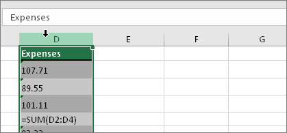
Select a column with this problem. If you don’t want to convert the whole column, you can select one or more cells instead. Just be sure the cells you select are in the same column, otherwise this process won’t work. (See «Other ways to convert» below if you have this problem in more than one column.)
2. Click this button
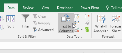
The Text to Columns button is typically used for splitting a column, but it can also be used to convert a single column of text to numbers. On the Data tab, click Text to Columns.
3. Click Apply
The rest of the Text to Columns wizard steps are best for splitting a column. Since you’re just converting text in a column, you can click Finish right away, and Excel will convert the cells.
4. Set the format

Press CTRL + 1 (or  + 1 on the Mac). Then select any format.
Note: If you still see formulas that are not showing as numeric results, then you may have Show Formulas turned on. Go to the Formulas tab and make sure Show Formulas is turned off.
Other ways to convert:
You can use the VALUE function to return just the numeric value of the text.
1. Insert a new column
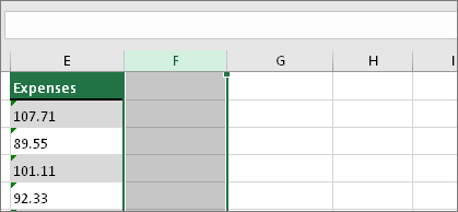
Insert a new column next to the cells with text. In this example, column E contains the text stored as numbers. Column F is the new column.
2. Use the VALUE function
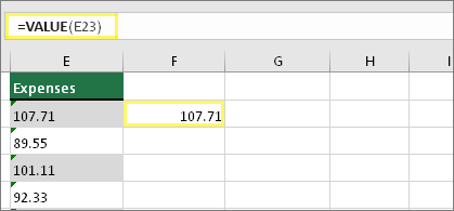
In one of the cells of the new column, type =VALUE() and inside the parentheses, type a cell reference that contains text stored as numbers. In this example it’s cell E23.
3. Rest your cursor here
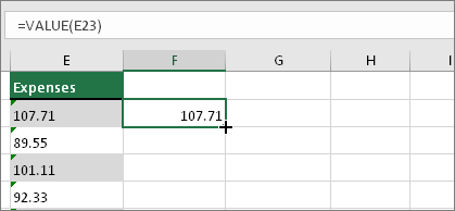
Now you’ll fill the cell’s formula down, into the other cells. If you’ve never done this before, here’s how to do it: Rest your cursor on the lower-right corner of the cell until it changes to a plus sign.
4. Click and drag down
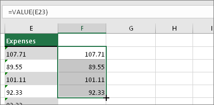
Click and drag down to fill the formula to the other cells. After that’s done, you can use this new column, or you can copy and paste these new values to the original column. Here’s how to do that: Select the cells with the new formula. Press CTRL + C. Click the first cell of the original column. Then on the Home tab, click the arrow below Paste, and then click Paste Special > Values.
If the steps above didn’t work, you can use this method, which can be used if you’re trying to convert more than one column of text.
-
Select a blank cell that doesn’t have this problem, type the number 1 into it, and then press Enter.
-
Press CTRL + C to copy the cell.
-
Select the cells that have numbers stored as text.
-
On the Home tab, click Paste > Paste Special.
-
Click Multiply, and then click OK. Excel multiplies each cell by 1, and in doing so, converts the text to numbers.
-
Press CTRL + 1 (or
 + 1 on the Mac). Then select any format.

Related topics
Replace a formula with its result
Top ten ways to clean your data
CLEAN function
Need more help?
How to save a number as a String in Excel?
When I try to enter a number, 00112233, Excel automatically formats it as 112233 and saving it as number. But I want the preceeding 0’s not to be truncated and save the number as string.
As a workaround I’m using quotes («») to save the actual string.
Any suggestion…??
asked Aug 8, 2013 at 9:56
![]()
Gokul Nath KPGokul Nath KP
15.3k24 gold badges88 silver badges125 bronze badges
If you put a single quote in front of the number, it will be stored as text.
answered Aug 8, 2013 at 9:58
![]()
0
If you pre-format the input cells with TEXT format you can just enter 00112233 or whatever and it will display as entered and be stored as text. To do that select a cell or range of cells and right click — in dialog box choose "Format Cells" and then in the next box choose Number > Text
Note you can’t change to TEXT format after input, or rather you can change the format but it has no effect!
answered Aug 8, 2013 at 10:08
![]()
barry houdinibarry houdini
45.5k8 gold badges63 silver badges80 bronze badges
You need to use single quotes to keep it as text:
'00112233
Will store 00112233 in the cell.
Otherwise, if you have many cells already in number format, and you need them to be in text format with 8 digits (including zeros), you can use the formula on the data:
=text(A1,"00000000")
(there are 8 zeros there)
Then, copy the column containing the formula, paste in place as values (Paste Special > Values) and delete the previous column.
answered Aug 8, 2013 at 10:00
![]()
JerryJerry
70.1k13 gold badges99 silver badges143 bronze badges
|
МЕНЮ САЙТА
КАТЕГОРИИ РАЗДЕЛА ОПРОСЫ |
Число сохранено как текст или Почему не считается сумма?
Добавлять комментарии могут только зарегистрированные пользователи. [ Регистрация | Вход ] |
How many times have you encountered the “Numbers Stored as text” error in your data sets? It interferes with your LOOKUP and MATCH functions, and arithmetic calculations. Excel has a Convert to Number functionality to help with this situation, but it could be a lot better. You have to deal with your columns one at a time, sometimes one cell at a time. Also, I noticed that if the dataset is huge, excel takes a lot of time to push through; occasionally, it is so slow that you can see the cells getting updated one by one.

A quick way to deal with this is to create a temporary column and use the Value function. You may get #Value errors if the string does not represent a numeric value. I use the following formula to do the trick:
=IFERROR(A1*1,TRIM(A1))
This converts all the numbers to “numbers”, trims the text and takes care of the #Value errors if any. You can Copy-Paste-Special-Values over the existing column, and remove the temporary column if you want. This technique works if you have only the Unique Identifier column interfering with your lookups. Imagine your entire database imported into excel as text (with that annoying singe quote in front), you’d be surprised how often that happens. I bet you would not have the patience to set up temporary columns for every field, would you?
I ran into this problem very often, so I buckled down and started thinking of ways to automatically clean up the columns. My first instinct was to deal with the problem one cell at a time. I created a user defined function that cleans up one cell, and then ran a For Each loop through all the cells in a range. This method was extremely slow, even slower than the built-in Convert To Number function. Then I figured using Arrays would speed things up immensely. And that is when I realized something amazing; a single line solved this entire problem:
Selection.Value = Selection.Value
This got the job done in a flash. It automatically got rid all the Convert To Number errors. Who knew excel was already programmed to automatically do this right? If only Microsoft thought to give users the ability to call it at will. However, note that this does not trim cells, and it does not handle dates well. Also, this wont work if you set the Cell’s Number Format to Text.
I ironed out the issues and wrote a sub that trims string, handles dates well and changes Case (Lower/Upper/Proper if you need it to).
Sub AutoTrim(Optional ByRef WhichRange As Range, _
    Optional ByVal ChangeCase As Boolean = False, _
    Optional ByVal ChangeCaseOption As VbStrConv = vbProperCase)

'Declare Sub Level Variables and Objects
Dim MessageAnswer As VbMsgBoxResult
Dim EachRange As Range
Dim TempArray As Variant
Dim RowCounter As Long
Dim ColCounter As Long

'Use the Active Selection if the user did not pass a Range Object to the
'WhichRange Argument
If WhichRange Is Nothing Then
    Set WhichRange = Application.Selection
End If

'If the Range has formulas, it will be converted into values
'Therefore, ask user for permission to proceed
If RangeHasFormulas(WhichRange) Then
    MessageAnswer = MsgBox("Some of the cells contain formulas. " _
        & "Would you like to proceed?", _
        vbQuestion + vbYesNo, "Struggling To Excel")
    If MessageAnswer = vbNo Then Exit Sub
End If

'Loop through each area, So we can loop through all the _
'rectangular boxes
For Each EachRange In WhichRange.Areas
    TempArray = EachRange.Value2
    'If Each range were a single cell, then EachRange.Value
    'would not be an array. Consequently, we have to deal with both
    'these situations separately
    If IsArray(TempArray) Then
        For RowCounter = LBound(TempArray, 1) To UBound(TempArray, 1)
            For ColCounter = LBound(TempArray, 2) To UBound(TempArray, 2)
                'First Check if it is a date
                'Excel Confuses mm/dd/yyyy and dd/mm/yyyy when we just use the
                'Selection.Value = Selection.Value technique. Copy Paste Special
                'Multiply by 1, also suffers from this problem.
                If IsDate(TempArray(RowCounter, ColCounter)) Then
                    TempArray(RowCounter, ColCounter) = _
                        CDate(TempArray(RowCounter, ColCounter))
                Else
                    'Check if it is a number
                    If IsNumeric(TempArray(RowCounter, ColCounter)) Then
                        'Convert it into a Double Variable if it is a number
                        TempArray(RowCounter, ColCounter) = _
                            CDbl(TempArray(RowCounter, ColCounter))
                    Else
                        'Otherwise it is Text. Trim it. I am using Excel's trim
                        'function because it clears double spaces also.
                        TempArray(RowCounter, ColCounter) = _
                            Application.Trim(TempArray(RowCounter, ColCounter))
                        'Finally, Change Case if the user wants to
                        If ChangeCase Then
                            TempArray(RowCounter, ColCounter) = StrConv( _
                            TempArray(RowCounter, ColCounter), ChangeCaseOption)
                        End If
                    End If
                End If

            Next ColCounter
        Next RowCounter
    Else
        'Deal with Single Cells separately
        If IsDate(TempArray) Then
            TempArray = CDate(TempArray)
        Else
            If IsNumeric(TempArray) Then
                TempArray = CDbl(TempArray)
            Else
                TempArray = Application.Trim(TempArray)
                If ChangeCase Then
                    TempArray = StrConv(TempArray, ChangeCaseOption)
                End If
            End If
        End If
    End If
    EachRange.Value2 = TempArray
Next EachRange

End Sub
All you need to do now is select your entire Database, just run this macro, sit back and relax.
Update
- Another popular solution to this problem is to just type “1” in any cell; copy it; and paste-special-value it with the Multiply operator. While this handles Numbers like a charm, it fails to convert dates properly.
- I heard complaints that my code did not handle numbers with commas and decimal points. Consequently I amended the code.
- The macro now uses the following logic:
- First Check if the string is a date. If it is, apply the CDate function.
- Else, check if it the string is Numeric, if It is, apply the CDbl function. This function takes care of the numbers with commas and decimal points.
- If the string is neither a date, nor a number, it must be a string. Therefore, Trim it with Excel’s trim function. I chose to use Excel’s trim function, because it also removes double spaces.
Download

Let me know how you like it. I added a bunch of cover macros in there that illustrates how this sub could be used. There is a sheet named JustValues that has a very crude sample data set. I have copy pasted it in the Test sheet for you to try the cover macros.
I have not tried this macro on a system that uses the m/d/yyyy date system, do let me know if it doesn’t work on your computer. Also if you have dates in the d/m/yy format, you would benefit from reading this article.
Bonus
I had to write a small supporting function that determines if any of the cells in a range have formulas in it. You may need to use something like this in your applications.
Function RangeHasFormulas(ByRef WhichRange As Range) _
    As Boolean

'Declare Function Level Variables
Dim TempVar As Variant

'initialize Variables
TempVar = WhichRange.HasFormula

'Check if the Variant Variable is Null (This avoids an error)
If IsNull(TempVar) Then
    'If Null, some cells have Formulas
    RangeHasFormulas = True
Else
    If TempVar = True Then
        'If True, all cells have Formulas
        RangeHasFormulas = True
    Else
        'If False, none of the cells have formulas
        RangeHasFormulas = False
    End If
End If

End Function
Excel is a great tool which can be used for data entry, as a database, and to analyze data and create dashboards and reports.
While most of the in-built features and default settings are meant to be useful and save time for the users, sometimes, you may want to change things a little.
Converting your numbers into text is one such scenario.
In this tutorial, I will show you some easy ways to quickly convert numbers to text in Excel.
Why Convert Numbers to Text in Excel?
When working with numbers in Excel, it’s best to keep these as numbers only. But in some cases, having a number could actually be a problem.
Lets look at a couple of scenarios where having numbers creates issues for the users.
Keeping Leading Zeros
For example, if you enter 001 in a cell in Excel, you will notice that Excel automatically removes the leading zeros (as it thinks these are unnecessary).
While this is not an issue in most cases (as you wouldn’t leading zeros), in case you do need these then one of the solutions is to convert these numbers to text.
This way, you get exactly what you enter.
One common scenario where you might need this is when you’re working with large numbers – such as SSN or employee ids that have leading zeros.
Entering Large Numeric Values
Do you know that you can only enter a numeric value that is 15 digits long in Excel? If you enter a 16 digit long number, it will change the 16th digit to 0.
So if you are working with SSN, account numbers, or any other type of large numbers, there is a possibility that your input data is automatically being changed by Excel.
And what’s even worse is that you don’t get any prompt or error. It just changes the digits to 0 after the 15th digit.
Again, this is something that is taken care of if you convert the number to text.
Changing Numbers to Dates
This one erk a lot of people (including myself).
Try entering 01-01 in Excel and it will automatically change it to date (01 January of the current year).
So if you enter anything that is a valid date format in Excel, it would be converted to a date.
A lot of people reach out to me for this as they want to enter scores in Excel in this format, but end up getting frustrated when they see dates instead.
Again, changing the format of the cell from number to text will help keep the scores as is.
Now, let’s go ahead and have a look at some of the methods you can use to convert numbers to text in Excel.
Convert Numbers to Text in Excel
In this section, I will cover four different ways you can use to convert numbers to text in Excel.
Not all these methods are the same and some would be more suitable than others depending on your situation.
So let’s dive in!
Adding an Apostrophe
If you manually entering data in Excel and you don’t want your numbers to change the format automatically, here is a simple trick:
Add an apostrophe (‘) before the number
So if you want to enter 001, enter ‘001 (where there is an apostrophe before the number).
And don’t worry, the apostrophe is not visible in the cell. You will only see the number.

When you add an apostrophe before a number, it will change it to text and also add a small green triangle at the top left part of the cell (as shown in th image). It’s Exel way to letting you know that the cell has a number that has been converted to text.
When you add an apostrophe before a number, it tells Excel to consider whatever follows as text.
A quick way to visually confirm whether the cells are formatted as text or not is to see whether the numbers align to the left out to the right. When numbers are formatted as text, they align to the right by default (as they alight to the left)

Even if you add an apostrophe before a number in a cell in Excel, you can still use these as numbers in calculations
Similarly, if you want to enter 01-01, adding an apostrophe would make sure that it doesn’t get changed into a date.
Although this technique works in all cases, it is only useful if you’re manually entering a few numbers in Excel. If you enter a lot of data in a specific range of rows/columns, use the next method.
Converting Cell Format to Text
Another way to make sure that any numeric entry in Excel is considered a text value is by changing the format of the cell.
This way, you don’t have to worry about entering an apostrophe every time you manually enter the data.
You can go ahead entering the data just like you usually do, and Excel would make sure that your numbers are not changed.
Here is how to do this:
- Select the range or rows/column where you would be entering the data
- Click the Home tab

- In the Number group, click on the format drop down

- Select Text from the options that show up

The above steps would change the default formatting of the cells from General to Text.
Now, if you enter any number or any text string in these cells, it would automatically be considered as a text string.
This means that Excel would not automatically change the text you enter (such as truncating the leading zeros or converting entered numbers into dates)
In this example, while I changed the cell formatting first before entering the data, you can also do this with cells that already have data in them.
But remember that if you already had entered numbers that were changed by Excel (such as removing leading zeros or changing text to dates), that won’t come back. You will have to make that data entry again.
Also, keep in mind that cell formatting can change in case you copy and paste some data to these cells. With regular copy-paste, it also copied the formatting from the copied cells. So it’s best to copy and paste values only.
Using the TEXT Function
Excel has an in-built TEXT function that is meant to convert a numeric value to a text value (where you have to specify the format of the text in which you want to get the final result).
This method is useful when you already have a set of numbers and you want to show them in a more readable format or if you want to add some text as suffix or prefix to these numbers.
Suppose you have a set of numbers as shown below, and you want to show all these numbers as five-digit values (which means to add leading zeros to numbers that are less than 5 digits).

While Excel removes any leading zeros in numbers, you can use the below formula to get this:
=TEXT(A2,"00000")

In the above formula, I have used “00000” as the second argument, which tells the formula the format of the output I desire. In this example, 00000 would mean that I need all the numbers to be at least five-digit long.
You can do a lot more with the TEXT function – such as add currency symbol, add prefix or suffix to the numbers, or change the format to have comma or decimals.
Using this method can be useful when you already have the data in Excel and you want to format it in a specific way.
This can also be helpful in saving time when doing manual data entry, where you can quickly enter the data and then use the TEXT function to get it in the desired format.
Using Text to Columns
Another quick way to convert numbers to text in Excel is by using the Text to Columns wizard.
While the purpose of Text to Columns is to split the data into multiple columns, it has a setting that also allows us to quickly select a range of cells and convert all the numbers into text with a few clicks.
Suppose you have a data set is shown below, and you want to convert all the numbers in columns A into text.
Below are the steps to do this:
- Select the numbers in Column A
- Click the Data tab

- Click on the Text to Columns icon in the ribbon. This will open the text to columns wizard this will open the text to column wizard
- In Step 1 of 3, click the Next button
- In Step 2 of 3, click the Next button
- In Step 3 of 3, under the ‘Column data format’ options, select Text

- Click on Finish
The above steps would instantly convert all these numbers in Column A into text. You notice that the numbers would now be aligned to the right (indicating that the cell content is text).

There would also be a small green triangle at the top left part of the cell, which is a way Excel informs you that there are numbers that are stored as text.
So these are four easy ways that you can use to quickly convert numbers to text in Excel.
In case you only want this for a few cells where you would be manually entering the data, I suggest you use the apostrophe method. If you need to do data entry for more than a few cells, you can try changing the format of the cells from General to Text.
And in case you already have the numbers in Excel and you want to convert them to text, you can use the TEXT formula method or the Text to Columns method I covered in this tutorial.
I hope you found this tutorial useful.
Other Excel tutorials you may also like:
- Convert Text to Numbers in Excel
- How to Convert Serial Numbers to Dates in Excel
- Convert Date to Text in Excel – Explained with Examples
- How to Convert Formulas to Values in Excel
- Convert Time to Decimal Number in Excel
- How to Convert Inches to MM, CM, or Feet in Excel?
- Convert Scientific Notation to Number or Text in Excel
- Separate Text and Numbers in Excel
Table of Contents
- INTRODUCTION
- HOW TEXT IS HANDLED IN EXCEL?
- NUMBER STORED AS TEXT PROBLEM IN EXCEL
- CONCEPT:
- HOW TO RECOGNIZE IF THE NUMBER IS STORED AS TEXT?
- HOW TO CONVERT NUMBER STORED AS TEXT , BACK TO NUMBER?
INTRODUCTION
Whenever we prepare any report in excel, we have two constituents in any report.
The Text portion and the Numerical portion.
But just storing the text and numbers doesn’t make the super reports. Many times we need to automate the process in the reports to minimize the effort and improve the accuracy.
Many functions are provided by the Excel which work on Text and give us the useful output as well. But few problems are still left on which we need to apply some tricks with the available tools.
In this articles , we are going to learn to get rid of the problem called NUMBER STORED AS TEXT.
HOW TEXT IS HANDLED IN EXCEL?
TEXT is simply the group of characters and strings of characters which convey the information about the different data and numbers in Excel. Every character is connected with a code [ANSI].
Text comprises of the individual entity character which is the smallest bit which would be found in Excel.We can perform the operations on the strings[Text] or the characters.
Characters are not limited to A to Z or a to z but many symbols are also included in this which we would see in the later part of the article.
TEXT IS AN INACTIVE NUMBER TYPE[FORMAT] IN EXCEL. ANYTHING STORED AS TEXT [NUMBER OR DATE] WON’T RESPOND TO ANY STANDARD FORMULAS OR FUNCTIONS BUT SPECIALLY DESIGNED TEXT FUNCTIONS. [EXCEPTIONS DO OCCUR IN CASE OF NUMBERS]
If we need to make anything inactive, such as Date to be non responding to the calculation, we put it as a text. Similarly if we want to avoid any calculations for a number it needs to be put as a text.
CONCEPT:
Have you ever noticed that your cell contain a number [ visibly number] but it is not responding to your formulas or functions as expected.
Most probably it is because of the format of the cell or NUMBER TYPE OF THE CELL.
Out of many problems with the formatting of the cell , we are going to focus on the one called NUMBER STORED AS TEXT.
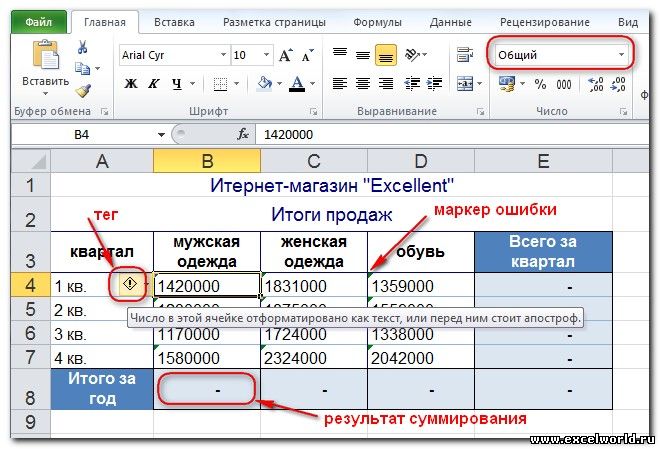
Sometimes or we say most of the time when we copy any number from somewhere or get the data through any channel, we get this problem that the NUMBER IS VISIBLE AS A NUMBER BUT THE FORMAT IS TEXT. The problem with such numbers is that they won’t respond to our calculations. Look at the picture below.

As we can see from the picture above that the text is not responding to the functions. [Although Excel is smart enough to do the simple tasks like addition , subtraction etc. even with the number stored as text]
HOW TO RECOGNIZE IF THE NUMBER IS STORED AS TEXT?
That is pretty simple. Excel itself marks it by a small TRIANGLE AT THE LEFT UPPER CORNER.

HOW TO CONVERT NUMBER STORED AS TEXT , BACK TO NUMBER?
Just click the TRIANGLE MENTIONED ABOVE.

Excel will give you a number of options like

Choose CONVERT TO NUMBER option and all the numbers which were earlier stored as text will be changed to numbers.
Now, they’ll respond to the functions and formulas normally.

Skip to content
When importing data from external sources you may find that your number values unexpectedly import as text.
It’s usually obvious when this happens – the numbers are left-aligned.
The cells may look like a number, but Excel thinks that they are text.
You’ll find that you can’t perform calculations against “text-numbers”. For the picture below, if I used the formula =SUM(A1:A10) then the result would be 0.
Excel 2002 (Excel XP) made some advances in this area by way of automatic error-checking (aka the Green Triangle).
You can quickly convert the cell to a proper number by highlighting your list of misbehaving numbers, click the exclaimation mark and choose ‘Convert to Number’ from the dropdown.

For those of you running a version of Excel less than 2002, the trick I use goes as follows:
1. Copy a Blank Cell (or a cell containing the number 0)
2. Select your list of text-numbers
3. Choose Paste Special from the Edit menu.
4. Paste=Values, Operation=Add
By applying a math operation on the text-numbers, the result is a number!
Sure beats pressing “F2 Enter” 100 times like I used to.
Преобразование чисел-как-текст в нормальные числа
Если для каких-либо ячеек на листе был установлен текстовый формат (это мог сделать пользователь или программа при выгрузке данных в Excel), то введенные потом в эти ячейки числа Excel начинает считать текстом. Иногда такие ячейки помечаются зеленым индикатором, который вы, скорее всего, видели:

Причем иногда такой индикатор не появляется (что гораздо хуже).
В общем и целом, появление в ваших данных чисел-как-текст обычно приводит к большому количеству весьма печальных последствий:
Особенно забавно, что естественное желание просто изменить формат ячейки на числовой — не помогает. Т.е. вы, буквально, выделяете ячейки, щелкаете по ним правой кнопкой мыши, выбираете Формат ячеек (Format Cells), меняете формат на Числовой (Number), жмете ОК — и ничего не происходит! Совсем!
Возможно, «это не баг, а фича», конечно, но нам от этого не легче. Так что давайте-к рассмотрим несколько способов исправить ситуацию — один из них вам обязательно поможет.
Способ 1. Зеленый уголок-индикатор
Если на ячейке с числом с текстовом формате вы видите зеленый уголок-индикатор, то считайте, что вам повезло. Можно просто выделить все ячейки с данными и нажать на всплывающий желтый значок с восклицательным знаком, а затем выбрать команду Преобразовать в число (Convert to number):

Все числа в выделенном диапазоне будут преобразованы в полноценные.
Если зеленых уголков нет совсем, то проверьте — не выключены ли они в настройках вашего Excel (Файл — Параметры — Формулы — Числа, отформатированные как текст или с предшествующим апострофом).
Способ 2. Повторный ввод
Если ячеек немного, то можно поменять их формат на числовой, а затем повторно ввести данные, чтобы изменение формата вступило-таки в силу. Проще всего это сделать, встав на ячейку и нажав последовательно клавиши F2 (вход в режим редактирования, в ячейке начинает мигаеть курсор) и затем Enter. Также вместо F2 можно просто делать двойной щелчок левой кнопкой мыши по ячейке.
Само-собой, что если ячеек много, то такой способ, конечно, не подойдет.
Способ 3. Формула
Можно быстро преобразовать псевдочисла в нормальные, если сделать рядом с данными дополнительный столбец с элементарной формулой:

Двойной минус, в данном случае, означает, на самом деле, умножение на -1 два раза. Минус на минус даст плюс и значение в ячейке это не изменит, но сам факт выполнения математической операции переключает формат данных на нужный нам числовой.
Само-собой, вместо умножения на 1 можно использовать любую другую безобидную математическую операцию: деление на 1 или прибавление-вычитание нуля. Эффект будет тот же.
Способ 4. Специальная вставка
Этот способ использовали еще в старых версиях Excel, когда современные эффективные менеджеры под стол ходили зеленого уголка-индикатора еще не было в принципе (он появился только с 2003 года). Алгоритм такой:
- в любую пустую ячейку введите 1
- скопируйте ее
- выделите ячейки с числами в текстовом формате и поменяйте у них формат на числовой (ничего не произойдет)
- щелкните по ячейкам с псевдочислами правой кнопкой мыши и выберите команду Специальная вставка (Paste Special) или используйте сочетание клавиш Ctrl+Alt+V
- в открывшемся окне выберите вариант Значения (Values) и Умножить (Multiply)

По-сути, мы выполняем то же самое, что и в прошлом способе — умножение содержимого ячеек на единицу — но не формулами, а напрямую из буфера.
Способ 5. Текст по столбцам
Если псеводчисла, которые надо преобразовать, вдобавок еще и записаны с неправильными разделителями целой и дробной части или тысяч, то можно использовать другой подход. Выделите исходный диапазон с данными и нажмите кнопку Текст по столбцам (Text to columns) на вкладке Данные (Data). На самом деле этот инструмент предназначен для деления слипшегося текста по столбцам, но, в данном случае, мы используем его с другой целью.
Пропустите первых два шага нажатием на кнопку Далее (Next), а на третьем воспользуйтесь кнопкой Дополнительно (Advanced). Откроется диалоговое окно, где можно задать имеющиеся сейчас в нашем тексте символы-разделители:

После нажатия на Готово Excel преобразует наш текст в нормальные числа.
Способ 6. Макрос
Если подобные преобразования вам приходится делать часто, то имеет смысл автоматизировать этот процесс при помощи несложного макроса. Нажмите сочетание клавиш Alt+F11 или откройте вкладку Разработчик (Developer) и нажмите кнопку Visual Basic. В появившемся окне редактора добавьте новый модуль через меню Insert — Module и скопируйте туда следующий код:
Sub Convert_Text_to_Numbers()
    Selection.NumberFormat = "General"
    Selection.Value = Selection.Value
End Sub
Теперь после выделения диапазона всегда можно открыть вкладку Разрабочик — Макросы (Developer — Macros), выбрать наш макрос в списке, нажать кнопку Выполнить (Run) — и моментально преобразовать псевдочисла в полноценные.
Также можно добавить этот макрос в личную книгу макросов, чтобы использовать позднее в любом файле.
P.S.
С датами бывает та же история. Некоторые даты тоже могут распознаваться Excel’ем как текст, поэтому не будет работать группировка и сортировка. Решения — те же самые, что и для чисел, только формат вместо числового нужно заменить на дату-время.
Ссылки по теме
- Деление слипшегося текста по столбцам
- Вычисления без формул специальной вставкой
- Преобразование текста в числа с помощью надстройки PLEX
Numbers that are stored as text can cause unexpected results, especially when you use these cells in Excel functions such as SUM and AVERAGE because these functions ignore cells that have text values in them. So you need to convert numbers stored as text to numbers.
How do I change my number stored as text to number?
Select the Excel cells and then click the trace error button and select the convert to numbers option. Or, follow the methods below if that button is not available.
You can follow any one of these methods below to convert numbers stored as text to numbers in Microsoft Excel:
- Using the Text to column button
- Using Value function
- Changing the format
- Use Paste Special and multiply
1] Using the Text to column button

Select the column or select one or more cells, ensure that the cells you have selected are in the same column, or else the process won’t work.
Then click the Data tab and click the Text to column button.
A Convert text to column wizard dialog box appears.
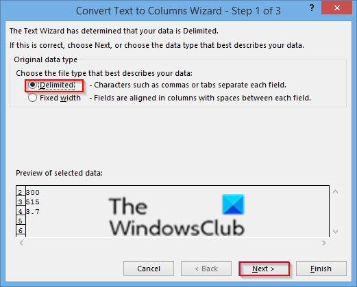
Select the Delimited option, then click Next.
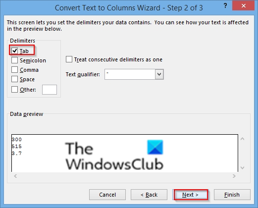
Select Tab as the delimiter, then click Next.
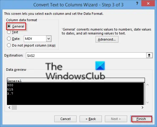
Select General as the column data format, then click Finish.
2] Using Value function
You can use the Value function to return the numeric value of the text.
Select a new cell in a different column.
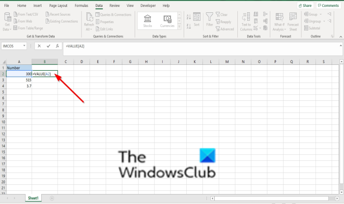
Type the formula =Value() and inside the parentheses, type a cell reference that contains text stored as numbers. In this example, it’s cell A2.
Press Enter.
Now place the cursor at the lower right corner of the cell and drag the fill handle down to fill the formula for the other cells.
Then copy and paste the new values to the original cell column.

To copy and paste the values to the Original column, select the cells with the new formula. Press CTRL + C. Then click the first cell of the original column. Then on the Home tab, click the arrow below Paste, and click Paste special.
On the Paste Special dialog box, click Values.
3] Changing the format
Select a cell or cells.
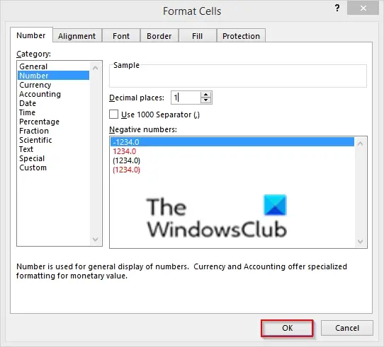
Then Press Ctrl + 1 button to open a Format Cells dialog box.
Then select any format.
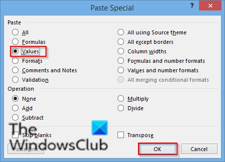
4] Use Paste special and multiply
If you are converting more than one column of text to numbers, this is an excellent method to use.
Select a blank cell and type 1 into it.
Then press Press CTRL + C to copy the cell.
Then select the cells stored as text.
On the Home tab, click the arrow below Paste, and then click Paste Special.
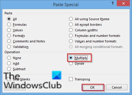
On the Paste Special dialog box, click Multiply.
Then click OK.
Microsoft Excel multiplies each cell by 1, and in doing so, converts the text to numbers.
We hope this tutorial helps you understand how to convert numbers stored as text to numbers in Excel.
Why is my number stored as text in Excel?
Excel doesn’t convert numbers written in text into digits if you import data from another source because of the default setting. That being said, even if you copy data from the internet and paste it into the Excel spreadsheet, you can find numbers in the text. You can follow the aforementioned steps to convert the numbers from text to digits.
How do I ignore all numbers stored as text in Excel?
To ignore all numbers stored as text, you need to open the Data tab and select the Text to Columns option. Then, select the Delimited option from the Convert Text to Columns wizard. Remove the tick from all the checkboxes and select the General option in the Column data format panel. Finally, click the Finish button to make the conversion happen.
If you have questions about the tutorial, let us know in the comments.