
Содержание
- VBA Row Count
- Excel VBA Row Count
- How to Count Rows in VBA?
- Example #1
- Example #2
- Example #3 – Find Last Used Row
- Things to Remember
- Recommended Articles
- How To Get Row Number By A Single Click Using VBA In Microsoft Excel 2010
- Refer to Rows and Columns
- About the Contributor
- Support and feedback
- Excel VBA Ranges and Cells
- Ranges and Cells in VBA
- Cell Address
- A1 Notation
- R1C1 Notation
- Range of Cells
- A1 Notation
- R1C1 Notation
- Writing to Cells
- Reading from Cells
- Non Contiguous Cells
- VBA Coding Made Easy
- Intersection of Cells
- Offset from a Cell or Range
- Offset Syntax
- Offset from a cell
- Offset from a Range
- Setting Reference to a Range
- Resize a Range
- Resize Syntax
- OFFSET vs Resize
- All Cells in Sheet
- UsedRange
- CurrentRegion
- Range Properties
- Last Cell in Sheet
- Last Used Row Number in a Column
- Last Used Column Number in a Row
- Cell Properties
- Common Properties
- Cell Font
- Copy and Paste
- Paste All
- Paste Special
- AutoFit Contents
- More Range Examples
- For Each
- Range Address
- Range to Array
- Array to Range
- Sum Range
- Count Range
- VBA Code Examples Add-in
VBA Row Count


Excel VBA Row Count
In VBA programming, referring to rows is most important as well, and counting them is one thing you must be aware of when it comes to VBA coding. We can get a lot of value if we understand the importance of counting rows with data in the worksheet. This article will show you how to count rows using VBA coding.
You are free to use this image on your website, templates, etc., Please provide us with an attribution link How to Provide Attribution? Article Link to be Hyperlinked
For eg:
Source: VBA Row Count (wallstreetmojo.com)
Table of contents
How to Count Rows in VBA?
Example #1
Look at the below data in Excel.

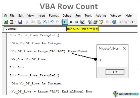
From the above data, we need to identify how many rows are there from the range A1 to A8. So first, define the variable as an Integer to store the number of rows.
Code:

We will assign row numbers for this variable, so enter the variable name and the equal sign.
Code:

Code:

Once we supply the range, we need to count the number of rows, so choose the ROWS property of the RANGE object.
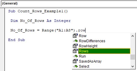
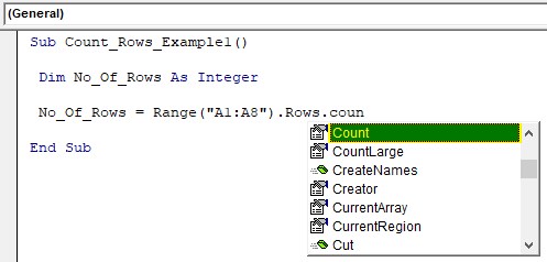
We are counting several rows in the RANGE object’s ROWS property, so choose the “COUNT” property now.
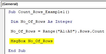
Now in the message box, show the value of the variable.
Code:
Now, run the code and see the count of rows of the supplied range of cells.

There are 8 rows supplied for the range, so the row count is 8 in the message box.
Example #2
We have other ways of counting rows as well. For the above method, we need to supply a range of cells, showing the number of rows selected.
But imagine the scenario where we need to find the last use of any column. For example, take the same data as seen above.
To move to the last used cell from cell A1, we press the shortcut excel key Shortcut Excel Key An Excel shortcut is a technique of performing a manual task in a quicker way. read more “Ctrl + Down Arrow,” so it will take you to the last cell before the empty cell.
First, supply the cell as A1 using the RANGE object.
Code:
Look there with the END key. We can see all the arrow keys like “xlDown, xlToLeft, xlToRight, and xlUp” since we need to move down and use the “xlDown” option.
Code:
Code:

So in rows, we have data.
Example #3 – Find Last Used Row
Finding the last used row is important to decide how many times the loop has to run. Also, in the above method, the last row stops to select if there is any breakpoint cell. So in this method, we can find the last used row without any problems.
Code:
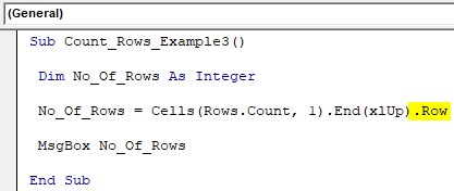
Now, we need to mention the row number to start with. The problem here is we are not sure how many rows of data we have so that we can go straight to the last row of the worksheet, for this mention, ROWS.COUNT property.
Code:
Next, we need to mention in which column we are finding the last used row, so in this case, we are finding it in the first column, so mention 1.
Code:
At this moment, it will take you to the last cell of the first column. We need to move upwards to the last used cell from there onwards, so use the End(xlUp) property.
Code:
So, this will take you to the last used cell of column 1, and in this cell, we need the row number, so use the ROW property to get the row number.
Code:
Things to Remember
- The COUNT will give several rows in the worksheet.
- If you have a range, then it will give several rows selected in the range.
- The ROW property will return the active cell row number.
Recommended Articles
This article has been a guide to VBA Row Count. Here, we discuss how to count used rows in Excel using VBA coding, practical examples, and a downloadable Excel template. You may learn more about Excel from the following articles: –
Источник
How To Get Row Number By A Single Click Using VBA In Microsoft Excel 2010
In this article, you will learn how to get row number by a single click.
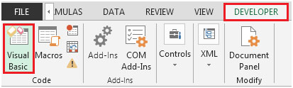
Click on Developer tab
From Code group, select Visual Basic
Enter the following code in the current worksheet (sheet1 in our example)
Private Sub Worksheet_SelectionChange(ByVal Target As Range)
Dim rownumber As Integer
rownumber = ActiveCell.Row
If ActiveCell.Value <> «» Then
MsgBox «You have clicked on row number » & rownumber
End If
End Sub
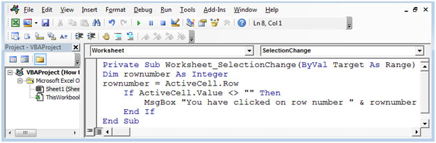
The SelectionChange event will get activated every time the user selects any cell & it will give us the row number of the selected cell. If active cell is empty then, the code will not run.
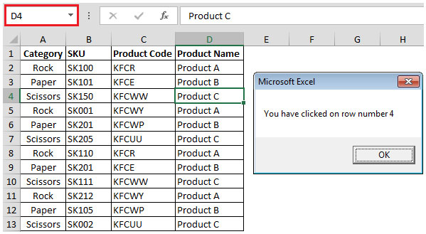
In above snapshot, you can see the formula bar contains cell D4 & hence the row number is 4.
If we select cell A1, and then we get the row number as 1. Refer below shown snapshot
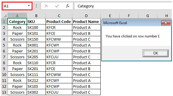
In this way, you can get the row number of the selected cell, using VBA code.
Источник
Refer to Rows and Columns
Use the Rows property or the Columns property to work with entire rows or columns. These properties return a Range object that represents a range of cells. In the following example, Rows(1) returns row one on Sheet1. The Bold property of the Font object for the range is then set to True.
The following table illustrates some row and column references using the Rows and Columns properties.
| Reference | Meaning |
|---|---|
| Rows(1) | Row one |
| Rows | All the rows on the worksheet |
| Columns(1) | Column one |
| Columns(«A») | Column one |
| Columns | All the columns on the worksheet |
To work with several rows or columns at the same time, create an object variable and use the Union method, combining multiple calls to the Rows or Columns property. The following example changes the format of rows one, three, and five on worksheet one in the active workbook to bold.
Sample code provided by: Dennis Wallentin, VSTO & .NET & Excel This example deletes the empty rows from a selected range.
This example deletes the empty columns from a selected range.
About the Contributor
Dennis Wallentin is the author of VSTO & .NET & Excel, a blog that focuses on .NET Framework solutions for Excel and Excel Services. Dennis has been developing Excel solutions for over 20 years and is also the coauthor of «Professional Excel Development: The Definitive Guide to Developing Applications Using Microsoft Excel, VBA and .NET (2nd Edition).»
Support and feedback
Have questions or feedback about Office VBA or this documentation? Please see Office VBA support and feedback for guidance about the ways you can receive support and provide feedback.
Источник
Excel VBA Ranges and Cells
In this Article
Ranges and Cells in VBA
Excel spreadsheets store data in Cells. Cells are arranged into Rows and Columns. Each cell can be identified by the intersection point of it’s row and column (Exs. B3 or R3C2).
An Excel Range refers to one or more cells (ex. A3:B4)
Cell Address
A1 Notation
In A1 notation, a cell is referred to by it’s column letter (from A to XFD) followed by it’s row number(from 1 to 1,048,576). This is called a cell address.
In VBA you can refer to any cell using the Range Object.
R1C1 Notation
In R1C1 Notation a cell is referred by R followed by Row Number then letter ‘C’ followed by the Column Number. eg B4 in R1C1 notation will be referred by R4C2. In VBA you use the Cells Object to use R1C1 notation:
Range of Cells
A1 Notation
To refer to a more than one cell use a “:” between the starting cell address and last cell address. The following will refer to all the cells from A1 to D10:
R1C1 Notation
To refer to a more than one cell use a “,” between the starting cell address and last cell address. The following will refer to all the cells from A1 to D10:
Writing to Cells
To write values to a cell or contiguous group of cells, simple refer to the range, put an = sign and then write the value to be stored:
Reading from Cells
To read values from cells, simple refer to the variable to store the values, put an = sign and then refer to the range to be read:
Note: To store values from a range of cells, you need to use an Array instead of a simple variable.
Non Contiguous Cells
To refer to non contiguous cells use a comma between the cell addresses:
VBA Coding Made Easy
Stop searching for VBA code online. Learn more about AutoMacro — A VBA Code Builder that allows beginners to code procedures from scratch with minimal coding knowledge and with many time-saving features for all users!

Intersection of Cells
To refer to non contiguous cells use a space between the cell addresses:
Offset from a Cell or Range
Using the Offset function, you can move the reference from a given Range (cell or group of cells) by the specified number_of_rows, and number_of_columns.
Offset Syntax
Offset from a cell
Offset from a Range
Setting Reference to a Range
To assign a range to a range variable: declare a variable of type Range then use the Set command to set it to a range. Please note that you must use the SET command as RANGE is an object:
Resize a Range
Resize method of Range object changes the dimension of the reference range:
Top-left cell of the Resized range is same as the top-left cell of the original range
Resize Syntax
OFFSET vs Resize
Offset does not change the dimensions of the range but moves it by the specified number of rows and columns. Resize does not change the position of the original range but changes the dimensions to the specified number of rows and columns.
All Cells in Sheet
The Cells object refers to all the cells in the sheet (1048576 rows and 16384 columns).
UsedRange
UsedRange property gives you the rectangular range from the top-left cell used cell to the right-bottom used cell of the active sheet.
CurrentRegion
CurrentRegion property gives you the contiguous rectangular range from the top-left cell to the right-bottom used cell containing the referenced cell/range.
Range Properties
You can get Address, row/column number of a cell, and number of rows/columns in a range as given below:
Last Cell in Sheet
You can use Rows.Count and Columns.Count properties with Cells object to get the last cell on the sheet:
Last Used Row Number in a Column
END property takes you the last cell in the range, and End(xlUp) takes you up to the first used cell from that cell.
Last Used Column Number in a Row
END property takes you the last cell in the range, and End(xlToLeft) takes you left to the first used cell from that cell.
You can also use xlDown and xlToRight properties to navigate to the first bottom or right used cells of the current cell.
Cell Properties
Common Properties
Here is code to display commonly used Cell Properties
Cell Font
Cell.Font object contains properties of the Cell Font:
Copy and Paste
Paste All
Ranges/Cells can be copied and pasted from one location to another. The following code copies all the properties of source range to destination range (equivalent to CTRL-C and CTRL-V)
Paste Special
Selected properties of the source range can be copied to the destination by using PASTESPECIAL option:
Here are the possible options for the Paste option:
AutoFit Contents
Size of rows and columns can be changed to fit the contents using AutoFit:
More Range Examples
It is recommended that you use Macro Recorder while performing the required action through the GUI. It will help you understand the various options available and how to use them.
For Each
It is easy to loop through a range using For Each construct as show below:
At each iteration of the loop one cell in the range is assigned to the variable cell and statements in the For loop are executed for that cell. Loop exits when all the cells are processed.
Sort is a method of Range object. You can sort a range by specifying options for sorting to Range.Sort. The code below will sort the columns A:C based on key in cell C2. Sort Order can be xlAscending or xlDescending. Header:= xlYes should be used if first row is the header row.
Find is also a method of Range Object. It find the first cell having content matching the search criteria and returns the cell as a Range object. It return Nothing if there is no match.
Use FindNext method (or FindPrevious) to find next(previous) occurrence.
Following code will change the font to “Arial Black” for all cells in the range which start with “John”:
Following code will replace all occurrences of “To Test” to “Passed” in the range specified:
It is important to note that you must specify a range to use FindNext. Also you must provide a stopping condition otherwise the loop will execute forever. Normally address of the first cell which is found is stored in a variable and loop is stopped when you reach that cell again. You must also check for the case when nothing is found to stop the loop.
Range Address
Use Range.Address to get the address in A1 Style
Use xlReferenceStyle (default is xlA1) to get addres in R1C1 style
This is useful when you deal with ranges stored in variables and want to process for certain addresses only.
Range to Array
It is faster and easier to transfer a range to an array and then process the values. You should declare the array as Variant to avoid calculating the size required to populate the range in the array. Array’s dimensions are set to match number of values in the range.
Array to Range
After processing you can write the Array back to a Range. To write the Array in the example above to a Range you must specify a Range whose size matches the number of elements in the Array.
Use the code below to write the Array to the range D1:D5:
Please note that you must Transpose the Array if you write it to a row.
Sum Range
You can use many functions available in Excel in your VBA code by specifying Application.WorkSheetFunction. before the Function Name as in the example above.
Count Range
Written by: Vinamra Chandra

VBA Code Examples Add-in
Easily access all of the code examples found on our site.
Simply navigate to the menu, click, and the code will be inserted directly into your module. .xlam add-in.
Источник
Excel VBA Row Count
In VBA programming, referring to rows is most important as well, and counting them is one thing you must be aware of when it comes to VBA coding. We can get a lot of value if we understand the importance of counting rows with data in the worksheet. This article will show you how to count rows using VBA coding.
You are free to use this image on your website, templates, etc, Please provide us with an attribution linkArticle Link to be Hyperlinked
For eg:
Source: VBA Row Count (wallstreetmojo.com)
Table of contents
- Excel VBA Row Count
- How to Count Rows in VBA?
- Example #1
- Example #2
- Example #3 – Find Last Used Row
- Things to Remember
- Recommended Articles
- How to Count Rows in VBA?
How to Count Rows in VBA?
You can download this VBA Row Count Excel Template here – VBA Row Count Excel Template
Example #1
To count rowsThere are numerous ways to count rows in Excel using the appropriate formula, whether they are data rows, empty rows, or rows containing numerical/text values. Depending on the circumstance, you can use the COUNTA, COUNT, COUNTBLANK, or COUNTIF functions.read more, we need to use the RANGE object. In this object, we need to use the ROWS object. In this, we need to use the COUNT property.
Look at the below data in Excel.
From the above data, we need to identify how many rows are there from the range A1 to A8. So first, define the variable as an Integer to store the number of rows.
Code:
Sub Count_Rows_Example1()

Dim No_Of_Rows As Integer

End Sub
We will assign row numbers for this variable, so enter the variable name and the equal sign.
Code:
Sub Count_Rows_Example1()

Dim No_Of_Rows As Integer

No_Of_Rows =

End Sub
We need to provide a range of cells, so open the RANGE objectRange is a property in VBA that helps specify a particular cell, a range of cells, a row, a column, or a three-dimensional range. In the context of the Excel worksheet, the VBA range object includes a single cell or multiple cells spread across various rows and columns.read more and supply the range as “A1:A8”.
Code:
Sub Count_Rows_Example1()

Dim No_Of_Rows As Integer

No_Of_Rows = Range("A1:A8")

End Sub
Once we supply the range, we need to count the number of rows, so choose the ROWS property of the RANGE object.
We are counting several rows in the RANGE object’s ROWS property, so choose the “COUNT” property now.
Now in the message box, show the value of the variable.
Code:
Sub Count_Rows_Example1()

Dim No_Of_Rows As Integer

No_Of_Rows = Range("A1:A8").Rows.Count

MsgBox No_Of_Rows

End Sub
Now, run the code and see the count of rows of the supplied range of cells.
There are 8 rows supplied for the range, so the row count is 8 in the message box.
Example #2
We have other ways of counting rows as well. For the above method, we need to supply a range of cells, showing the number of rows selected.
But imagine the scenario where we need to find the last use of any column. For example, take the same data as seen above.
To move to the last used cell from cell A1, we press the shortcut excel keyAn Excel shortcut is a technique of performing a manual task in a quicker way.read more “Ctrl + Down Arrow,” so it will take you to the last cell before the empty cell.
First, supply the cell as A1 using the RANGE object.
Code:
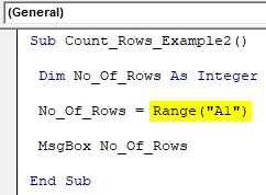
Sub Count_Rows_Example2()

Dim No_Of_Rows As Integer

No_Of_Rows = Range("A1")

MsgBox No_Of_Rows

End Sub
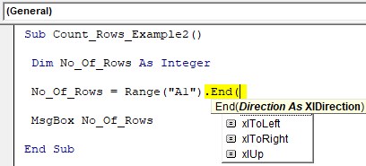
From this cell, we need to move down. We use Ctrl + Down Arrow in the worksheet, but in VBA, we use the END propertyEnd is a VBA statement that can be used in a variety of ways in VBA applications. Anywhere in the code, a simple End statement can be used to instantly end the execution of the code. In procedures, the end statement is used to end a subprocedure or any loop function, such as ‘End if’.read more. Choose this property and open the bracket to see options.
Look there with the END key. We can see all the arrow keys like “xlDown, xlToLeft, xlToRight, and xlUp” since we need to move down and use the “xlDown” option.
Code:
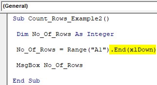
Sub Count_Rows_Example2()

Dim No_Of_Rows As Integer

No_Of_Rows = Range("A1").End(xlDown)

MsgBox No_Of_Rows

End Sub
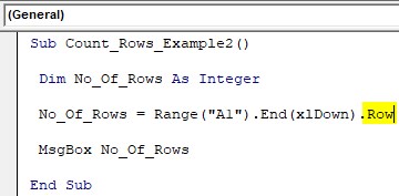
It will take you to the last cell before any break. We need the row number in the active cellThe active cell is the currently selected cell in a worksheet. Active cell in VBA can be used as a reference to move to another cell or change the properties of the same active cell or the cell’s reference provided from the active cell.read more so use the ROW property.
Code:
Sub Count_Rows_Example2()

Dim No_Of_Rows As Integer

No_Of_Rows = Range("A1").End(xlDown).Row

MsgBox No_Of_Rows

End Sub
Now, this will show the last row numberThe End(XLDown) method is the most commonly used method in VBA to find the last row, but there are other methods, such as finding the last value in VBA using the find function (XLDown).read more, which will be the count of the number of rows.
So in rows, we have data.
Example #3 – Find Last Used Row
Finding the last used row is important to decide how many times the loop has to run. Also, in the above method, the last row stops to select if there is any breakpoint cell. So in this method, we can find the last used row without any problems.
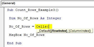
Open CELL propertyCells are cells of the worksheet, and in VBA, when we refer to cells as a range property, we refer to the same cells. In VBA concepts, cells are also the same, no different from normal excel cells.read more.
Code:
Sub Count_Rows_Example3()

Dim No_Of_Rows As Integer

No_Of_Rows = Cells(

MsgBox No_Of_Rows

End Sub
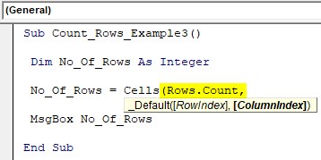
Now, we need to mention the row number to start with. The problem here is we are not sure how many rows of data we have so that we can go straight to the last row of the worksheet, for this mention, ROWS.COUNT property.
Code:
Sub Count_Rows_Example3()

Dim No_Of_Rows As Integer

No_Of_Rows = Cells(Rows.Count,

MsgBox No_Of_Rows

End Sub
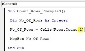
Next, we need to mention in which column we are finding the last used row, so in this case, we are finding it in the first column, so mention 1.
Code:
Sub Count_Rows_Example3()

Dim No_Of_Rows As Integer

No_Of_Rows = Cells(Rows.Count, 1)

MsgBox No_Of_Rows

End Sub
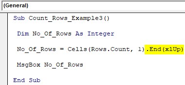
At this moment, it will take you to the last cell of the first column. We need to move upwards to the last used cell from there onwards, so use the End(xlUp) property.
Code:
Sub Count_Rows_Example3()

Dim No_Of_Rows As Integer

No_Of_Rows = Cells(Rows.Count, 1).End(xlUp)

MsgBox No_Of_Rows

End Sub
So, this will take you to the last used cell of column 1, and in this cell, we need the row number, so use the ROW property to get the row number.
Code:
Sub Count_Rows_Example3()

Dim No_Of_Rows As Integer

No_Of_Rows = Cells(Rows.Count, 1).End(xlUp).Row

MsgBox No_Of_Rows

End Sub
Things to Remember
- The COUNT will give several rows in the worksheet.
- If you have a range, then it will give several rows selected in the range.
- The ROW property will return the active cell row number.
Recommended Articles
This article has been a guide to VBA Row Count. Here, we discuss how to count used rows in Excel using VBA coding, practical examples, and a downloadable Excel template. You may learn more about Excel from the following articles: –
- VBA Insert Row
- VBA Delete Row
- VBA StatusBar
- VBA Variable Range
First Cell in Column Function
It is assumed that you’re looking for a VBA function to use in Excel to calculate the first non-empty row of a column (specified by a range).
Features
- The
Volatilemethod marks a user-defined function as volatile. A
volatile function must be recalculated whenever calculation occurs in
any cells on the worksheet. A nonvolatile function is recalculated
only when the input variables change (VBA Help). - At least for the sake of correctness, you have to use
IsEmpty
instead of «» for the reason e.g. if the cell in the resulting row
contains a formula that evaluates to «», it will be ignored. - The Find Method Version uses the Find method to calculate the First Row, which is safer than
the End Version e.g. if you input a value into the first cell of the
column i.e. the result is 1 and you hide the first row, the result of
the End Version will not be 1. - The formula can be inserted in the same column as
SelectRange
Column. In some cases the End Version would not show the correct
result or create a circular reference. ThereforeThisCellis used
in the End version and 0 is returned if no value was found inSelectRangecolumn.
Find Method Version
Function FirstRowFind(SelectRange As Range) As Long

    Application.Volatile

    Dim FirstCell As Range

    With Columns(SelectRange.Column)
        Set FirstCell = .Find("*", .Cells(.Cells.Count), -4123, 1, 2, 1)
    End With

    If Not FirstCell Is Nothing Then
        FirstRowFind = FirstCell.Row
    End If

End Function
Find Method
Instead of
Set FirstCell = .Find("*", .Cells(.Cells.Count), -4123, 1, 2, 1)
you can use
Set FirstCell = .Find("*", .Cells(.Cells.Count), _
        xlFormulas, xlWhole, xlByColumns, xlNext)
or
Set FirstCell = .Find(What:="*", After:=.Cells(.Cells.Count), _
        LookIn:=xlFormulas, LookAt:=xlWhole, _
        SearchOrder:=xlByColumns, SearchDirection:=xlNext)
The parameters for the arguments LookAt(unimportant in this case) and SearchDirection(Default is Next) can be omitted, but since I couldn’t find any difference in efficiency, I didn’t.
Usage in Excel
For Column AB:
=FirstRowFind(AB1)
=FirstRowFind(AB20)
=FirstRowFind(AB17:AH234)
End Version (Not recommended)
Function FirstRowEnd(SelectRange As Range) As Long

    Application.Volatile

    Dim FirstCell As Range

    If Application.ThisCell.Column = SelectRange.Column Then Exit Function

    If Not IsEmpty(SelectRange.Cells(1)) Then
        FirstRowEnd = 1
      Else
        Set FirstCell = Cells(1, SelectRange.Column).End(xlDown)
        FirstRowEnd = FirstCell.Row
        If FirstRowEnd = Rows.Count And IsEmpty(FirstCell) Then
            FirstRowEnd = 0
        End If
    End If

End Function
Usage in Excel
For Column AB:
=FirstRowEnd(AB1)
=FirstRowEnd(AB20)
=FirstRowEnd(AB17:AH234)
Sub Return_row_number_of_an_active_cell()
‘declare a variable
Dim ws As Worksheet
Set ws = Worksheets(«Analysis»)
‘get row number of an active cell and insert the value into cell A1
ws.Range(«A1») = ActiveCell.Row
End Sub
OBJECTS
Worksheets: The Worksheets object represents all of the worksheets in a workbook, excluding chart sheets.
Range: The Range object is a representation of a single cell or a range of cells in a worksheet.
PREREQUISITES
Worksheet Name: Have a worksheet named Analysis.
ADJUSTABLE PARAMETERS
Output Range: Select the output range by changing the cell reference («A1») in the VBA code to any cell in the worksheet, that doesn’t conflict with formula.
In this Article
- Ranges and Cells in VBA
- Cell Address
- Range of Cells
- Writing to Cells
- Reading from Cells
- Non Contiguous Cells
- Intersection of Cells
- Offset from a Cell or Range
- Setting Reference to a Range
- Resize a Range
- OFFSET vs Resize
- All Cells in Sheet
- UsedRange
- CurrentRegion
- Range Properties
- Last Cell in Sheet
- Last Used Row Number in a Column
- Last Used Column Number in a Row
- Cell Properties
- Copy and Paste
- AutoFit Contents
- More Range Examples
- For Each
- Sort
- Find
- Range Address
- Range to Array
- Array to Range
- Sum Range
- Count Range
Ranges and Cells in VBA
Excel spreadsheets store data in Cells. Cells are arranged into Rows and Columns. Each cell can be identified by the intersection point of it’s row and column (Exs. B3 or R3C2).
An Excel Range refers to one or more cells (ex. A3:B4)
Cell Address
A1 Notation
In A1 notation, a cell is referred to by it’s column letter (from A to XFD) followed by it’s row number(from 1 to 1,048,576). This is called a cell address.
In VBA you can refer to any cell using the Range Object.
' Refer to cell B4 on the currently active sheet
MsgBox Range("B4")

' Refer to cell B4 on the sheet named 'Data'
MsgBox Worksheets("Data").Range("B4")

' Refer to cell B4 on the sheet named 'Data' in another OPEN workbook
' named 'My Data'
MsgBox Workbooks("My Data").Worksheets("Data").Range("B4")
R1C1 Notation
In R1C1 Notation a cell is referred by R followed by Row Number then letter ‘C’ followed by the Column Number. eg B4 in R1C1 notation will be referred by R4C2. In VBA you use the Cells Object to use R1C1 notation:
' Refer to cell R[6]C[4] i.e D6
Cells(6, 4) = "D6"
Range of Cells
A1 Notation
To refer to a more than one cell use a “:” between the starting cell address and last cell address. The following will refer to all the cells from A1 to D10:
Range("A1:D10")
R1C1 Notation
To refer to a more than one cell use a “,” between the starting cell address and last cell address. The following will refer to all the cells from A1 to D10:
Range(Cells(1, 1), Cells(10, 4))Writing to Cells
To write values to a cell or contiguous group of cells, simple refer to the range, put an = sign and then write the value to be stored:
' Store F5 in cell with Address F6
Range("F6") = "F6"

' Store E6 in cell with Address R[6]C[5] i.e E6
Cells(6, 5) = "E6"

' Store A1:D10 in the range A1:D10
Range("A1:D10") = "A1:D10"
' or
Range(Cells(1, 1), Cells(10, 4)) = "A1:D10"
Reading from Cells
To read values from cells, simple refer to the variable to store the values, put an = sign and then refer to the range to be read:
Dim val1
Dim val2

' Read from cell F6
val1 = Range("F6")

' Read from cell E6
val2 = Cells(6, 5)

MsgBox val1
Msgbox val2
Note: To store values from a range of cells, you need to use an Array instead of a simple variable.
Non Contiguous Cells
To refer to non contiguous cells use a comma between the cell addresses:
' Store 10 in cells A1, A3, and A5
Range("A1,A3,A5") = 10


' Store 10 in cells A1:A3 and D1:D3)
Range("A1:A3, D1:D3") = 10
VBA Coding Made Easy
Stop searching for VBA code online. Learn more about AutoMacro — A VBA Code Builder that allows beginners to code procedures from scratch with minimal coding knowledge and with many time-saving features for all users!
Learn More
Intersection of Cells
To refer to non contiguous cells use a space between the cell addresses:
' Store 'Col D' in D1:D10
' which is Common between A1:D10 and D1:F10
Range("A1:D10 D1:G10") = "Col D"
Offset from a Cell or Range
Using the Offset function, you can move the reference from a given Range (cell or group of cells) by the specified number_of_rows, and number_of_columns.
Offset Syntax
Range.Offset(number_of_rows, number_of_columns)
Offset from a cell
' OFFSET from a cell A1
' Refer to cell itself
' Move 0 rows and 0 columns
Range("A1").Offset(0, 0) = "A1"

' Move 1 rows and 0 columns
Range("A1").Offset(1, 0) = "A2"

' Move 0 rows and 1 columns
Range("A1").Offset(0, 1) = "B1"

' Move 1 rows and 1 columns
Range("A1").Offset(1, 1) = "B2"

' Move 10 rows and 5 columns
Range("A1").Offset(10, 5) = "F11"
Offset from a Range
' Move Reference to Range A1:D4 by 4 rows and 4 columns
' New Reference is E5:H8
Range("A1:D4").Offset(4,4) = "E5:H8"
Setting Reference to a Range
To assign a range to a range variable: declare a variable of type Range then use the Set command to set it to a range. Please note that you must use the SET command as RANGE is an object:
' Declare a Range variable
Dim myRange as Range

' Set the variable to the range A1:D4
Set myRange = Range("A1:D4")

' Prints $A$1:$D$4
MsgBox myRange.Address
VBA Programming | Code Generator does work for you!
Resize a Range
Resize method of Range object changes the dimension of the reference range:
Dim myRange As Range

' Range to Resize
Set myRange = Range("A1:F4")

' Prints $A$1:$E$10
Debug.Print myRange.Resize(10, 5).Address
Top-left cell of the Resized range is same as the top-left cell of the original range
Resize Syntax
Range.Resize(number_of_rows, number_of_columns)
OFFSET vs Resize
Offset does not change the dimensions of the range but moves it by the specified number of rows and columns. Resize does not change the position of the original range but changes the dimensions to the specified number of rows and columns.
All Cells in Sheet
The Cells object refers to all the cells in the sheet (1048576 rows and 16384 columns).
' Clear All Cells in Worksheets
Cells.Clear
UsedRange
UsedRange property gives you the rectangular range from the top-left cell used cell to the right-bottom used cell of the active sheet.
Dim ws As Worksheet
Set ws = ActiveSheet

' $B$2:$L$14 if L2 is the first cell with any value
' and L14 is the last cell with any value on the
' active sheet
Debug.Print ws.UsedRange.Address
CurrentRegion
CurrentRegion property gives you the contiguous rectangular range from the top-left cell to the right-bottom used cell containing the referenced cell/range.
Dim myRange As Range

Set myRange = Range("D4:F6")

' Prints $B$2:$L$14
' If there is a filled path from D4:F16 to B2 AND L14
Debug.Print myRange.CurrentRegion.Address

' You can refer to a single starting cell also

Set myRange = Range("D4") ' Prints $B$2:$L$14
AutoMacro | Ultimate VBA Add-in | Click for Free Trial!
Range Properties
You can get Address, row/column number of a cell, and number of rows/columns in a range as given below:
Dim myRange As Range

Set myRange = Range("A1:F10")

' Prints $A$1:$F$10
Debug.Print myRange.Address

Set myRange = Range("F10")

' Prints 10 for Row 10
Debug.Print myRange.Row

' Prints 6 for Column F
Debug.Print myRange.Column

Set myRange = Range("E1:F5")
' Prints 5 for number of Rows in range
Debug.Print myRange.Rows.Count

' Prints 2 for number of Columns in range
Debug.Print myRange.Columns.Count
Last Cell in Sheet
You can use Rows.Count and Columns.Count properties with Cells object to get the last cell on the sheet:
' Print the last row number
' Prints 1048576
Debug.Print "Rows in the sheet: " & Rows.Count

' Print the last column number
' Prints 16384
Debug.Print "Columns in the sheet: " & Columns.Count

' Print the address of the last cell
' Prints $XFD$1048576
Debug.Print "Address of Last Cell in the sheet: " & Cells(Rows.Count, Columns.Count)
Last Used Row Number in a Column
END property takes you the last cell in the range, and End(xlUp) takes you up to the first used cell from that cell.
Dim lastRow As Long

lastRow = Cells(Rows.Count, "A").End(xlUp).Row
Last Used Column Number in a Row
Dim lastCol As Long

lastCol = Cells(1, Columns.Count).End(xlToLeft).Column
END property takes you the last cell in the range, and End(xlToLeft) takes you left to the first used cell from that cell.
You can also use xlDown and xlToRight properties to navigate to the first bottom or right used cells of the current cell.
AutoMacro | Ultimate VBA Add-in | Click for Free Trial!
Cell Properties
Common Properties
Here is code to display commonly used Cell Properties
Dim cell As Range
Set cell = Range("A1")

cell.Activate
Debug.Print cell.Address
' Print $A$1

Debug.Print cell.Value
' Prints 456
' Address

Debug.Print cell.Formula
' Prints =SUM(C2:C3)

' Comment
Debug.Print cell.Comment.Text

' Style
Debug.Print cell.Style

' Cell Format
Debug.Print cell.DisplayFormat.NumberFormat
Cell Font
Cell.Font object contains properties of the Cell Font:
Dim cell As Range

Set cell = Range("A1")

' Regular, Italic, Bold, and Bold Italic
cell.Font.FontStyle = "Bold Italic"
' Same as
cell.Font.Bold = True
cell.Font.Italic = True

' Set font to Courier
cell.Font.FontStyle = "Courier"

' Set Font Color
cell.Font.Color = vbBlue
' or
cell.Font.Color = RGB(255, 0, 0)

' Set Font Size
cell.Font.Size = 20
Copy and Paste
Paste All
Ranges/Cells can be copied and pasted from one location to another. The following code copies all the properties of source range to destination range (equivalent to CTRL-C and CTRL-V)
'Simple Copy
Range("A1:D20").Copy
Worksheets("Sheet2").Range("B10").Paste

'or
' Copy from Current Sheet to sheet named 'Sheet2'
Range("A1:D20").Copy destination:=Worksheets("Sheet2").Range("B10")
Paste Special
Selected properties of the source range can be copied to the destination by using PASTESPECIAL option:
' Paste the range as Values only
Range("A1:D20").Copy
Worksheets("Sheet2").Range("B10").PasteSpecial Paste:=xlPasteValues
Here are the possible options for the Paste option:
' Paste Special Types
xlPasteAll
xlPasteAllExceptBorders
xlPasteAllMergingConditionalFormats
xlPasteAllUsingSourceTheme
xlPasteColumnWidths
xlPasteComments
xlPasteFormats
xlPasteFormulas
xlPasteFormulasAndNumberFormats
xlPasteValidation
xlPasteValues
xlPasteValuesAndNumberFormats
AutoFit Contents
Size of rows and columns can be changed to fit the contents using AutoFit:
' Change size of rows 1 to 5 to fit contents
Rows("1:5").AutoFit

' Change size of Columns A to B to fit contents
Columns("A:B").AutoFit
More Range Examples
It is recommended that you use Macro Recorder while performing the required action through the GUI. It will help you understand the various options available and how to use them.
AutoMacro | Ultimate VBA Add-in | Click for Free Trial!
For Each
It is easy to loop through a range using For Each construct as show below:
For Each cell In Range("A1:B100")
    ' Do something with the cell
Next cell
At each iteration of the loop one cell in the range is assigned to the variable cell and statements in the For loop are executed for that cell. Loop exits when all the cells are processed.
Sort
Sort is a method of Range object. You can sort a range by specifying options for sorting to Range.Sort. The code below will sort the columns A:C based on key in cell C2. Sort Order can be xlAscending or xlDescending. Header:= xlYes should be used if first row is the header row.
   Columns("A:C").Sort key1:=Range("C2"), _
      order1:=xlAscending, Header:=xlYes
Find
Find is also a method of Range Object. It find the first cell having content matching the search criteria and returns the cell as a Range object. It return Nothing if there is no match.
Use FindNext method (or FindPrevious) to find next(previous) occurrence.
Following code will change the font to “Arial Black” for all cells in the range which start with “John”:
For Each c In Range("A1:A100")
    If c Like "John*" Then
        c.Font.Name = "Arial Black"
    End If
Next c
Following code will replace all occurrences of “To Test” to “Passed” in the range specified:
With Range("a1:a500")
    Set c = .Find("To Test", LookIn:=xlValues)
    If Not c Is Nothing Then
        firstaddress = c.Address
        Do
            c.Value = "Passed"
            Set c = .FindNext(c)
        Loop While Not c Is Nothing And c.Address <> firstaddress
    End If
End With
It is important to note that you must specify a range to use FindNext. Also you must provide a stopping condition otherwise the loop will execute forever. Normally address of the first cell which is found is stored in a variable and loop is stopped when you reach that cell again. You must also check for the case when nothing is found to stop the loop.
Range Address
Use Range.Address to get the address in A1 Style
MsgBox Range("A1:D10").Address
' or
Debug.Print Range("A1:D10").Address
Use xlReferenceStyle (default is xlA1) to get addres in R1C1 style
MsgBox Range("A1:D10").Address(ReferenceStyle:=xlR1C1)
' or
Debug.Print Range("A1:D10").Address(ReferenceStyle:=xlR1C1)
This is useful when you deal with ranges stored in variables and want to process for certain addresses only.
AutoMacro | Ultimate VBA Add-in | Click for Free Trial!
Range to Array
It is faster and easier to transfer a range to an array and then process the values. You should declare the array as Variant to avoid calculating the size required to populate the range in the array. Array’s dimensions are set to match number of values in the range.
Dim DirArray As Variant
' Store the values in the range to the Array

DirArray = Range("a1:a5").Value

' Loop to process the values
For Each c In DirArray
    Debug.Print c
Next
Array to Range
After processing you can write the Array back to a Range. To write the Array in the example above to a Range you must specify a Range whose size matches the number of elements in the Array.
Use the code below to write the Array to the range D1:D5:
Range("D1:D5").Value = DirArray

Range("D1:H1").Value = Application.Transpose(DirArray)
Please note that you must Transpose the Array if you write it to a row.
Sum Range
SumOfRange = Application.WorksheetFunction.Sum(Range("A1:A10"))
Debug.Print SumOfRange
You can use many functions available in Excel in your VBA code by specifying Application.WorkSheetFunction. before the Function Name as in the example above.
Count Range
' Count Number of Cells with Numbers in the Range
CountOfCells = Application.WorksheetFunction.Count(Range("A1:A10"))
Debug.Print CountOfCells

' Count Number of Non Blank Cells in the Range
CountOfNonBlankCells = Application.WorksheetFunction.CountA(Range("A1:A10"))
Debug.Print CountOfNonBlankCells
Written by: Vinamra Chandra
“It is a capital mistake to theorize before one has data”- Sir Arthur Conan Doyle
This post covers everything you need to know about using Cells and Ranges in VBA. You can read it from start to finish as it is laid out in a logical order. If you prefer you can use the table of contents below to go to a section of your choice.
Topics covered include Offset property, reading values between cells, reading values to arrays and formatting cells.
A Quick Guide to Ranges and Cells
| Function | Takes | Returns | Example | Gives |
|---|---|---|---|---|
|
Range |
cell address | multiple cells | .Range(«A1:A4») | $A$1:$A$4 |
| Cells | row, column | one cell | .Cells(1,5) | $E$1 |
| Offset | row, column | multiple cells | Range(«A1:A2») .Offset(1,2) |
$C$2:$C$3 |
| Rows | row(s) | one or more rows | .Rows(4) .Rows(«2:4») |
$4:$4 $2:$4 |
| Columns | column(s) | one or more columns | .Columns(4) .Columns(«B:D») |
$D:$D $B:$D |
Download the Code
The Webinar
If you are a member of the VBA Vault, then click on the image below to access the webinar and the associated source code.
(Note: Website members have access to the full webinar archive.)

Introduction
This is the third post dealing with the three main elements of VBA. These three elements are the Workbooks, Worksheets and Ranges/Cells. Cells are by far the most important part of Excel. Almost everything you do in Excel starts and ends with Cells.
Generally speaking, you do three main things with Cells
- Read from a cell.
- Write to a cell.
- Change the format of a cell.
Excel has a number of methods for accessing cells such as Range, Cells and Offset.These can cause confusion as they do similar things and can lead to confusion
In this post I will tackle each one, explain why you need it and when you should use it.
Let’s start with the simplest method of accessing cells – using the Range property of the worksheet.
Important Notes
I have recently updated this article so that is uses Value2.
You may be wondering what is the difference between Value, Value2 and the default:
' Value2
Range("A1").Value2 = 56

' Value
Range("A1").Value = 56

' Default uses value
Range("A1") = 56
Using Value may truncate number if the cell is formatted as currency. If you don’t use any property then the default is Value.
It is better to use Value2 as it will always return the actual cell value(see this article from Charle Williams.)
The Range Property
The worksheet has a Range property which you can use to access cells in VBA. The Range property takes the same argument that most Excel Worksheet functions take e.g. “A1”, “A3:C6” etc.
The following example shows you how to place a value in a cell using the Range property.
' https://excelmacromastery.com/
Public Sub WriteToCell()

    ' Write number to cell A1 in sheet1 of this workbook
    ThisWorkbook.Worksheets("Sheet1").Range("A1").Value2 = 67

    ' Write text to cell A2 in sheet1 of this workbook
    ThisWorkbook.Worksheets("Sheet1").Range("A2").Value2 = "John Smith"

    ' Write date to cell A3 in sheet1 of this workbook
    ThisWorkbook.Worksheets("Sheet1").Range("A3").Value2 = #11/21/2017#

End Sub
As you can see Range is a member of the worksheet which in turn is a member of the Workbook. This follows the same hierarchy as in Excel so should be easy to understand. To do something with Range you must first specify the workbook and worksheet it belongs to.
For the rest of this post I will use the code name to reference the worksheet.

The following code shows the above example using the code name of the worksheet i.e. Sheet1 instead of ThisWorkbook.Worksheets(“Sheet1”).
' https://excelmacromastery.com/
Public Sub UsingCodeName()

    ' Write number to cell A1 in sheet1 of this workbook
    Sheet1.Range("A1").Value2 = 67

    ' Write text to cell A2 in sheet1 of this workbook
    Sheet1.Range("A2").Value2 = "John Smith"

    ' Write date to cell A3 in sheet1 of this workbook
    Sheet1.Range("A3").Value2 = #11/21/2017#

End Sub
You can also write to multiple cells using the Range property
' https://excelmacromastery.com/
Public Sub WriteToMulti()

    ' Write number to a range of cells
    Sheet1.Range("A1:A10").Value2 = 67

    ' Write text to multiple ranges of cells
    Sheet1.Range("B2:B5,B7:B9").Value2 = "John Smith"

End Sub
You can download working examples of all the code from this post from the top of this article.
The Cells Property of the Worksheet
The worksheet object has another property called Cells which is very similar to range. There are two differences
- Cells returns a range of one cell only.
- Cells takes row and column as arguments.
The example below shows you how to write values to cells using both the Range and Cells property
' https://excelmacromastery.com/
Public Sub UsingCells()

    ' Write to A1
    Sheet1.Range("A1").Value2 = 10
    Sheet1.Cells(1, 1).Value2  = 10

    ' Write to A10
    Sheet1.Range("A10").Value2 = 10
    Sheet1.Cells(10, 1).Value2  = 10

    ' Write to E1
    Sheet1.Range("E1").Value2 = 10
    Sheet1.Cells(1, 5).Value2  = 10

End Sub
You may be wondering when you should use Cells and when you should use Range. Using Range is useful for accessing the same cells each time the Macro runs.
For example, if you were using a Macro to calculate a total and write it to cell A10 every time then Range would be suitable for this task.
Using the Cells property is useful if you are accessing a cell based on a number that may vary. It is easier to explain this with an example.
In the following code, we ask the user to specify the column number. Using Cells gives us the flexibility to use a variable number for the column.
' https://excelmacromastery.com/
Public Sub WriteToColumn()

    Dim UserCol As Integer

    ' Get the column number from the user
    UserCol = Application.InputBox(" Please enter the column...", Type:=1)

    ' Write text to user selected column
    Sheet1.Cells(1, UserCol).Value2 = "John Smith"

End Sub
In the above example, we are using a number for the column rather than a letter.
To use Range here would require us to convert these values to the letter/number cell reference e.g. “C1”. Using the Cells property allows us to provide a row and a column number to access a cell.
Sometimes you may want to return more than one cell using row and column numbers. The next section shows you how to do this.
Using Cells and Range together
As you have seen you can only access one cell using the Cells property. If you want to return a range of cells then you can use Cells with Ranges as follows
' https://excelmacromastery.com/
Public Sub UsingCellsWithRange()

    With Sheet1
        ' Write 5 to Range A1:A10 using Cells property
        .Range(.Cells(1, 1), .Cells(10, 1)).Value2 = 5

        ' Format Range B1:Z1 to be bold
        .Range(.Cells(1, 2), .Cells(1, 26)).Font.Bold = True

    End With

End Sub
As you can see, you provide the start and end cell of the Range. Sometimes it can be tricky to see which range you are dealing with when the value are all numbers. Range has a property called Address which displays the letter/ number cell reference of any range. This can come in very handy when you are debugging or writing code for the first time.
In the following example we print out the address of the ranges we are using:
' https://excelmacromastery.com/
Public Sub ShowRangeAddress()

    ' Note: Using underscore allows you to split up lines of code
    With Sheet1

        ' Write 5 to Range A1:A10 using Cells property
        .Range(.Cells(1, 1), .Cells(10, 1)).Value2 = 5
        Debug.Print "First address is : " _
            + .Range(.Cells(1, 1), .Cells(10, 1)).Address

        ' Format Range B1:Z1 to be bold
        .Range(.Cells(1, 2), .Cells(1, 26)).Font.Bold = True
        Debug.Print "Second address is : " _
            + .Range(.Cells(1, 2), .Cells(1, 26)).Address

    End With

End Sub
In the example I used Debug.Print to print to the Immediate Window. To view this window select View->Immediate Window(or Ctrl G)


You can download all the code for this post from the top of this article.
The Offset Property of Range
Range has a property called Offset. The term Offset refers to a count from the original position. It is used a lot in certain areas of programming. With the Offset property you can get a Range of cells the same size and a certain distance from the current range. The reason this is useful is that sometimes you may want to select a Range based on a certain condition. For example in the screenshot below there is a column for each day of the week. Given the day number(i.e. Monday=1, Tuesday=2 etc.) we need to write the value to the correct column.

We will first attempt to do this without using Offset.
' https://excelmacromastery.com/
' This sub tests with different values
Public Sub TestSelect()

    ' Monday
    SetValueSelect 1, 111.21
    ' Wednesday
    SetValueSelect 3, 456.99
    ' Friday
    SetValueSelect 5, 432.25
    ' Sunday
    SetValueSelect 7, 710.17

End Sub

' Writes the value to a column based on the day
Public Sub SetValueSelect(lDay As Long, lValue As Currency)

    Select Case lDay
        Case 1: Sheet1.Range("H3").Value2 = lValue
        Case 2: Sheet1.Range("I3").Value2 = lValue
        Case 3: Sheet1.Range("J3").Value2 = lValue
        Case 4: Sheet1.Range("K3").Value2 = lValue
        Case 5: Sheet1.Range("L3").Value2 = lValue
        Case 6: Sheet1.Range("M3").Value2 = lValue
        Case 7: Sheet1.Range("N3").Value2 = lValue
    End Select

End Sub
As you can see in the example, we need to add a line for each possible option. This is not an ideal situation. Using the Offset Property provides a much cleaner solution
' https://excelmacromastery.com/
' This sub tests with different values
Public Sub TestOffset()

    DayOffSet 1, 111.01
    DayOffSet 3, 456.99
    DayOffSet 5, 432.25
    DayOffSet 7, 710.17

End Sub

Public Sub DayOffSet(lDay As Long, lValue As Currency)

    ' We use the day value with offset specify the correct column
    Sheet1.Range("G3").Offset(, lDay).Value2 = lValue

End Sub
As you can see this solution is much better. If the number of days in increased then we do not need to add any more code. For Offset to be useful there needs to be some kind of relationship between the positions of the cells. If the Day columns in the above example were random then we could not use Offset. We would have to use the first solution.
One thing to keep in mind is that Offset retains the size of the range. So .Range(“A1:A3”).Offset(1,1) returns the range B2:B4. Below are some more examples of using Offset
' https://excelmacromastery.com/
Public Sub UsingOffset()

    ' Write to B2 - no offset
    Sheet1.Range("B2").Offset().Value2 = "Cell B2"

    ' Write to C2 - 1 column to the right
    Sheet1.Range("B2").Offset(, 1).Value2 = "Cell C2"

    ' Write to B3 - 1 row down
    Sheet1.Range("B2").Offset(1).Value2 = "Cell B3"

    ' Write to C3 - 1 column right and 1 row down
    Sheet1.Range("B2").Offset(1, 1).Value2 = "Cell C3"

    ' Write to A1 - 1 column left and 1 row up
    Sheet1.Range("B2").Offset(-1, -1).Value2 = "Cell A1"

    ' Write to range E3:G13 - 1 column right and 1 row down
    Sheet1.Range("D2:F12").Offset(1, 1).Value2 = "Cells E3:G13"

End Sub
Using the Range CurrentRegion
CurrentRegion returns a range of all the adjacent cells to the given range.
In the screenshot below you can see the two current regions. I have added borders to make the current regions clear.

A row or column of blank cells signifies the end of a current region.
You can manually check the CurrentRegion in Excel by selecting a range and pressing Ctrl + Shift + *.
If we take any range of cells within the border and apply CurrentRegion, we will get back the range of cells in the entire area.
For example
Range(“B3”).CurrentRegion will return the range B3:D14
Range(“D14”).CurrentRegion will return the range B3:D14
Range(“C8:C9”).CurrentRegion will return the range B3:D14
and so on
How to Use
We get the CurrentRegion as follows
' Current region will return B3:D14 from above example
Dim rg As Range
Set rg = Sheet1.Range("B3").CurrentRegion
Read Data Rows Only
Read through the range from the second row i.e.skipping the header row
' Current region will return B3:D14 from above example
Dim rg As Range
Set rg = Sheet1.Range("B3").CurrentRegion

' Start at row 2 - row after header
Dim i As Long
For i = 2 To rg.Rows.Count
    ' current row, column 1 of range
    Debug.Print rg.Cells(i, 1).Value2
Next i
Remove Header
Remove header row(i.e. first row) from the range. For example if range is A1:D4 this will return A2:D4
' Current region will return B3:D14 from above example
Dim rg As Range
Set rg = Sheet1.Range("B3").CurrentRegion

' Remove Header
Set rg = rg.Resize(rg.Rows.Count - 1).Offset(1)

' Start at row 1 as no header row
Dim i As Long
For i = 1 To rg.Rows.Count
    ' current row, column 1 of range
    Debug.Print rg.Cells(i, 1).Value2
Next i
Using Rows and Columns as Ranges
If you want to do something with an entire Row or Column you can use the Rows or Columns property of the Worksheet. They both take one parameter which is the row or column number you wish to access
' https://excelmacromastery.com/
Public Sub UseRowAndColumns()

    ' Set the font size of column B to 9
    Sheet1.Columns(2).Font.Size = 9

    ' Set the width of columns D to F
    Sheet1.Columns("D:F").ColumnWidth = 4

    ' Set the font size of row 5 to 18
    Sheet1.Rows(5).Font.Size = 18

End Sub
Using Range in place of Worksheet
You can also use Cells, Rows and Columns as part of a Range rather than part of a Worksheet. You may have a specific need to do this but otherwise I would avoid the practice. It makes the code more complex. Simple code is your friend. It reduces the possibility of errors.
The code below will set the second column of the range to bold. As the range has only two rows the entire column is considered B1:B2
' https://excelmacromastery.com/
Public Sub UseColumnsInRange()

    ' This will set B1 and B2 to be bold
    Sheet1.Range("A1:C2").Columns(2).Font.Bold = True

End Sub
You can download all the code for this post from the top of this article.
Reading Values from one Cell to another
In most of the examples so far we have written values to a cell. We do this by placing the range on the left of the equals sign and the value to place in the cell on the right. To write data from one cell to another we do the same. The destination range goes on the left and the source range goes on the right.
The following example shows you how to do this:
' https://excelmacromastery.com/
Public Sub ReadValues()

    ' Place value from B1 in A1
    Sheet1.Range("A1").Value2 = Sheet1.Range("B1").Value2

    ' Place value from B3 in sheet2 to cell A1
    Sheet1.Range("A1").Value2 = Sheet2.Range("B3").Value2

    ' Place value from B1 in cells A1 to A5
    Sheet1.Range("A1:A5").Value2 = Sheet1.Range("B1").Value2

    ' You need to use the "Value" property to read multiple cells
    Sheet1.Range("A1:A5").Value2 = Sheet1.Range("B1:B5").Value2

End Sub
As you can see from this example it is not possible to read from multiple cells. If you want to do this you can use the Copy function of Range with the Destination parameter
' https://excelmacromastery.com/
Public Sub CopyValues()

    ' Store the copy range in a variable
    Dim rgCopy As Range
    Set rgCopy = Sheet1.Range("B1:B5")

    ' Use this to copy from more than one cell
    rgCopy.Copy Destination:=Sheet1.Range("A1:A5")

    ' You can paste to multiple destinations
    rgCopy.Copy Destination:=Sheet1.Range("A1:A5,C2:C6")

End Sub
The Copy function copies everything including the format of the cells. It is the same result as manually copying and pasting a selection. You can see more about it in the Copying and Pasting Cells section.
Using the Range.Resize Method
When copying from one range to another using assignment(i.e. the equals sign), the destination range must be the same size as the source range.
Using the Resize function allows us to resize a range to a given number of rows and columns.
For example:
' https://excelmacromastery.com/
Sub ResizeExamples()

    ' Prints A1
    Debug.Print Sheet1.Range("A1").Address

    ' Prints A1:A2
    Debug.Print Sheet1.Range("A1").Resize(2, 1).Address

    ' Prints A1:A5
    Debug.Print Sheet1.Range("A1").Resize(5, 1).Address

    ' Prints A1:D1
    Debug.Print Sheet1.Range("A1").Resize(1, 4).Address

    ' Prints A1:C3
    Debug.Print Sheet1.Range("A1").Resize(3, 3).Address

End Sub
When we want to resize our destination range we can simply use the source range size.
In other words, we use the row and column count of the source range as the parameters for resizing:
' https://excelmacromastery.com/
Sub Resize()

    Dim rgSrc As Range, rgDest As Range

    ' Get all the data in the current region
    Set rgSrc = Sheet1.Range("A1").CurrentRegion

      ' Get the range destination
    Set rgDest = Sheet2.Range("A1")
    Set rgDest = rgDest.Resize(rgSrc.Rows.Count, rgSrc.Columns.Count)

    rgDest.Value2 = rgSrc.Value2

End Sub
We can do the resize in one line if we prefer:
' https://excelmacromastery.com/
Sub ResizeOneLine()

    Dim rgSrc As Range

    ' Get all the data in the current region
    Set rgSrc = Sheet1.Range("A1").CurrentRegion

    With rgSrc
        Sheet2.Range("A1").Resize(.Rows.Count, .Columns.Count).Value2 = .Value2
    End With

End Sub
Reading Values to variables
We looked at how to read from one cell to another. You can also read from a cell to a variable. A variable is used to store values while a Macro is running. You normally do this when you want to manipulate the data before writing it somewhere. The following is a simple example using a variable. As you can see the value of the item to the right of the equals is written to the item to the left of the equals.
' https://excelmacromastery.com/
Public Sub UseVariables()

    ' Create
    Dim number As Long

    ' Read number from cell
    number = Sheet1.Range("A1").Value2

    ' Add 1 to value
    number = number + 1

    ' Write new value to cell
    Sheet1.Range("A2").Value2 = number

End Sub
To read text to a variable you use a variable of type String:
' https://excelmacromastery.com/
Public Sub UseVariableText()

    ' Declare a variable of type string
    Dim text As String

    ' Read value from cell
    text = Sheet1.Range("A1").Value2

    ' Write value to cell
    Sheet1.Range("A2").Value2 = text

End Sub
You can write a variable to a range of cells. You just specify the range on the left and the value will be written to all cells in the range.
' https://excelmacromastery.com/
Public Sub VarToMulti()

    ' Read value from cell
    Sheet1.Range("A1:B10").Value2 = 66

End Sub
You cannot read from multiple cells to a variable. However you can read to an array which is a collection of variables. We will look at doing this in the next section.
How to Copy and Paste Cells
If you want to copy and paste a range of cells then you do not need to select them. This is a common error made by new VBA users.
Note: We normally use Range.Copy when we want to copy formats, formulas, validation. If we want to copy values it is not the most efficient method.
I have written a complete guide to copying data in Excel VBA here.
You can simply copy a range of cells like this:
Range("A1:B4").Copy Destination:=Range("C5")
Using this method copies everything – values, formats, formulas and so on. If you want to copy individual items you can use the PasteSpecial property of range.
It works like this
Range("A1:B4").Copy
Range("F3").PasteSpecial Paste:=xlPasteValues
Range("F3").PasteSpecial Paste:=xlPasteFormats
Range("F3").PasteSpecial Paste:=xlPasteFormulas
The following table shows a full list of all the paste types
| Paste Type |
|---|
| xlPasteAll |
| xlPasteAllExceptBorders |
| xlPasteAllMergingConditionalFormats |
| xlPasteAllUsingSourceTheme |
| xlPasteColumnWidths |
| xlPasteComments |
| xlPasteFormats |
| xlPasteFormulas |
| xlPasteFormulasAndNumberFormats |
| xlPasteValidation |
| xlPasteValues |
| xlPasteValuesAndNumberFormats |
Reading a Range of Cells to an Array
You can also copy values by assigning the value of one range to another.
Range("A3:Z3").Value2 = Range("A1:Z1").Value2
The value of range in this example is considered to be a variant array. What this means is that you can easily read from a range of cells to an array. You can also write from an array to a range of cells. If you are not familiar with arrays you can check them out in this post.
The following code shows an example of using an array with a range:
' https://excelmacromastery.com/
Public Sub ReadToArray()

    ' Create dynamic array
    Dim StudentMarks() As Variant

    ' Read 26 values into array from the first row
    StudentMarks = Range("A1:Z1").Value2

    ' Do something with array here

    ' Write the 26 values to the third row
    Range("A3:Z3").Value2 = StudentMarks

End Sub
Keep in mind that the array created by the read is a 2 dimensional array. This is because a spreadsheet stores values in two dimensions i.e. rows and columns
Going through all the cells in a Range
Sometimes you may want to go through each cell one at a time to check value.
You can do this using a For Each loop shown in the following code
' https://excelmacromastery.com/
Public Sub TraversingCells()

    ' Go through each cells in the range
    Dim rg As Range
    For Each rg In Sheet1.Range("A1:A10,A20")
        ' Print address of cells that are negative
        If rg.Value < 0 Then
            Debug.Print rg.Address + " is negative."
        End If
    Next

End Sub
You can also go through consecutive Cells using the Cells property and a standard For loop.
The standard loop is more flexible about the order you use but it is slower than a For Each loop.
' https://excelmacromastery.com/
Public Sub TraverseCells()

    ' Go through cells from A1 to A10
    Dim i As Long
    For i = 1 To 10
        ' Print address of cells that are negative
        If Range("A" & i).Value < 0 Then
            Debug.Print Range("A" & i).Address + " is negative."
        End If
    Next

    ' Go through cells in reverse i.e. from A10 to A1
    For i = 10 To 1 Step -1
        ' Print address of cells that are negative
        If Range("A" & i) < 0 Then
            Debug.Print Range("A" & i).Address + " is negative."
        End If
    Next

End Sub
Formatting Cells
Sometimes you will need to format the cells the in spreadsheet. This is actually very straightforward. The following example shows you various formatting you can add to any range of cells
' https://excelmacromastery.com/
Public Sub FormattingCells()

    With Sheet1

        ' Format the font
        .Range("A1").Font.Bold = True
        .Range("A1").Font.Underline = True
        .Range("A1").Font.Color = rgbNavy

        ' Set the number format to 2 decimal places
        .Range("B2").NumberFormat = "0.00"
        ' Set the number format to a date
        .Range("C2").NumberFormat = "dd/mm/yyyy"
        ' Set the number format to general
        .Range("C3").NumberFormat = "General"
        ' Set the number format to text
        .Range("C4").NumberFormat = "Text"

        ' Set the fill color of the cell
        .Range("B3").Interior.Color = rgbSandyBrown

        ' Format the borders
        .Range("B4").Borders.LineStyle = xlDash
        .Range("B4").Borders.Color = rgbBlueViolet

    End With

End Sub
Main Points
The following is a summary of the main points
- Range returns a range of cells
- Cells returns one cells only
- You can read from one cell to another
- You can read from a range of cells to another range of cells.
- You can read values from cells to variables and vice versa.
- You can read values from ranges to arrays and vice versa
- You can use a For Each or For loop to run through every cell in a range.
- The properties Rows and Columns allow you to access a range of cells of these types
What’s Next?
Free VBA Tutorial If you are new to VBA or you want to sharpen your existing VBA skills then why not try out the The Ultimate VBA Tutorial.
Related Training: Get full access to the Excel VBA training webinars and all the tutorials.
(NOTE: Planning to build or manage a VBA Application? Learn how to build 10 Excel VBA applications from scratch.)
Tables are one of the most powerful features of Excel. Controlling them using VBA provides a way to automate that power, which generates a double benefit 🙂
Excel likes to store data within tables. The basic structural rules, such as (a) headings must be unique (b) only one header row allowed, make tables compatible with more complex tools. For example, Power Query, Power Pivot, and SharePoint lists all use tables as either a source or an output. Therefore, it is clearly Microsoft’s intention that we use tables.
However, the biggest benefit to the everyday Excel user is much simpler; if we add new data to the bottom of a table, any formulas referencing the table will automatically expand to include the new data.
Whether you love tables as much as I do or not, this post will help you automate them with VBA.
Tables, as we know them today, first appeared in Excel 2007. This was a replacement for the Lists functionality found in Excel 2003. From a VBA perspective, the document object model (DOM) did not change with the upgraded functionality. So, while we use the term ‘tables’ in Excel, they are still referred to as ListObjects within VBA.
Download the example file
I recommend you download the example file for this post. Then you’ll be able to work along with examples and see the solution in action, plus the file will be useful for future reference.
![]()
Download the file: 0009 VBA tables and ListObjects.zip
Structure of a table
Before we get deep into any VBA code, it’s useful to understand how tables are structured.
Range & Data Body Range
The range is the whole area of the table.
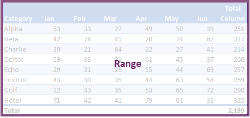
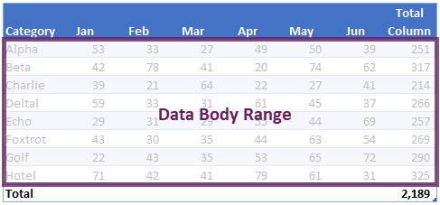
The data body range only includes the rows of data, it excludes the header and totals.
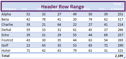
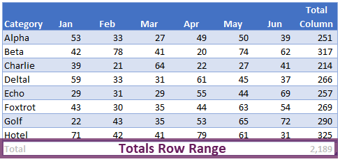
Header and total rows
The header row range is the top row of the table containing the column headers.
The totals row range, if displayed, includes calculations at the bottom of the table.
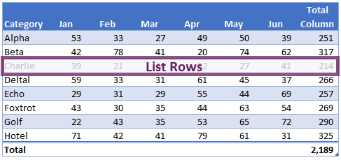
List columns and list rows
The individual columns are known as list columns.
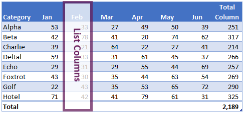
Each row is known as a list row.
The VBA code in this post details how to manage all these table objects.
Referencing the parts of a table
While you may be tempted to skip this section, I recommend you read it in full and work through the examples. Understanding Excel’s document object model is the key to reading and writing VBA code. Master this, and your ability to write your own VBA code will be much higher.
Many of the examples in this first section use the select method, this is to illustrate how to reference parts of the table. In reality, you would rarely use the select method.
Select the entire table
The following macro will select the whole table, including the totals and header rows.
Sub SelectTable()

ActiveSheet.ListObjects("myTable").Range.Select

End Sub
Select the data within a table
The DataBodyRange excludes the header and totals sections of the table.
Sub SelectTableData()

ActiveSheet.ListObjects("myTable").DataBodyRange.Select

End Sub
Get a value from an individual cell within a table
The following macro retrieves the table value from row 2, column 4, and displays it in a message box.
Sub GetValueFromTable()

MsgBox ActiveSheet.ListObjects("myTable").DataBodyRange(2, 4).value

End Sub
Select an entire column
The macro below shows how to select a column by its position, or by its name.
Sub SelectAnEntireColumn()

'Select column based on position
ActiveSheet.ListObjects("myTable").ListColumns(2).Range.Select

'Select column based on name
ActiveSheet.ListObjects("myTable").ListColumns("Category").Range.Select

End Sub
Select a column (data only)
This is similar to the macro above, but it uses the DataBodyRange to only select the data; it excludes the headers and totals.
Sub SelectColumnData()

'Select column data based on position
ActiveSheet.ListObjects("myTable").ListColumns(4).DataBodyRange.Select

'Select column data based on name
ActiveSheet.ListObjects("myTable").ListColumns("Category").DataBodyRange.Select

End Sub
Select a specific column header
This macro shows how to select the column header cell of the 5th column.
Sub SelectCellInHeader()

ActiveSheet.ListObjects("myTable").HeaderRowRange(5).Select

End Sub
Select a specific column within the totals section
This example demonstrates how to select the cell in the totals row of the 3rd column.
Sub SelectCellInTotal()

ActiveSheet.ListObjects("myTable").TotalsRowRange(3).Select

End Sub
Select an entire row of data
The macro below selects the 3rd row of data from the table.
NOTE – The header row is not included as a ListRow. Therefore, ListRows(3) is the 3rd row within the DataBodyRange, and not the 3rd row from the top of the table.
Sub SelectRowOfData()

ActiveSheet.ListObjects("myTable").ListRows(3).Range.Select

End Sub
Select the header row
The following macro selects the header section of the table.
Sub SelectHeaderSection()

ActiveSheet.ListObjects("myTable").HeaderRowRange.Select

End Sub
Select the totals row
To select the totals row of the table, use the following code.
Sub SelectTotalsSection()

ActiveSheet.ListObjects("myTable").TotalsRowRange.Select

End Sub
OK, now we know how to reference the parts of a table, it’s time to get into some more interesting examples.
Creating and converting tables
This section of macros focuses on creating and resizing tables.
Convert selection to a table
The macro below creates a table based on the currently selected region and names it as myTable. The range is referenced as Selection.CurrentRegion, but this can be substituted for any range object.
If you’re working along with the example file, this macro will trigger an error, as a table called myTable already exists in the workbook. A new table will still be created with a default name, but the VBA code will error at the renaming step.
Sub ConvertRangeToTable()

tableName As String
Dim tableRange As Range

Set tableName = "myTable"
Set tableRange = Selection.CurrentRegion
ActiveSheet.ListObjects.Add(SourceType:=xlSrcRange, _
    Source:=tableRange, _
    xlListObjectHasHeaders:=xlYes _
    ).Name = tableName

End Sub
Convert a table back to a range
This macro will convert a table back to a standard range.
Sub ConvertTableToRange()

ActiveSheet.ListObjects("myTable").Unlist

End Sub
NOTE – Unfortunately, when converting a table to a standard range, the table formatting is not removed. Therefore, the cells may still look like a table, even when they are not – that’s frustrating!!!
Resize the range of the table
To following macro resizes a table to cell A1 – J100.
Sub ResizeTableRange()

ActiveSheet.ListObjects("myTable").Resize Range("$A$1:$J$100")

End Sub
Table styles
There are many table formatting options, the most common of which are shown below.
Change the table style
Change the style of a table to an existing pre-defined style.
Sub ChangeTableStyle()

ActiveSheet.ListObjects("myTable").TableStyle = "TableStyleLight15"

End Sub
To apply different table styles, the easiest method is to use the macro recorder. The recorded VBA code will include the name of any styles you select.
Get the table style name
Use the following macro to get the name of the style already applied to a table.
Sub GetTableStyleName()

MsgBox ActiveSheet.ListObjects("myTable").TableStyle

End Sub
Apply a style to the first or last column
The first and last columns of a table can be formatted differently using the following macros.
Sub ColumnStyles()

'Apply special style to first column
ActiveSheet.ListObjects("myTable").ShowTableStyleFirstColumn = True

'Apply special style to last column
ActiveSheet.ListObjects("myTable").ShowTableStyleLastColumn = True

End Sub
Adding or removing stripes
By default, tables have banded rows, but there are other options for this, such as removing row banding or adding column banding.
Sub ChangeStripes()

'Apply column stripes
ActiveSheet.ListObjects("myTable").ShowTableStyleColumnStripes = True

'Remove row stripes
ActiveSheet.ListObjects("myTable").ShowTableStyleRowStripes = False

End Sub
Set the default table style
The following macro sets the default table style.
Sub SetDefaultTableStyle()

'Set default table style
ActiveWorkbook.DefaultTableStyle = "TableStyleMedium2"

End Sub
Looping through tables
The macros in this section loop through all the tables on the worksheet or workbook.
Loop through all tables on a worksheet
If we want to run a macro on every table of a worksheet, we must loop through the ListObjects collection.
Sub LoopThroughAllTablesWorksheet()

'Create variables to hold the worksheet and the table
Dim ws As Worksheet
Dim tbl As ListObject

Set ws = ActiveSheet
'Loop through each table in worksheet
For Each tbl In ws.ListObjects

    'Do something to the Table....

Next tbl

End Sub
In the code above, we have set the table to a variable, so we must refer to the table in the right way. In the section labeled ‘Do something to the table…, insert the action to be undertaken on each table, using tbl to reference the table.
For example, the following will change the table style of every table.
tbl.TableStyle = "TableStyleLight15"
Loop through all tables in a workbook
Rather than looping through a single worksheet, as shown above, the macro below loops through every table on every worksheet.
Sub LoopThroughAllTablesWorkbook()

'Create variables to hold the worksheet and the table
Dim ws As Worksheet
Dim tbl As ListObject

'Loop through each worksheet
For Each ws In ActiveWorkbook.Worksheets

    'Loop through each table in worksheet
    For Each tbl In ws.ListObjects

        'Do something to the Table....

    Next tbl

Next ws

End Sub
As noted in the section above, we must refer to the table using its variable. For example, the following will display the totals row for every table.
tbl.ShowTotals = True
Adding & removing rows and columns
The following macros add and remove rows, headers, and totals from a table.
Add columns into a table
The following macro adds a column to a table.
Sub AddColumnToTable()

'Add column at the end
ActiveSheet.ListObjects("myTable").ListColumns.Add

'Add column at position 2
ActiveSheet.ListObjects("myTable").ListColumns.Add Position:=2
End Sub
Add rows to the bottom of a table
The next macro will add a row to the bottom of a table
Sub AddRowsToTable()

'Add row at bottom
ActiveSheet.ListObjects("myTable").ListRows.Add

'Add row at the first row
ActiveSheet.ListObjects("myTable").ListRows.Add Position:=1
End Sub
Delete columns from a table
To delete a column, it is necessary to use either the column index number or the column header.
Sub DeleteColumnsFromTable()

'Delete column 2
ActiveSheet.ListObjects("myTable").ListColumns(2).Delete

'Delete a column by name
ActiveSheet.ListObjects("myTable").ListColumns("Feb").Delete
End Sub
Delete rows from a table
In the table structure, rows do not have names, and therefore can only be deleted by referring to the row number.
Sub DeleteRowsFromTable()

'Delete row 2
ActiveSheet.ListObjects("myTable").ListRows(2).Delete

'Delete multiple rows
ActiveSheet.ListObjects("myTable").Range.Rows("4:6").Delete
End Sub
Add total row to a table
The total row at the bottom of a table can be used for calculations.
Sub AddTotalRowToTable()

'Display total row with value in last column
ActiveSheet.ListObjects("myTable").ShowTotals = True

'Change the total for the "Total Column" to an average
ActiveSheet.ListObjects("myTable").ListColumns("TotalColumn").TotalsCalculation = _
    xlTotalsCalculationAverage

'Totals can be added by position, rather than name
ActiveSheet.ListObjects("myTable").ListColumns(2).TotalsCalculation = _
    xlTotalsCalculationAverage
End Sub
Types of totals calculation
xlTotalsCalculationNone
xlTotalsCalculationAverage
xlTotalsCalculationCount
xlTotalsCalculationCountNums
xlTotalsCalculationMax
xlTotalsCalculationMin
xlTotalsCalculationSum
xlTotalsCalculationStdDev
xlTotalsCalculationVar
Table header visability
Table headers can be turned on or off. The following will hide the headers.
Sub ChangeTableHeader()

ActiveSheet.ListObjects("myTable").ShowHeaders = False

End Sub
Remove auto filter
The auto filter can be hidden. Please note, the table header must be visible for this code to work.
Sub RemoveAutoFilter()

ActiveSheet.ListObjects("myTable").ShowAutoFilterDropDown = False

End Sub
I have a separate post about controlling auto filter settings – check it out here. Most of that post applies to tables too.
Other range techniques
Other existing VBA techniques for managing ranges can also be applied to tables.
Using the union operator
To select multiple ranges, we can use VBA’s union operator. Here is an example, it will select rows 4, 1, and 3.
Sub SelectMultipleRangesUnionOperator()

Union(ActiveSheet.ListObjects("myTable").ListRows(4).Range, _
    ActiveSheet.ListObjects("myTable").ListRows(1).Range, _
    ActiveSheet.ListObjects("myTable").ListRows(3).Range).Select

End Sub
Assign values from a variant array to a table row
To assign values to an entire row from a variant array, use code similar to the following:
Sub AssignValueToTableFromArray()

'Assing values to array (for illustration)
Dim myArray As Variant
myArray = Range("A2:D2")

'Assign values in array to the table
ActiveSheet.ListObjects("myTable").ListRows(2).Range.Value = myArray

End Sub
Reference parts of a table using the range object
Within VBA, a table can be referenced as if it were a standard range object.
Sub SelectTablePartsAsRange()

ActiveSheet.Range("myTable[Category]").Select

End Sub
Counting rows and columns
Often, it is useful to count the number of rows or columns. This is a good method to reference rows or columns which have been added.
Counting rows
To count the number of rows within the table, use the following macro.
Sub CountNumberOfRows()

Msgbox ActiveSheet.ListObjects("myTable").ListRows.Count

End Sub
Counting columns
The following macro will count the number of columns within the table.
Sub CountNumberOfColumns()

Msgbox ActiveSheet.ListObjects("myTable").ListColumns.Count

End Sub
Useful table techniques
The following are some other useful VBA codes for controlling tables.
Show the table data entry form
If a table starts at cell A1, there is a simple data entry form that can be displayed.
Sub ShowDataEntryForm()

'Only works if Table starts at Cell A1
ActiveSheet.ShowDataForm

End Sub
The following screenshot shows the data form for the example table.
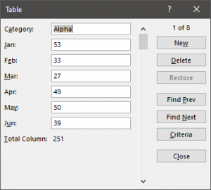
Check if a table exists
The following macro checks if a table already exists within a workbook. Change the tblName variable to adapt this to your requirements.
Sub CheckIfTableExists()

'Create variables to hold the worksheet and the table
Dim ws As Worksheet
Dim tbl As ListObject
Dim tblName As String
Dim tblExists As Boolean

tblName = "myTable"

'Loop through eac worksheet
For Each ws In ActiveWorkbook.Worksheets

    'Loop through each table in worksheet
    For Each tbl In ws.ListObjects

        If tbl.Name = tblName Then

            tblExists = True

        End If

    Next tbl

Next ws

If tblExists = True Then

    MsgBox "Table " & tblName & " exists."

Else

    MsgBox "Table " & tblName & " does not exists."

End If

End Sub
Find out if a table has been selected, if so which
The following macros find the name of the selected table.
Method 1
As you will see in the comments Jon Peltier had an easy approach to this, which has now become my preferred approach.
Sub SimulateActiveTable()

Dim ActiveTable As ListObject

On Error Resume Next
Set ActiveTable = ActiveCell.ListObject
On Error GoTo 0

'Confirm if a cell is in a Table
If ActiveTable Is Nothing Then
    MsgBox "Select table and try again"
Else
    MsgBox "The active cell is in a Table called: " & ActiveTable.Name
End If

End Sub
Method 2
This option, which was my original method, loops through each table on the worksheet and checks if they intersect with the active cell.
Sub SimulateActiveTable_Method2()

Dim ActiveTable As ListObject
Dim tbl As ListObject

'Loop through each table, check if table intersects with active cell
For Each tbl In ActiveSheet.ListObjects

    If Not Intersect(ActiveCell, tbl.Range) Is Nothing Then

        Set ActiveTable = tbl
        MsgBox "The active cell is in a Table called: " & ActiveTable.Name

    End If

Next tbl

'If no intersection then no tabl selected
If ActiveTable Is Nothing Then

    MsgBox "Select an Excel table and try again"

End If

End Sub
Conclusion
Wow! That was a lot of code examples.
There are over 30 VBA macros above, and even this does not cover everything, but hopefully covers 99% of your requirements. For your remaining requirements, you could try Microsoft’s VBA object reference library (https://docs.microsoft.com/en-us/office/vba/api/Excel.ListObject)

About the author
Hey, I’m Mark, and I run Excel Off The Grid.
My parents tell me that at the age of 7 I declared I was going to become a qualified accountant. I was either psychic or had no imagination, as that is exactly what happened. However, it wasn’t until I was 35 that my journey really began.
In 2015, I started a new job, for which I was regularly working after 10pm. As a result, I rarely saw my children during the week. So, I started searching for the secrets to automating Excel. I discovered that by building a small number of simple tools, I could combine them together in different ways to automate nearly all my regular tasks. This meant I could work less hours (and I got pay raises!). Today, I teach these techniques to other professionals in our training program so they too can spend less time at work (and more time with their children and doing the things they love).
Do you need help adapting this post to your needs?
I’m guessing the examples in this post don’t exactly match your situation. We all use Excel differently, so it’s impossible to write a post that will meet everybody’s needs. By taking the time to understand the techniques and principles in this post (and elsewhere on this site), you should be able to adapt it to your needs.
But, if you’re still struggling you should:
- Read other blogs, or watch YouTube videos on the same topic. You will benefit much more by discovering your own solutions.
- Ask the ‘Excel Ninja’ in your office. It’s amazing what things other people know.
- Ask a question in a forum like Mr Excel, or the Microsoft Answers Community. Remember, the people on these forums are generally giving their time for free. So take care to craft your question, make sure it’s clear and concise. List all the things you’ve tried, and provide screenshots, code segments and example workbooks.
- Use Excel Rescue, who are my consultancy partner. They help by providing solutions to smaller Excel problems.
What next?
Don’t go yet, there is plenty more to learn on Excel Off The Grid. Check out the latest posts:
Just copy the function below into a new module. I usually call this module ‘functions’
You can then call anywhere in your scripts `get_row_number(«dummy text», 1)
The integer ‘1’ will tell this to do a ctrl+f on column A. When it finds the first value it will return the row number of that value. Best used on columns that contain unique values otherwise it will reference the first value that it finds.
You might need to change the xlPart to xlWhole if you are going for an exact match.
You could also extend this function to pass in a boolean to look for whole or partial value and replace xlPart with the value passed in checkout https://gist.github.com/jaykilleen/892d0f0eed87b9f8e6b0 for other functions that I like to add into my ‘functions’ module.
  Function get_row_number(
      sheet As Worksheet,
      value As Variant,
      column As Integer
    ) As Integer

    get_row_number = Sheets(sheet.Name).Cells(1, column).EntireColumn.Find(
        What:=value,
        LookIn:=xlValues,
        LookAt:=xlPart,
        SearchOrder:=xlByColumns,
        SearchDirection:=xlNext,
        MatchCase:=False
      ).row

  End Function
Introduction to Range and Cells in VBA
When you look around in an Excel workbook, you will find that everything works around cells. A cell and a range of cells are where you store your data, and then everything starts.
To make the best of VBA, you need to learn how to use cells and ranges in your codes. For this, you need to have a solid understanding of Range objects. By using it, you can refer to cells in your codes in the following ways:
- A single cell.
- A range of cells
- A row or a column
- A three-dimensional range
The RANGE OBJECT is a part of Excel’s Object Hierarchy: Application ➜ Workbooks ➜ Worksheets ➜ Range and besides inside the worksheet. So if you are writing code to refer to the RANGE object it would be like this:
Application.Workbook(“Workbook-Name”).Worksheets(“Sheet-Name”).RangeBy referring to a cell or range of cells, you can do the following things:
- You can read the value from it.
- You can enter a value in it.
- And, you can make changes to the format.
To do all these things, you need to learn to refer to a cell or a range of cells, and in the next section of this tutorial, you will learn to refer to a cell using different ways.
To refer to a cell or a range of cells, you can use three different ways.
- Range Property
- Cells Property
- Offset Property
Well, which one is best out of these depends on your requirement, but it is worth learning all three so that you can choose which one is perfect for you.
So let’s get started.
Range Property
Range property is the most common and popular way to refer to a range in your VBA codes. With Range property, you simply need to refer to the cell address. Let me tell you the syntax.
expression.range(address)Here the expression is a variable representing a VBA object. So if you need to refer to the cell A1, the line of code you need to write would be:
Application.Workbook(“Book1”).Worksheets(“Sheet1”).Range(“A1”)The above code tells VBA that you are referring to cell A1 which is in the worksheet “Sheet1” and workbook ”Book1”.
Note: Whenever you type a cell address in the range object, make sure to wrap it in double quotation marks. But here’s one thing to understand. As you are using VBA in Excel there’s no need to use the word “Application”. So the code would be:
Workbook(“Book1”).Worksheets(“Sheet1”).Range(“A1”)And if you are in the Book1 there you can further trim down your code:
Worksheets(“Sheet1”).Range(“A1”)But, if you are already in the worksheet “Sheet1” then you can further trim down your code and can only use:
Range(“A1”)Now, let’s say if you want to refer to a full range of cells (i.e., multiple cells) you need to write the code in the following way:
Range("A1:A5")In the above code, you have referred to the range A1 to A5 which consists of the five cells. You can also refer to a named range using the range object. Let’s say you have named range with the name of “Sales Discount” to refer to this you can write a code like this:
Range("Sales Discount")If you want to refer to a non-continues range then you need to do something like this:
Range("A1:B5,D5:G10")And if you want to refer to an entire row or a column then you need to enter code like the below:
Range("1:1")
Range("A:A")
At this point, you have a clear understanding of how to refer to a cell and the range of cells. But to make it best with this you need to learn how to use this to do other things.
here we have a complete list of tutorials that you can use to learn to work with ranges and cells in VBA
- How to SET (Get and Change) Cell Value using a VBA Code
- How to Select a Range using VBA in Excel
- How to Create a Named Range using VBA (Static + Dynamic) in Excel
- How to Merge and Unmerge Cells in Excel using a VBA Code
- How to Check IF a Cell is Empty using VBA in Excel
- VBA ClearContents (from a Cell, Range, or Entire Worksheet)
- Excel VBA Font (Color, Size, Type, and Bold)
- How to AutoFit (Rows, Column, or the Entire Worksheet) using VBA
- How to use OFFSET Property with the Range Object or a Cell in VBA
- VBA Wrap Text (Cell, Range, and Entire Worksheet)
- How to Copy a CellRange to Another Sheet using VBA
- How to use Range/Cell as a Variable in VBA in Excel
- How to Find Last Rows, Column, and Cell using VBA in Excel
- How to use ActiveCell in VBA in Excel
- How to Refer to the UsedRange using VBA in Excel
- How to Change Row Height/Column Width using VBA in Excel
- How to SELECT ALL the Cells in a Worksheet using a VBA Code
- How to Insert a Row using VBA in Excel
- How to Insert a Column using VBA in Excel
1. Select and Activate a Cell
If you want to select a cell then you can use the Range. Select method. Let’s say if you want to select cell A5 then all you need to do is specify the range and then add “.Select” after that.
Range(“A1”).SelectThis code tells VBA to select cell A5 and if you want to select a range of cells then you just need to refer to that range and simply add “.Select” after that.
Range(“A1:A5”).SelectThere’s also another method that you can use to activate a cell.
Range(“A1”).ActivateHere you need to remember that you can activate only one cell at a time. Even if you specify a range with the “.Activate” method, it will select that range but the active cell will be the first cell of the range.
2. Enter a Value in a Cell
By using the range property you can enter a value in a cell or a range of cells. Let’s understand how it works using a simple example:
Range("A1").Value = "ExcelChamps"In the above example, you have specified the A1 as a range and after that, you have added “.Value” which tells VBA to access the value property of the cell.
The next thing you have is the equals sign and then the value which you want to enter (you need to use double quotation marks if you are entering a text value). For a number, the code would like this:
Range("A1").Value = 9988And if you want to enter a value into a range of cells, I mean multiple cells, then all you need to do is specify that range.
Range("A1:A5").Value = "ExcelChamps"And, here’s the code if you are referring to the non-continues range.
Range("A1:A5 , E2:E3").Value = "ExcelChamps"3. Copy and Paste a Cell/Range
With Range property, you can use the “.Copy” method to copy and cell and then paste it into a destination cell. Let’s say if you need to copy the cell A5 the code for this would be:
Range("A5").Copy When you run this code it will simply copy cell A5 but the next thing is to paste this copied cell to a destination cell. For this, you need to add the keyword destination after it and followed by the cell where you want to paste it. So if you want to copy cell A1 and then want to paste it to the cell E5, the code would be:
Range("A1").Copy Destination:=Range("E5")In the same way, if you are dealing with a range of multiple cells then the code would be like:
Range("A1:A5").Copy Destination:=Range("E5:E9")If you have copied a range of cells and then if you have mentioned one cell as the destination range, VBA will copy the entire copied range the starting from the cell you have specified as a destination.
Range("A1:A5").Copy Destination:=Range("B1")When you run the above code, VBA will copy range A1:A5 and will paste it to the B1:B5 even though you have mentioned only B1 as the destination range.
Tip: Just like the “.Copy” method you can use the “.Cut” method to cut a cell and then simply use a destination to paste it.
4. Use Font Property with Range Property
With the range property, you can access the font property of a cell which helps you to change all the font settings. There are a total of 18 different properties for the font which you can access. Let’s say if you want to make the text BOLD in cell A1, the code would be:
Range("A1").Font.Bold = TrueThis code tells VBA to access the BOLD property of the font which is inside the range A1 and you have set this property to TRUE. Now, let’s say you want to apply strikethrough to cell A1, this time the code would be:
As I said there are a total of 18 different properties you can use, so make sure to check out all of these to see which one is useful for you.
5. Clear Formatting from a Cell
By using the “.ClearFormats” method you can remove only the format from a cell or a range of cells. All you need to do is add “.ClearFormat” after specifying the range, like below:
Range("A1").ClearFormatsWhen you run the code above it clears all the formatting from cell A1 and if you want to do it for an entire range, you know what to do, Right?
Range("A1:A5").ClearFormatsNow the above code will simply remove the formatting from the range A1 to A5.
Cells Property
Apart from the RANGE property, you can use the “Cells” property to refer to a cell or a range of cells in your worksheet. In cell property, instead of using the cell reference, you need to enter the column number and row number of the cell.
expression.Cells(Row_Number, Column_Number)Here the expression is a VBA object and Row_Number is the row number of the cell and Column_Number is the column of the cell. So if you want to refer to the cell A5 you can use the code below code:
Cells(5,1)Now, this code tells VBA to refer to the cell which is at row number five and at column number one. As its syntax says you need to enter column number as address but the reality is you can also use the column alphabet if you want just by wrapping it in double quotation marks.
The below code will also refer to the cell A5:
Cells(5,"A")And to VBA to select it simply add “.Select” at the end.
Cells(5,1).SelectThe above code will select cell A5 which is in the 5th row and in the first column of the worksheet.
OFFSET Property
If you want to play well with ranges in VBA you need to know how to use the OFFSET property. It helps to refer to a cell that is a particular number of rows and columns away from another cell.
Let’s say your active cell is B5 right now and you want to navigate to the cell which is 3 columns right and 1 row down from B5, you can do this OFFSET. Below is the syntax which you need to use for the OFFSET:
expression.Offset (RowOffset, ColumnOffset)- RowOffset: In this argument, you need to specify a number that will tell VBA how many rows you want to navigate. A positive number defines a row downward and a negative number defines a row upward.
- ColumnOffset: In this argument, you need to specify a number that will tell VBA how many columns you want to navigate. A positive number defines a column to the right and a negative number defines a left.
Let’s write a simple code for example which we have discussed above.
- First, you need to define the range from where you want to navigate and so type the below code:

- After that, type “.Offset” and enter opening parentheses, just like below:

- Next, you need to enter the row number and then the column number where you want to navigate.

- In the end, you need to add “.Select” to tell VBA to select the cell where you want to navigate.


So when you run this code it will select the cell which is one row down and 3 columns right from cell B5.
Resize a Range using OFFSET
OFFSET not only allows you to navigate to a cell, but you can also resize the range further. Let’s continue the above example.
Range("B5").Offset(1, 3).SelectThe above code navigates you to cell E6, and now let’s say you need to select the range of cells that consists of the five columns and three rows from the E6. So what you need to do is after using OFFSET, use the resize property by adding “.Resize”.
Range("B5").Offset(1, 3).ResizeNow you need to enter the row size and column size. Type a starting parenthesis and enter the number to define the row size and then a number to define the column size.
Range("B5").Offset(1, 3).Resize(3,5)In the end, add “.Select” to tell VBA to select the range, and when you run this code, it will select the range.
Range("B5").Offset(1, 3).Resize(3, 5).SelectSo, when you run this code, it will select the range E6 to I8.
Range("A1").Font.Strikethrough = TrueMore Tutorials
- Count Rows using VBA in Excel
- Excel VBA Font (Color, Size, Type, and Bold)
- Excel VBA Hide and Unhide a Column or a Row
- Apply Borders on a Cell using VBA in Excel
- Find Last Row, Column, and Cell using VBA in Excel
- Insert a Row using VBA in Excel
- Merge Cells in Excel using a VBA Code
- Select a Range/Cell using VBA in Excel
- SELECT ALL the Cells in a Worksheet using a VBA Code
- ActiveCell in VBA in Excel
- Special Cells Method in VBA in Excel
- UsedRange Property in VBA in Excel
- VBA AutoFit (Rows, Column, or the Entire Worksheet)
- VBA ClearContents (from a Cell, Range, or Entire Worksheet)
- VBA Copy Range to Another Sheet + Workbook
- VBA Enter Value in a Cell (Set, Get and Change)
- VBA Insert Column (Single and Multiple)
- VBA Named Range | (Static + from Selection + Dynamic)
- VBA Range Offset
- VBA Sort Range | (Descending, Multiple Columns, Sort Orientation
- VBA Wrap Text (Cell, Range, and Entire Worksheet)
- VBA Check IF a Cell is Empty + Multiple Cells
⇠ Back to What is VBA in Excel
Helpful Links – Developer Tab – Visual Basic Editor – Run a Macro – Personal Macro Workbook – Excel Macro Recorder – VBA Interview Questions – VBA Codes