
Bottom Line: Learn 4 different techniques for creating a list of numbers in Excel. These include both static and dynamic lists that change when items are added or deleted from the list.
Skill Level: Beginner
Watch the Tutorial
Download the Excel File
You can download the worksheet that I use in the video here:
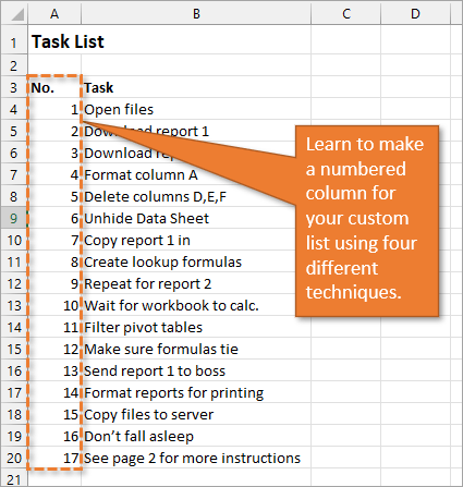
If you have a list of items in Excel and you’d like to insert a column that numbers the items, there are several ways to accomplish this. Let’s look at four of those ways.
1. Create a Static List Using Auto-Fill
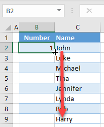
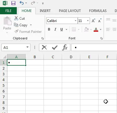
The first way to number a list is really easy. Start by filling in the first two numbers of your list, select those two numbers, and then hover over the bottom right corner of your selection until your cursor turns into a plus symbol. This is the fill handle.
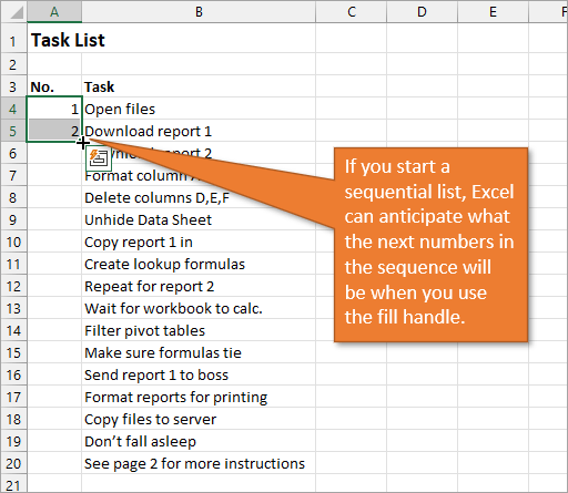
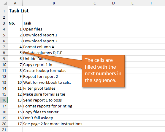
When you double-click on that fill handle (or drag it down to the end of your list), Excel will fill in the blanks with the next numbers in the sequence.
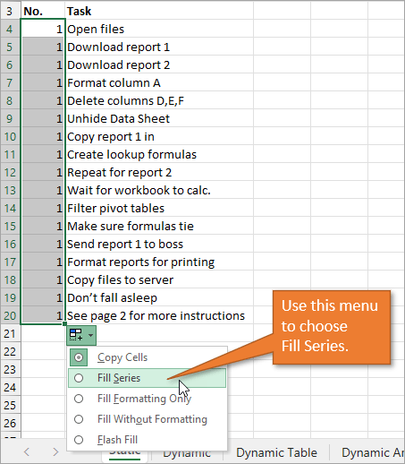
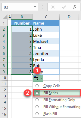
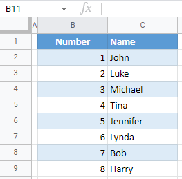
An alternate way to create this same numbered list is to type a 1 in the first cell and then double-click the fill handle. Because Excel doesn’t have a second number to identify a sequence or pattern, it will fill down the columns with 1s. But you will notice that a menu is available at the end of your column, and from that menu, you can select the option to Fill Series. This will change the 1s to a sequential list of numbers.
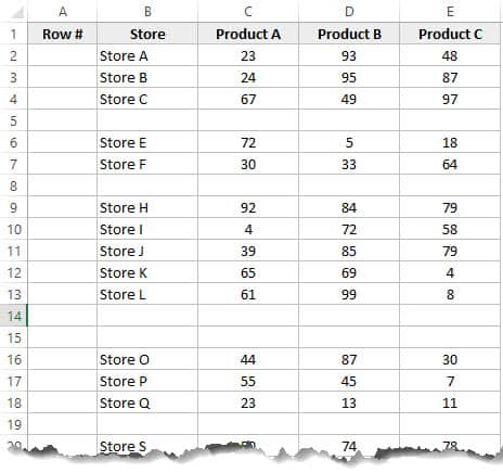
The numbered column we’ve created in both instances is static. This means it doesn’t change when you make additions or deletions to the corresponding list of items. For example, if I insert a new row in order to add another task, there is a break in the numbered column as well, and I would have to repeat the same steps to correct the list.
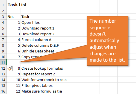
So, unless we want the numbers to always remain as they are, a better option would be to create a dynamic list.
2. Create a Dynamic List Using a Formula
We can use formulas to create a dynamic list where the numbers update when we add or delete rows from the list.
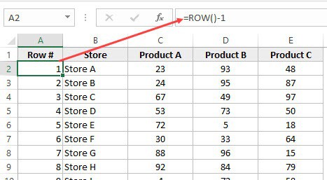
To use a formula for creating a dynamic number list, we can use the ROW function. The ROW function returns the row number of a cell. If we don’t specify a cell for ROW, it just returns the current row number of whatever is selected.
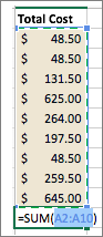
In our example, the first cell in our list doesn’t start on Row 1. It starts on Row 4. But we don’t want our list to start at 4; we want it to start at 1. To subtract the extra 3, our formula will include a minus sign and then the ROW function again, but this time pointed to the cell above our formula (which is in Row 3).
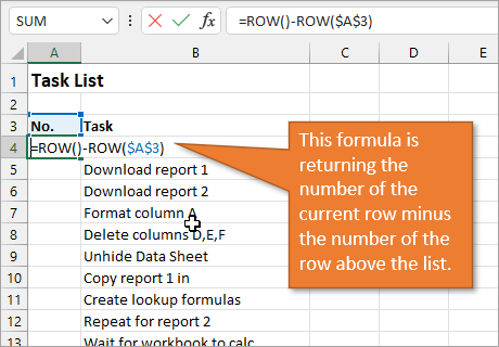
We use the absolute values (dollar signs) in our cell selection because we don’t want that number to change as we copy the formula down the list. In other words, we always want to subtract 3 from the row number to give us our list number.
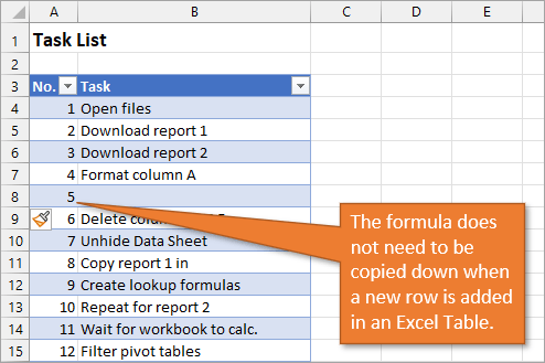
When we copy down the formula, we have a numbered list that will adjust when we add or delete rows. However, when adding a row, we will have to copy the formula into the newly inserted cell.
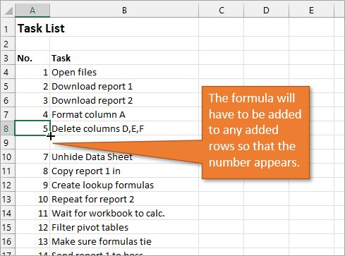
This additional step of copying the formula into new rows can be avoided if we use Excel Tables.
3. Create a Dynamic List Using a Formula in an Excel Table
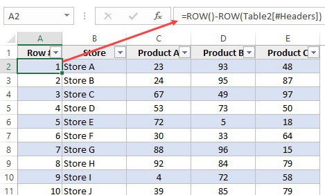
If we write the same formula but we use an Excel table, the only difference we will make in the formula is that we reference the column header instead of the absolute cell value.
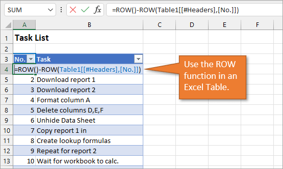
Because we are using an Excel Table, the formula automatically fills down to the other rows. When we add a row to the table, the formula will automatically populate in the new cell.
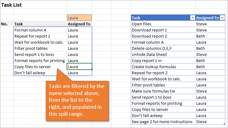
4. Create a Dynamic List Using Dynamic Array Formulas
Below, I have a table that is populated using Dynamic Array Formulas. The FILTER formula spills a range of results based on whatever name is selected in the orange cell.
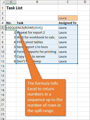
The Dynamic Array formula we will use is SEQUENCE. This will return a sequence for the number of rows we identify in the formula. To tell Excel how many rows there are, we will use the ROW function as the argument for sequence. The argument for ROW is just the spill range. The way to notate the spill range is to simply place a hashtag after the name of the first cell in the range. So our formula looks like this:
=SEQUENCE(ROWS(B5#))
Once we complete our formula and hit Enter, the list will be numbered.
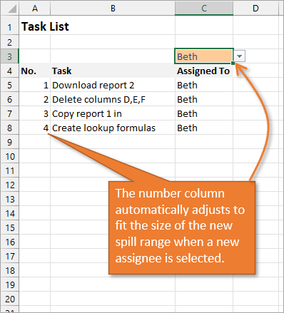
With this formula in place, if the size of the range changes when a new name is selected, the numbered column for the list will automatically adjust as well.
Bonus Tip: Formatting Your Numbered List
If you want to add periods or other punctuation to your numbered list:
- Select the entire list and right-click to choose Format Cells. Or use the keyboard shortcut Ctrl + 1.
- Choose the Custom option on the Number tab.
- Then in the Type field, type in the number 0 with whatever punctuation you would like to surround your number.
Here, I’ve just added a period.
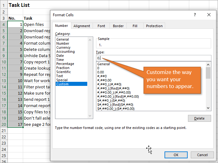
When you hit OK, you will have formatted the entire selection.
Related Posts
Here are a few similar posts that may interest you.
- Excel Tables Tutorial Video – Beginners Guide for Windows & Mac
- New Excel Features: Dynamic Array Formulas & Spill Ranges
- How to Prevent Excel from Freezing or Taking A Long Time when Deleting Rows
Conclusion
I hope these four ways to create ordered lists are helpful for you. If you have questions or feedback, I would love to hear them in the comments. Have a great week!
Updated: 02/01/2021 by

A bulleted and numbered list is an available feature in Microsoft Excel, but not as commonly used as in word processing documents or presentation slides. By default, the bulleted and numbered lists option is hidden in Excel and must be added to the Ribbon. Additionally, a bulleted and numbered list cannot be added to a cell in Excel. A text box must be created, and then a bulleted or numbered list is added to that text box.
Create a bulleted or numbered list in Excel
Add bulleted and numbered list option to the Ribbon
- Open Microsoft Excel.
- Click the File tab in the Ribbon.
- Click Options in the left navigation menu.
- In the Excel Options window, click Customize Ribbon in the left navigation menu.
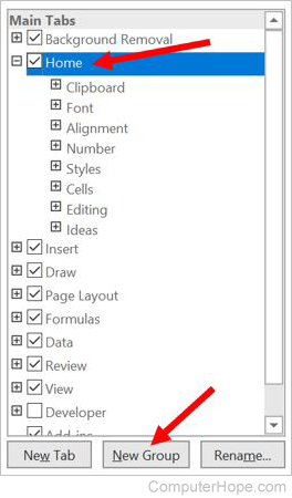
- On the right side of the Excel Options window, click the Home entry in the Main Tabs box.
- Click the New Group button below the Main Tabs box.
- A new group is added to the Home group. Click the New Group (Custom) entry, and click the Rename button.
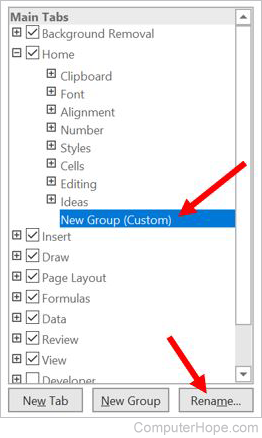
- Enter a new name, like Bullets or Bullet Lists, for the group.
- On the left side of the Excel Options window, click the Choose commands from drop-down list and select All Commands.
- In the list below, scroll down and find the Bullets and Numbering option. Click that entry and drag it to the new group you created on the right.
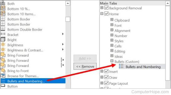
- Click the OK button to create the new group on the Home tab in the Ribbon, with the Bullets and Numbering option in it. The new group and option is found on the Home tab, on the far right side.
Add a text box to a worksheet
- Click the Insert tab in the Ribbon.
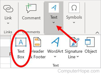
- On the Insert tab, click the Text option on the far right side, and select the Text Box option.
- In the worksheet, press and hold the left mouse button where you want to create the text box. Drag the mouse down and to the right, creating the text box with the desired size.
Add bulleted or numbered list to the text box
- Click in the text box you added to the worksheet.
- Click the Home tab in the Ribbon.
- Click the Bullets and Numbering option in the new group you created. The new group is on the far right side of the Home tab.
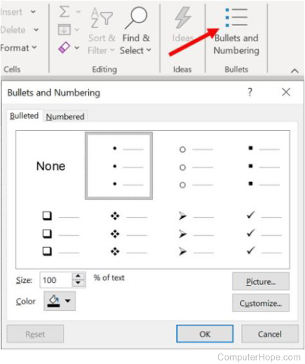
- In the Bullets and Numbering window, select the type of bulleted or numbered list you want to add to the text box and click OK.
- Type the text for each bullet point in the text box, pressing Enter to create the next bullet point.
- After entering the text for all desired bullet points, you can move the text box to any location in the worksheet. You can also resize the text box to better fit the bulleted or numbered list, if necessary.
Содержание
- How to Make a List of Numbers in Excel & Google Sheets
- AutoFill Numbers
- Double-Click the Fill Handle
- Fill Command
- AutoFill Numbers in Google Sheets
- How to create a bulleted or numbered list in Microsoft Excel
- Create a bulleted or numbered list in Excel
- Add bulleted and numbered list option to the Ribbon
- Add a text box to a worksheet
- Add bulleted or numbered list to the text box
- Automatically number rows
- What do you want to do?
- Fill a column with a series of numbers
- Use the ROW function to number rows
- Display or hide the fill handle
- Add a list of numbers in a column
- Excel: Listing Numbers In Between 2 Numbers
- 3 Answers 3
How to Make a List of Numbers in Excel & Google Sheets
This tutorial demonstrates how to make a list of numbers in Excel and Google Sheets.
AutoFill Numbers
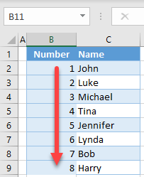
Say you have data in two columns in Excel. In Column C, there are names, while in Column B, you want to assign a number to each name, i.e., make a list of numbers in Column B.
Double-Click the Fill Handle
You can use AutoFill, by double-clicking, to populate cells based on the adjacent columns (non-blank columns to the left and right of the selected column). In this case, numbers are populated through Row 9.
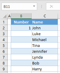
- Enter 1 in cell B2. This is the initial data for Excel to recognize the pattern for AutoFill functionality.
- Position the cursor in the bottom-right corner of cell B2, and double-click the fill handle (the little black cross that appears).
- Click on AutoFill options and select Fill Series. Consecutive numbers are automatically populated through cell B9.
Fill Command
The above example could also be achieved using the Fill command on the Ribbon.
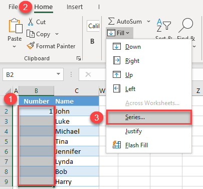
- Select the range of cells – including the initial value – where you want numbers populated (B2:B9). Then in the Ribbon, go to Home > Fill > Series.
- In the pop-up screen, leave the default values: The column should be populated, and the Step value (increment) is 1. Press OK.
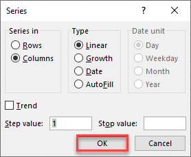
You get the same output: Numbers 1–8 fill cells B2:B9.
AutoFill Numbers in Google Sheets
You can also autofill numbers by double-clicking the fill handle (or just dragging it) in Google Sheets. Unlike in Excel, you need at least two numbers in Google Sheets to be able to recognize a pattern.
- Enter 1 in cell B2, and 2 in cell B3. This is the initial data for Google Sheets to recognize the pattern for AutoFill functionality.
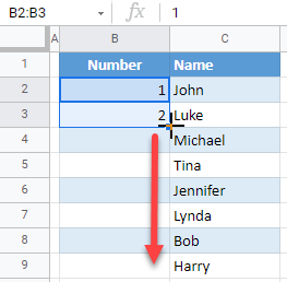
- Select cells B2 and B3, position the cursor in the bottom-right corner of cell B3, and double-click the fill handle.
As a result, a list of consecutive number is filled in Column B.
Источник
How to create a bulleted or numbered list in Microsoft Excel
A bulleted and numbered list is an available feature in Microsoft Excel, but not as commonly used as in word processing documents or presentation slides. By default, the bulleted and numbered lists option is hidden in Excel and must be added to the Ribbon. Additionally, a bulleted and numbered list cannot be added to a cell in Excel. A text box must be created, and then a bulleted or numbered list is added to that text box.
Create a bulleted or numbered list in Excel
Add bulleted and numbered list option to the Ribbon
- Open Microsoft Excel.
- Click the File tab in the Ribbon.
- Click Options in the left navigation menu.
- In the Excel Options window, click Customize Ribbon in the left navigation menu.
- On the right side of the Excel Options window, click the Home entry in the Main Tabs box.
- Click the New Group button below the Main Tabs box.
- A new group is added to the Home group. Click the New Group (Custom) entry, and click the Rename button.
- Enter a new name, like Bullets or Bullet Lists, for the group.
- On the left side of the Excel Options window, click the Choose commands from drop-down list and select All Commands.
- In the list below, scroll down and find the Bullets and Numbering option. Click that entry and drag it to the new group you created on the right.
- Click the OK button to create the new group on the Home tab in the Ribbon, with the Bullets and Numbering option in it. The new group and option is found on the Home tab, on the far right side.
Add a text box to a worksheet
- Click the Insert tab in the Ribbon.
- On the Insert tab, click the Text option on the far right side, and select the Text Box option.
- In the worksheet, press and hold the left mouse button where you want to create the text box. Drag the mouse down and to the right, creating the text box with the desired size.
Add bulleted or numbered list to the text box
- Click in the text box you added to the worksheet.
- Click the Home tab in the Ribbon.
- Click the Bullets and Numbering option in the new group you created. The new group is on the far right side of the Home tab.
- In the Bullets and Numbering window, select the type of bulleted or numbered list you want to add to the text box and click OK.
- Type the text for each bullet point in the text box, pressing Enter to create the next bullet point.
- After entering the text for all desired bullet points, you can move the text box to any location in the worksheet. You can also resize the text box to better fit the bulleted or numbered list, if necessary.
Источник
Automatically number rows
Unlike other Microsoft 365 programs, Excel does not provide a button to number data automatically. But, you can easily add sequential numbers to rows of data by dragging the fill handle to fill a column with a series of numbers or by using the ROW function.
Tip: If you are looking for a more advanced auto-numbering system for your data, and Access is installed on your computer, you can import the Excel data to an Access database. In an Access database, you can create a field that automatically generates a unique number when you enter a new record in a table.

What do you want to do?
Fill a column with a series of numbers
Select the first cell in the range that you want to fill.
Type the starting value for the series.
Type a value in the next cell to establish a pattern.
Tip: For example, if you want the series 1, 2, 3, 4, 5. type 1 and 2 in the first two cells. If you want the series 2, 4, 6, 8. type 2 and 4.
Select the cells that contain the starting values.
Note: In Excel 2013 and later, the Quick Analysis button is displayed by default when you select more than one cell containing data. You can ignore the button to complete this procedure.
Drag the fill handle  across the range that you want to fill.
Note: As you drag the fill handle across each cell, Excel displays a preview of the value. If you want a different pattern, drag the fill handle by holding down the right-click button, and then choose a pattern.
To fill in increasing order, drag down or to the right. To fill in decreasing order, drag up or to the left.
Tip: If you do not see the fill handle, you may have to display it first. For more information, see Display or hide the fill handle.
Note: These numbers are not automatically updated when you add, move, or remove rows. You can manually update the sequential numbering by selecting two numbers that are in the right sequence, and then dragging the fill handle to the end of the numbered range.
Use the ROW function to number rows
In the first cell of the range that you want to number, type =ROW(A1).
The ROW function returns the number of the row that you reference. For example, =ROW(A1) returns the number 1.
Drag the fill handle across the range that you want to fill.
Tip: If you do not see the fill handle, you may have to display it first. For more information, see Display or hide the fill handle.
These numbers are updated when you sort them with your data. The sequence may be interrupted if you add, move, or delete rows. You can manually update the numbering by selecting two numbers that are in the right sequence, and then dragging the fill handle to the end of the numbered range.
If you are using the ROW function, and you want the numbers to be inserted automatically as you add new rows of data, turn that range of data into an Excel table. All rows that are added at the end of the table are numbered in sequence. For more information, see Create or delete an Excel table in a worksheet.
To enter specific sequential number codes, such as purchase order numbers, you can use the ROW function together with the TEXT function. For example, to start a numbered list by using 000-001, you enter the formula =TEXT(ROW(A1),»000-000″) in the first cell of the range that you want to number, and then drag the fill handle to the end of the range.
Display or hide the fill handle
The fill handle displays by default, but you can turn it on or off.
In Excel 2010 and later, click the File tab, and then click Options.
In Excel 2007, click the Microsoft Office Button  , and then click Excel Options.
In the Advanced category, under Editing options, select or clear the Enable fill handle and cell drag-and-drop check box to display or hide the fill handle.
Note: To help prevent replacing existing data when you drag the fill handle, ensure the Alert before overwriting cells check box is selected. If you do not want Excel to display a message about overwriting cells, you can clear this check box.
Источник
Add a list of numbers in a column
To quickly get a total instead of typing each number into a calculator.
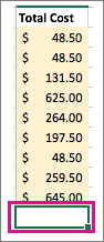
Click the first empty cell below a column of numbers.
Do one of the following:
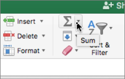
Excel 2016 for Mac: : On the Home tab, click AutoSum.
Excel for Mac 2011: On the Standard toolbar, click AutoSum.
Tip: If the blue border does not contain all of the numbers that you want to add, adjust it by dragging the sizing handles on each corner of the border.
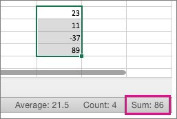
If you want a quick total that doesn’t have to appear on the sheet, select all the numbers in the list, and then look at the status bar at the bottom of the workbook window.
You can quickly insert the AutoSum formula by typing the  + SHIFT + T keyboard shortcut.
Источник
Excel: Listing Numbers In Between 2 Numbers
I was wondering if anyone knew of a formula to list all the numbers between 2 values, so for example if cell F2 had 12 in it and G2 had 17 in it I’d like a formula that would show 13,14,15,16 In cell H2.
3 Answers 3
This cannot be done with an Excel worksheet function. You will need VBA for that. It can be done with a user-defined function (UDF).
The following code needs to be stored in a code Module. You need to right-click the sheet tab, select View Code. This will open the Visual Basic Editor. Click Insert > Module and then paste the following code:
Now you can use a formula like =InBetween(F2,G2) to produce the result you describe.
You need to save the file as a macro-enabled workbook with the XLSM extension. See screenshot for code and user defined function in action.

Just because @teylyn said it couldn’t be done with a formula — here is a formula based solution:
First you need to create the full list of numbers that you are likely to need as a string, this could be in another cell or my preference would be to create a named range.
So create a new named range called rng and in the Refers to text box add the following formula:
For this solution to work you have to know the full range upfront, also note the leading and trailing comma.
Then enter the following formula into cell H2:
To same the tedium of creating the number range string I used the following Powershell code to create and copy it to the clipboard:
Just change the 20 in the above code for whatever range you require.
Источник
Excel for Microsoft 365 for Mac Excel 2021 for Mac Excel 2019 for Mac Excel 2016 for Mac Excel for Mac 2011 More…Less
Why?
To quickly get a total instead of typing each number into a calculator.
How?
-
Click the first empty cell below a column of numbers.

-
Do one of the following:
-
Excel 2016 for Mac: : On the Home tab, click AutoSum.
-
Excel for Mac 2011: On the Standard toolbar, click AutoSum.
Tip: If the blue border does not contain all of the numbers that you want to add, adjust it by dragging the sizing handles on each corner of the border.
-
-
Press RETURN .
Tips:
-
If you want a quick total that doesn’t have to appear on the sheet, select all the numbers in the list, and then look at the status bar at the bottom of the workbook window.
-
You can quickly insert the AutoSum formula by typing the
+ SHIFT + T keyboard shortcut.
Need more help?
Want more options?
Explore subscription benefits, browse training courses, learn how to secure your device, and more.
Communities help you ask and answer questions, give feedback, and hear from experts with rich knowledge.
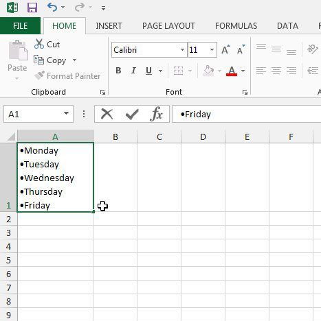
В Microsoft Word есть замечательная команда в меню Формат — Список (Format — Bullets and Numbering), позволяющая быстро превратить набор абзацев в маркированный или нумерованный список. Быстро, удобно, наглядно, не надо следить за нумерацией. В Excel такой функции нет, но можно попробовать ее имитировать с помощью несложных формул и форматирования.
Маркированный список
Выделите ячейки с данными для списка, щелкните по ним правой кнопкой мыши и выберите Формат ячеек (Format Cells), вкладка Число (Number), далее — Все форматы (Custom). Затем в поле Тип введите следующую маску пользовательского формата:

Для ввода жирной точки можно воспользоваться сочетанием клавиш Alt+0149 (удерживая Alt, набрать 0149 на цифровой клавиатуре).
Нумерованный список
Выделите пустую ячейку слева от начала списка (на рисунке это С1) и введите в нее следующую формулу:
=ЕСЛИ(ЕПУСТО(D1);»»;СЧЁТЗ($D$1:D1))
=IF(ISBLANK(D1);»»;COUNTA($D$1:D1))
Затем скопируйте формулу на весь столбец. У Вас должно получиться примерно следующее:

Фактически, формула в столбце С проверяет содержимое соседней справа ячейки (функции ЕСЛИ и ЕПУСТО). Если соседняя ячейка пустая, то не выводим ничего (пустые кавычки). Если не пустая, то выводим количество непустых ячеек (функция СЧЁТЗ) от начала списка до текущей ячейки, то есть порядковый номер.
How do I create a numbered list in one cell in Excel?
Select a blank cell that you want to create a bulleted list, and hold Alt key, press 0149 in the number tab, and then a bullet is inserted. 3. Repeat above steps to create the values one by one.
How do I create a list in an Excel cell?
Create a drop-down list
- Select the cells that you want to contain the lists.
- On the ribbon, click DATA > Data Validation.
- In the dialog, set Allow to List.
- Click in Source, type the text or numbers (separated by commas, for a comma-delimited list) that you want in your drop-down list, and click OK.
How do I insert numbered bullets in Excel?
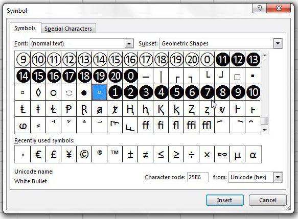
Select a blank cell, and then on the Insert tab, click Symbol. At the bottom of the dialog box, type 2022 in the Character code box. Then click Insert, and Close. If you need another bullet on a new line underneath, type ALT+ENTER and repeat the process.
How do I insert a list of numbers in Excel?
Add a list of numbers in a column
- Click the first empty cell below a column of numbers.
- Do one of the following: Excel 2016 for Mac: : On the Home tab, click AutoSum. Excel for Mac 2011: On the Standard toolbar, click AutoSum.
- Press RETURN .
How do I get a list of numbers in sheets?
Use autofill to complete a series
- On your computer, open a spreadsheet in Google Sheets.
- In a column or row, enter text, numbers, or dates in at least two cells next to each other.
- Highlight the cells. You’ll see a small blue box in the lower right corner.
- Drag the blue box any number of cells down or across.
How do I create a sequential formula in Excel?
What is the first character you put while inserting a formula?
All formulas begin with an equal sign (=). You can create a simple formula by using constant and calculation operator. For example, the formula =5+2*3, multiplies two numbers and then adds a number to the result.
How do I create a sequence in Excel 2013?
Excel SEQUENCE Function
- rows – Number of rows to return.
- columns – [optional] Number of columns to return.
- start – [optional] Starting value (defaults to 1).
- step – [optional] Increment between each value (defaults to 1).
How do you create a number range in Excel?
How to Create Named Ranges in Excel
- Select the range for which you want to create a Named Range in Excel.
- Go to Formulas –> Define Name.
- In the New Name dialogue box, type the Name you wish to assign to the selected data range.
- Click OK.
How do I create a sequence in Excel 2016?
Here’s a simple guide. First, enter all contents you want to generate the sequence numbers. Then, enter the formula “=Row()-1 ” in the cell “A2”, and press Enter in keyboard, then you get the result of row 2. Next, select “A2” and move the mouse to the bottom right corner of it, a small black cross appears.
How do you continue numbering in Excel?
Type 1 into a cell that you want to start the numbering, then drag the autofill handle at the right-down corner of the cell to the cells you want to number, and click the fill options to expand the option, and check Fill Series, then the cells are numbered.
How do you create a number sequence in excel without dragging?
Quickly Fill Numbers in Cells without Dragging
- Enter 1 in cell A1.
- Go to Home –> Editing –> Fill –> Series.
- In the Series dialogue box, make the following selections: Series in: Columns. Type: Linear. Step Value: 1. Stop Value: 1000.
- Click OK.
Why is Excel not auto numbering?
To fix this you have to go into Options / Edit tab and enable “Allow cell drag and drop”. Now you should be able to see the cursor change when you hover over the bottom right corner, and you’ll need to right-click drag in order to fill the series. Hope that helps!
How rows are numbered in MS Excel?
“Rows” run “horizontally” across the “worksheet & ranges” from “1 to 1048576”. A row is generally identified by the number that is on the “left side” of the “row“, from where the “row originates”. “Columns” run “vertically” “downward” across the “worksheet & ranges” from “A to XFD” – “1 to 16384”.
How many cell in MS Excel?
How many sheets, rows, and columns can a spreadsheet have?
| Version | Rows | Cells |
|---|---|---|
| Excel 2016 | 1,048,576 | 17,179,869,184 |
| Excel 2013 | 1,048,576 | 17,179,869,184 |
| Excel 2007 | 1,048,576 | 17,179,869,184 |
| Excel 2003 and earlier | 65,536 | 16,777,216 |
•
Jun 30, 2019
What is ROW () in Excel?
The Excel ROW function returns the row number for a reference. When no reference is provided, ROW returns the row number of the cell which contains the formula. Get the row number of a reference. A number representing the row.
What is the shortcut key for serial number in Excel?
How do you write a short serial number?
Abbreviation for Serial Number:
S. No.
How do I automatically number rows in numbers?
How do I autofill in Excel using keyboard?
Simply do the following: Select the cell with the formula and the adjacent cells you want to fill. Click Home > Fill, and choose either Down, Right, Up, or Left. Keyboard shortcut: You can also press Ctrl+D to fill the formula down in a column, or Ctrl+R to fill the formula to the right in a row.
How can I create a formula in Excel?
How do I turn on autofill in Excel?
Turn automatic completion of cell entries on or off
- Click File > Options.
- Click Advanced, and then under Editing options, select or clear the Enable AutoComplete for cell values check box to turn this option on or off.
See all How-To Articles
This tutorial demonstrates how to make a list of numbers in Excel and Google Sheets.
AutoFill Numbers
Say you have data in two columns in Excel. In Column C, there are names, while in Column B, you want to assign a number to each name, i.e., make a list of numbers in Column B.
Double-Click the Fill Handle
You can use AutoFill, by double-clicking, to populate cells based on the adjacent columns (non-blank columns to the left and right of the selected column). In this case, numbers are populated through Row 9.
- Enter 1 in cell B2. This is the initial data for Excel to recognize the pattern for AutoFill functionality.
- Position the cursor in the bottom-right corner of cell B2, and double-click the fill handle (the little black cross that appears).
- Click on AutoFill options and select Fill Series. Consecutive numbers are automatically populated through cell B9.
Fill Command
The above example could also be achieved using the Fill command on the Ribbon.
- Select the range of cells – including the initial value – where you want numbers populated (B2:B9). Then in the Ribbon, go to Home > Fill > Series.
- In the pop-up screen, leave the default values: The column should be populated, and the Step value (increment) is 1. Press OK.
You get the same output: Numbers 1–8 fill cells B2:B9.
AutoFill Numbers in Google Sheets
You can also autofill numbers by double-clicking the fill handle (or just dragging it) in Google Sheets. Unlike in Excel, you need at least two numbers in Google Sheets to be able to recognize a pattern.
- Enter 1 in cell B2, and 2 in cell B3. This is the initial data for Google Sheets to recognize the pattern for AutoFill functionality.
- Select cells B2 and B3, position the cursor in the bottom-right corner of cell B3, and double-click the fill handle.
As a result, a list of consecutive number is filled in Column B.
Microsoft Excel’s default layout of cells in rows and columns is a great place to start when you’re organizing data. But you might be wondering how to add a bulleted or numbered list in Excel cell objects if you need another level of organization.
How to Add Bullets in Excel 2013
- Click inside the cell where you want to add bullets.
- Hold down the Alt key, then press 0, then 1, then 4, then 9.
- Enter the information for the first bullet, then hold down the Alt key on your keyboard and press Enter to move to the next line within that cell.
- Repeat steps 2 and 3 for each additional bullet item that you wish to add in Excel.
Our guide continues below with additional information on adding a bulleted or numbered list in Excel cell, including pictures of these steps.
Adding bullets in Excel is something that might seem like an obvious feature to include in the program but, if you are reading this article, you have probably found that it is not the case.
Microsoft Word and Powerpoint make it very easy to create bulleted or numbered lists, and you can also learn how to put a bullet point on Google Slides. This can happen so easily that you might not even be trying to create a list. But Excel 2013 does not offer a similar automatic list option, nor is there a way on the ribbon for you to enter one manually.
Fortunately, you can add a bullet before a list item using a keyboard shortcut. You can even elect to add multiple bulleted items into a single cell with the help of a line break keyboard shortcut.
Our guide below will show you how.
How to Make a Multi-Item Bullet Lists in a Single Cell in Excel 2013 (guide with Pictures)
The steps in this article are going to show you how to create a bulleted list of two or more items inside a single cell of an Excel worksheet.
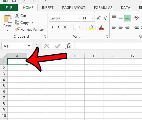
Step 1: Open a worksheet in Excel 2013.
Step 2: Click inside the cell where you would like to insert the bulleted list.
You can resize the row or resize the column now if you want, or you can do it later. It’s up to you.
Step 3: Hold down the Alt key on your keyboard, then press 0, then 1, then 4, then 9.
This should insert a bullet into the cell.
Step 4: You can then type the information that you want to include as the first bulleted item.
Once you have reached the end of the first line, hold down the Alt key on the keyboard, then press Enter. You can continue adding bullets by pressing Alt +0149 and adding line breaks by pressing Alt + Enter.
Rather than bullets you could also just type a number followed by a period, then use the Alt + Enter line break option for a numbered list in an Excel cell.
You can use different items as bullets by selecting them from the Symbols menu on the Insert tab as well, clicking a symbol on the menu, then clicking the Insert button to insert it into the cell.
For example, if you wanted to use a numbered list in Excel cell formatting, then you could use these numbers instead of the bullets that we discussed above.
You can force Excel 2013 to automatically resize rows or columns to fit the size of their data by reading this article – https://www.solveyourtech.com/automatically-resize-row-height-excel-2013/ . This can save some frustration if your row or column sizing is acting difficultly.
Additional Sources

Matthew Burleigh has been writing tech tutorials since 2008. His writing has appeared on dozens of different websites and been read over 50 million times.
After receiving his Bachelor’s and Master’s degrees in Computer Science he spent several years working in IT management for small businesses. However, he now works full time writing content online and creating websites.
His main writing topics include iPhones, Microsoft Office, Google Apps, Android, and Photoshop, but he has also written about many other tech topics as well.
Read his full bio here.
Watch Video – 7 Quick and Easy Ways to Number Rows in Excel
When working with Excel, there are some small tasks that need to be done quite often. Knowing the ‘right way’ can save you a great deal of time.
One such simple (yet often needed) task is to number the rows of a dataset in Excel (also called the serial numbers in a dataset).
Now if you’re thinking that one of the ways is to simply enter these serial number manually, well – you’re right!
But that’s not the best way to do it.
Imagine having hundreds or thousands of rows for which you need to enter the row number. It would be tedious – and completely unnecessary.
There are many ways to number rows in Excel, and in this tutorial, I am going to share some of the ways that I recommend and often use.
Of course, there would be more, and I will be waiting – with a coffee – in the comments area to hear from you about it.
How to Number Rows in Excel
The best way to number the rows in Excel would depend on the kind of data set that you have.
For example, you may have a continuous data set that starts from row 1, or a dataset that start from a different row. Or, you might have a dataset that has a few blank rows in it, and you only want to number the rows that are filled.
You can choose any one of the methods that work based on your dataset.
1] Using Fill Handle
Fill handle identifies a pattern from a few filled cells and can easily be used to quickly fill the entire column.
Suppose you have a dataset as shown below:

Here are the steps to quickly number the rows using the fill handle:
Note that Fill Handle automatically identifies the pattern and fill the remaining cells with that pattern. In this case, the pattern was that the numbers were getting incrementing by 1.
In case you have a blank row in the dataset, fill handle would only work till the last contiguous non-blank row.
Also, note that in case you don’t have data in the adjacent column, double-clicking the fill handle would not work. You can, however, place the cursor on the fill handle, hold the right mouse key and drag down. It will fill the cells covered by the cursor dragging.
2] Using Fill Series
While Fill Handle is a quick way to number rows in Excel, Fill Series gives you a lot more control over how the numbers are entered.
Suppose you have a dataset as shown below:
Here are the steps to use Fill Series to number rows in Excel:
This will instantly number the rows from 1 to 26.
Using ‘Fill Series’ can be useful when you’re starting by entering the row numbers. Unlike Fill Handle, it doesn’t require the adjacent columns to be filled already.
Even if you have nothing on the worksheet, Fill Series would still work.
Note: In case you have blank rows in the middle of the dataset, Fill Series would still fill the number for that row.
3] Using the ROW Function
You can also use Excel functions to number the rows in Excel.
In the Fill Handle and Fill Series methods above, the serial number inserted is a static value. This means that if you move the row (or cut and paste it somewhere else in the dataset), the row numbering will not change accordingly.
This shortcoming can be tackled using formulas in Excel.
You can use the ROW function to get the row numbering in Excel.
To get the row numbering using the ROW function, enter the following formula in the first cell and copy for all the other cells:
=ROW()-1
The ROW() function gives the row number of the current row. So I have subtracted 1 from it as I started from the second row onwards. If your data starts from the 5th row, you need to use the formula =ROW()-4.
The best part about using the ROW function is that it will not screw up the numberings if you delete a row in your dataset.
Since the ROW function is not referencing any cell, it will automatically (or should I say AutoMagically) adjust to give you the correct row number. Something as shown below:

Note that as soon as I delete a row, the row numbers automatically update.
Again, this would not take into account any blank records in the dataset. In case you have blank rows, it will still show the row number.
You can use the following formula to hide the row number for blank rows, but it would still not adjust the row numbers (such that the next row number is assigned to the next filled row).
IF(ISBLANK(B2),"",ROW()-1)
4] Using the COUNTA Function
If you want to number rows in a way that only the ones that are filled get a serial number, then this method is the way to go.
It uses the COUNTA function that counts the number of cells in a range that are not empty.
Suppose you have a dataset as shown below:
Note that there are blank rows in the above-shown dataset.
Here is the formula that will number the rows without numbering the blank rows.
=IF(ISBLANK(B2),"",COUNTA($B$2:B2))
The IF function checks whether the adjacent cell in column B is empty or not. If it’s empty, it returns a blank, but if it’s not, it returns the count of all the filled cells till that cell.
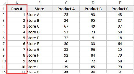
5] Using SUBTOTAL For Filtered Data
Sometimes, you may have a huge dataset, where you want to filter the data and then copy and paste the filtered data into a separate sheet.
If you use any of the methods shown above so far, you will notice that the row numbers remain the same. This means that when you copy the filtered data, you will have to update the row numbering.
In such cases, the SUBTOTAL function can automatically update the row numbers. Even when you filter the data set, the row numbers will remain intact.
Let me show you exactly how it works with an example.
Suppose you have a dataset as shown below:

If I filter this data based on Product A sales, you will get something as shown below:

Note that the serial numbers in Column A are also filtered. So now, you only see the numbers for the rows that are visible.
While this is the expected behavior, in case you want to get a serial row numbering – so that you can simply copy and paste this data somewhere else – you can use the SUBTOTAL function.
Here is the SUBTOTAL function that will make sure that even the filtered data has continuous row numbering.
=SUBTOTAL(3,$B$2:B2)
The 3 in the SUBTOTAL function specifies using the COUNTA function. The second argument is the range on which COUNTA function is applied.
The benefit of the SUBTOTAL function is that it dynamically updates when you filter the data (as shown below):

Note that even when the data is filtered, the row numbering update and remains continuous.
6] Creating an Excel Table
Excel Table is a great tool that you must use when working with tabular data. It makes managing and using data a lot easier.
This is also my favorite method among all the techniques shown in this tutorial.
Let me first show you the right way to number the rows using an Excel Table:
Note that in the formula above, I have used Table2, as that is the name of my Excel table. You can replace Table2 with the name of the table you have.
There are some added benefits of using an Excel Table while numbering rows in Excel:
- Since Excel Table automatically inserts the formula in the entire column, it works when you insert a new row in the Table. This means that when you insert/delete rows in an Excel Table, the row numbering would automatically update (as shown below).

- If you add more rows to the data, Excel Table would automatically expand to include this data as a part of the table. And since the formulas automatically update in the calculated columns, it would insert the row number for the newly inserted row (as shown below).


7] Adding 1 to the Previous Row Number
This is a simple method that works.
The idea is to add 1 to the previous row number (the number in the cell above). This will make sure that subsequent rows get a number that is incremented by 1.
Suppose you have a dataset as shown below:
Here are the steps to enter row numbers using this method:
- In the cell in the first row, enter 1 manually. In this case, it’s in cell A2.
- In cell A3, enter the formula, =A2+1
- Copy and paste the formula for all the cells in the column.

The above steps would enter serial numbers in all the cells in the column. In case there are any blank rows, this would still insert the row number for it.
Also note that in case you insert a new row, the row number would not update. In case you delete a row, all the cells below the deleted row would show a reference error.
These are some quick ways you can use to insert serial numbers in tabular data in Excel.
In case you are using any other method, do share it with me in the comments section.
You May Also Like the Following Excel Tutorials:
- Delete Blank Rows in Excel (with and without VBA).
- How to Insert Multiple Rows in Excel (4 Methods).
- How to Split Multiple Lines in a Cell into a Separate Cells / Columns.
- 7 Amazing Things Excel Text to Columns Can Do For You.
- Highlight EVERY Other ROW in Excel.
- How to Compare Two Columns in Excel.
- Insert New Columns in Excel
How to Add Bullet Points in Excel
You can add numbered lists too
Adding bullet points in Excel can be tricky: Excel doesn’t offer a font-formatting tool for bullets. However, there are many times you may need to add a bullet for each cell, or multiple bullets into each cell. This article looks at the multiple ways you can add bullet points in Excel.
Add Bullet Points in Excel With Shortcut Keys
One of the easiest ways to add bullet points in Excel is using keyboard shortcut keys.
-
To add one bullet point per cell, double-click the first cell where you want a bullet point and press Alt+7 to insert the bullet. Then, type the item you’d like to follow the bullet.
Different keyboard shortcuts will insert different style bullets. For example, Alt+9 creates a hollow bullet; Alt+4 is a diamond; Alt+26 is a right arrow; Alt+254 is a square. The bullet point will only appear after you release the keys.
-
To quickly add bullets before entering a list, select and drag the bottom right corner of the cell down the number of cells you’d like to fill with bullet points before typing text after the bullet.
-
Once you have all of the individual cells filled with bullet points, you can fill them out with the actual item text and the rest of the data for the sheet.
-
If you prefer to include multiple bullets in a single cell, press Alt+Enter after each Alt+7 bullet entry. This will insert a line break into the cell. Continue this process until you’ve entered the number of bullets you need in the cell.
-
Press Enter (without pressing the Alt key) to finish editing the cell. The row height will automatically adjust to accommodate the number of bullet points you’ve entered into the cell.
Add Bullet Points in Excel Using Symbols
If you prefer using your mouse rather than the keyboard to add bullet points in Excel, then Symbols is a great way to go. Using symbols to add bullet points in Excel is ideal if you don’t want to have to remember which shortcuts let you insert specific bullet styles.
-
Select the cell where you want to insert a bullet point, then select Insert > Symbol.
-
Scroll down and select the bullet point symbol. Click Insert.
You don’t necessarily have to use the standard bullet symbol. As you scroll through the list of symbols you may notice many others that make good bullets as well.
-
To insert multiple lines of bullets using symbols, select Insert the number of times you’d like to have bullets, then select Cancel to close the symbol dialogue box. Finally, place the cursor between each bullet in the cell and press Alt+Enter to add a line break between bullets.
Insert a Bullet in Excel Using a Formula
One way to insert bullets in Excel without having to use the menu or remember any keyboard shortcuts is to use Excel’s CHAR function.
The CHAR function will display any character you want, if you provide it with the correct numeric character code. The ASCII character code for a solid bullet point is 149.
There are a limited number of character codes Excel can accept in the CHAR function, and the solid, round bullet point is the only character that makes for a suitable bullet in Excel. If you’re interested in other styles of bullets, then this may not be the right approach for you.
-
Double-click the cell where you want to insert a bullet list, then type «=CHAR(149).»
-
Press Enter and the formula will turn into a bullet point.
-
To insert multiple lines of bullet points in Excel using formulas, include another CHAR function using the line break code, which is 10. Double-click the cell to edit and type «=CHAR(149)&CHAR(10)&CHAR(149).»
-
When you press Enter, you’ll see the bullet points on each line. You may need to adjust the height of the row to see them all.
Add Bullets to Excel With Shapes
Inserting shapes as bullet points is a creative way to use images of different shapes or colors as bullet points.
-
Select Insert > Shapes. You’ll see a drop-down list of all of the available shapes you have to choose from.
-
Select the shape you’d like to use as your bullet, and it will appear on the spreadsheet. Select the shape, then resize it appropriately to fit inside each row.
-
Drag the icon into the first row. Then, select, copy, and paste copies of it into the rows below it.
-
Combine each cell that contains a bullet icon with the second cell that contains the text.
Using Bullets in Text Boxes
Excel provides bullet-formatting functionality buried within specific tools such as Text Box. Text box bullet lists work as they do in a Word document.
-
To use bullet lists inside a text box, select Insert > Text Box, then draw the text box anywhere into the spreadsheet.
-
Right-click anywhere in the text box, select the arrow next to the Bullets item, then select the bullet style you want to use.
-
Once the bullet list is created in the text box, you can type in each item and press Enter to move to the next bullet item.
Adding SmartArt Bullet Lists in Excel
Hidden deep inside Excel’s SmartArt Graphic list are several graphical bullet lists that you can insert into any spreadsheet.
-
Select Insert > SmartArt to open the Choose a SmartArt Graphic dialog box.
-
Select List from the left menu. Here, you’ll find an array of formatted list graphics you can use to add bullets in your spreadsheet.
-
Select any one of these and select OK to finish. This will insert the graphic into your spreadsheet in design mode. Enter the text for your list into each header and line item.
-
When you’re finished, select anywhere in the sheet to finish. You can also select and move the graphic to place it wherever you like.
Adding Numbered Lists in Excel
Adding a numbered list in Excel is very easy using the fill feature.
-
When creating your list, first type 1 in the first row where you want to start the numbered list. Then, type 2 in the row just below it.
-
Highlight both numbered cells, then place your mouse pointer over the small box in the lower right of the second cell. The mouse icon will change to a small crosshair. Select and drag the mouse down the number of rows of items you’d like to have in your list.
-
When you release the mouse button, all cells will automatically fill with the numbered list.
-
Now you can complete your list by filling in the cells to the right of your numbered list.
How to Make Numbered Symbol Lists in Excel
You can also use symbols to create numbered lists in Excel. This method creates much more stylistic numbered lists, but it can be a bit more tedious than the autofill option.
-
Using the example above, delete all of the numbers in the left column.
-
Select inside the first cell, then select Insert > Symbols > Symbol.
-
Select one of the numbered symbols for the number one, and select Insert to insert that symbol into the first cell.
-
Select Close, select the next cell, then repeat the process above, selecting each subsequent number symbol—two for the second cell, three for the third cell, and so on.
Thanks for letting us know!
Get the Latest Tech News Delivered Every Day
Subscribe