
Open Shapes on the Insert tab and select the double arrow line. You’ll use this to draw the base line. Position the cursor cross where you want the line to start, hold down the Shift key to keep the line straight and drag across the spreadsheet horizontally to the point where it should stop.
Contents
- 1 How do I auto number a column in Excel?
- 2 What is a number line example?
- 3 How do you autofill in numbers?
- 4 How do I insert a specific row in Excel?
- 5 How do you represent 2.5 on a number line?
- 6 Where does 1.4 go on a number line?
- 7 How does a number line look like?
- 8 How do you use the row number in Excel?
- 9 What is row number in Excel?
- 10 How do you show row numbers in Excel?
- 11 How do I AutoFill numbers in Excel without dragging?
- 12 Where is AutoFill options in Excel?
- 13 Where is AutoFill in Excel?
- 14 How do I make multiple lines in one cell in Excel?
- 15 How do I insert a large number of rows in Excel?
- 16 How do you represent 2.4 on a number line?
- 17 How do you represent 7 upon 4 on a number line?
- 18 What is 4/5 as a number?
- 19 How do you represent 1.3 on a number line?
- 20 How do you represent 2.3 on a number line?
How do I auto number a column in Excel?
Auto number a column by AutoFill function
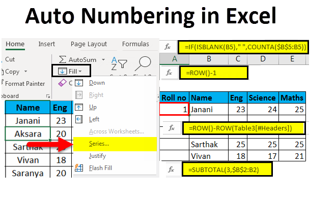
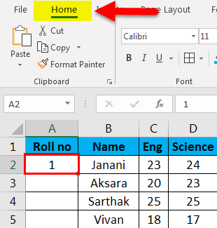
Type 1 into a cell that you want to start the numbering, then drag the autofill handle at the right-down corner of the cell to the cells you want to number, and click the fill options to expand the option, and check Fill Series, then the cells are numbered.
What is a number line example?
An example of a number line is what a math student can use to find the answer to addition and subtraction questions.A straight line, theoretically extending to infinity in both positive and negative directions from zero, that shows the relative order of the real numbers.
How do you autofill in numbers?
Do one of the following: Autofill one or more cells with content from adjacent cells: Select the cells with the content you want to copy, then move the pointer over a border of the selection until a yellow autofill handle (a dot) appears. Drag the handle over the cells where you want to add the content.
How do I insert a specific row in Excel?
Insert rows
- Select the heading of the row above where you want to insert additional rows. Tip: Select the same number of rows as you want to insert.
- Hold down CONTROL, click the selected rows, and then on the pop-up menu, click Insert. Tip: To insert rows that contain data, see Copy and paste specific cell contents.
How do you represent 2.5 on a number line?
(d) We know that, 2.5 is more than 2 but less than 3. There are 2 ones and 5 tenths in it. Divide the unit length between 0 and 1, 1 and 2, 2 and 3 into 10 equal parts and take 5 parts, which represents 2.5 = (2 + 0.5) as shown below on the number line.
Where does 1.4 go on a number line?
0.5 can be written as 5/10. So, five tenths is the 5 th part from zero. Similarly 1.4 can be written as 14/10. So fourteen tenths is fourteenth part from zero. or fourth part from one.
How does a number line look like?
A number line is just that – a straight, horizontal line with numbers placed at even increments along the length. It’s not a ruler, so the space between each number doesn’t matter, but the numbers included on the line determine how it’s meant to be used. A number ladder is the vertical version of a number line.
How do you use the row number in Excel?
Use the ROW function to number rows
- In the first cell of the range that you want to number, type =ROW(A1). The ROW function returns the number of the row that you reference. For example, =ROW(A1) returns the number 1.
- Drag the fill handle. across the range that you want to fill.
What is row number in Excel?
Reference is the argument accepted by the ROW formula excel which is a cell or range of cells for which we want the row number.
Row Formula Excel.
| Argument Value | Cell Formula | Explanation |
|---|---|---|
| A Cell Reference | 1 | Returnsthe ROW number 1 |
| A Range | 2 | Returns the Row number 2 |
How do you show row numbers in Excel?
If you need a quick way to count rows that contain data, select all the cells in the first column of that data (it may not be column A). Just click the column header. The status bar, in the lower-right corner of your Excel window, will tell you the row count.
How do I AutoFill numbers in Excel without dragging?
The regular way of doing this is: Enter 1 in cell A1. Enter 2 in cell A2. Select both the cells and drag it down using the fill handle.
Quickly Fill Numbers in Cells without Dragging
- Enter 1 in cell A1.
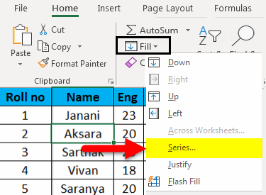
- Go to Home –> Editing –> Fill –> Series.
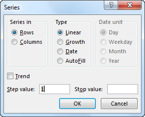
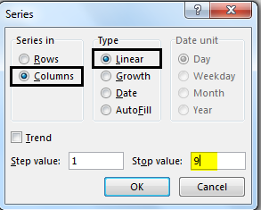
- In the Series dialogue box, make the following selections:
- Click OK.
Where is AutoFill options in Excel?
The Fill button is located in the Editing group right below the AutoSum button (the one with the Greek sigma). When you select the Series option, Excel opens the Series dialog box. Click the AutoFill option button in the Type column followed by the OK button in the Series dialog box.
Where is AutoFill in Excel?
Select cell A1 and cell A2 and drag the fill handle down. The fill handle is the little green box at the lower right of a selected cell or selected range of cells. Note: AutoFill automatically fills in the numbers based on the pattern of the first two numbers.
How do I make multiple lines in one cell in Excel?
You can put multiple lines in a cell with pressing Alt + Enter keys simultaneously while entering texts. Pressing the Alt + Enter keys simultaneously helps you separate texts with different lines in one cell. With this shortcut key, you can split the cell contents into multiple lines at any position as you need.
How do I insert a large number of rows in Excel?
To insert multiple rows, select the same number of rows that you want to insert. To select multiple rows hold down the “shift” key on your keyboard on a Mac or PC. For example, if you want to insert six rows, select six rows while holding the “shift” key.
How do you represent 2.4 on a number line?
1st draw a line from -4 to any no. and then circle 2.4 between -3 and -2.
How do you represent 7 upon 4 on a number line?
How to represent 7/4 on the number line?
- Divide the line between the whole numbers into 4 parts. i.e., divide the line between 0 and 1 to 4 parts, 1 and 2 to 4 parts and so on.
- Thus, the rational number 7/4 lies at a distance of 7 points away from 0 towards the positive number line.
What is 4/5 as a number?
0.8
Answer: 4/5 as a decimal is 0.8.
How do you represent 1.3 on a number line?
First step is to draw a number line and divide the space between every pair of the consecutive integers like 0 and 1, 1 and 2 on the number line in 10 equal parts. In order to represent 1.3 i.e move three parts on the right-side of one or we can say move thirteen parts on the right side of zero.
How do you represent 2.3 on a number line?
Step-by-step explanation:
- Mark a line segment OA = 2.3 cm on number line.
- Mark B at a distance of 1 unit from A.
- Find the midpoint of OB and mark it point C.
- Draw a semi-circle OB while taking C as its center.
- Draw a perpendicular to line OB passing through point A.
- Let it intersect the semi-circle at D.
See all How-To Articles
This tutorial demonstrates how to make a number line in Excel and Google Sheets.
Make a Number Line
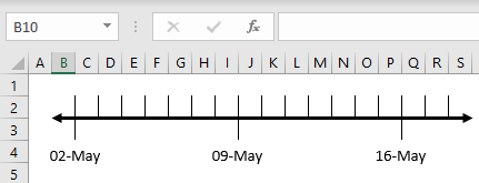
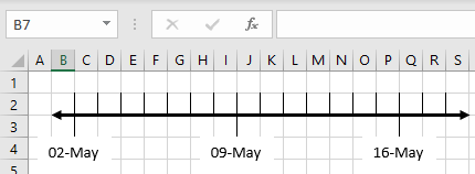
Using Excel, you can create a number line that can be used to display a timeline. Say you want to create a timeline, displaying a couple of weeks, with days included.
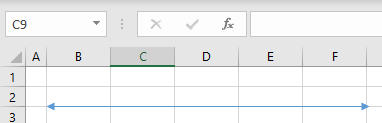
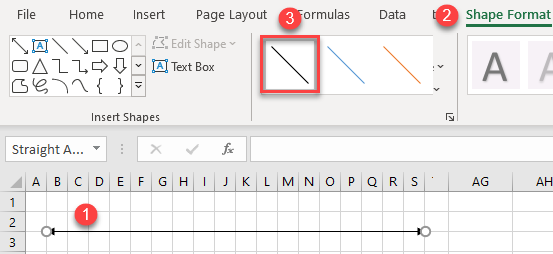
- To insert a line, in the Ribbon, go to Insert > Shapes, and choose a line with arrows on both ends.
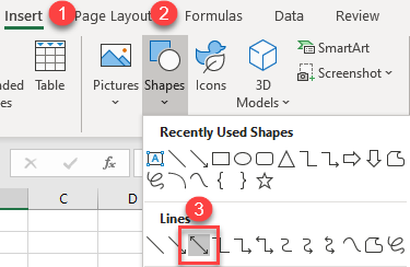
- Click where you want to start the line, hold down the SHIFT key (to keep it straight), and draw the line.
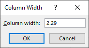
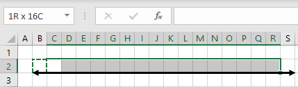
- To have equal spaces between days, resize the column widths. Select the columns you need, right-click anywhere in the selection, and choose Column Width…
(Every cell is one day, so for this example, select 18 columns.)
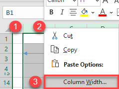
- Type in a smaller column width (2.29) and click OK.
- Now you have cells formatted as small squares.
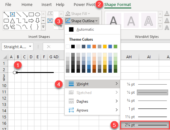
Select the line, and in the Ribbon, go to the Shape Format tab, and choose black for the color.
- In the Ribbon, go to the Shape Format > Shape Outline > Weight and choose a thicker line style (here, 2 ¼ pt).
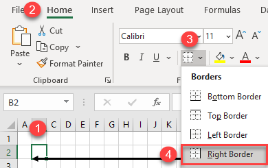
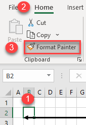
- Now, draw small vertical lines, to represent days, above the main horizontal line. This can be done using the cells’ borders. Select the first cell above the line (B2) and in the Ribbon, go to the Home tab. Click the arrow next to the Borders icon and choose Right Border.
- Use the format painter to apply the border to the other cells. Select the first cell (B2) and in the Ribbon, go to Home > Format Painter.
- Select the rest of the cells above the line to insert a right border for each cell.
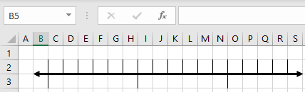
- Repeat Steps 8 and 9 to create a right border for each seventh cell under the line. These lines represent the first day of each week.
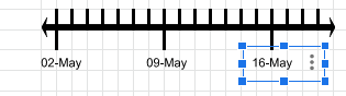
- Insert text boxes for dates at the beginning of each week. In the Ribbon, go to Insert > Text Box.
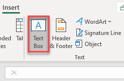
- Draw and resize the text box under the first line. Type in the first date (02-May).
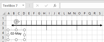
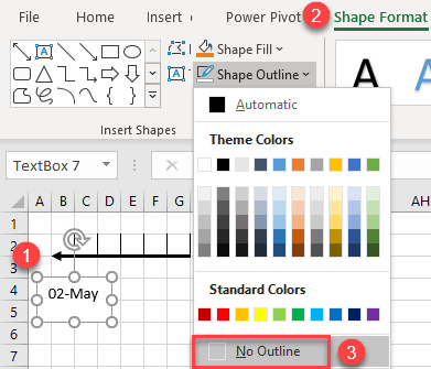
- To remove the text box outline, select the text box and in the Ribbon, go to Shape Format > Shape Outline > No Outline.
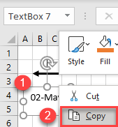
- Now copy the text box. Right-click the text box’s border and choose Copy (or use the keyboard shortcut CTRL + C).
- Position the cursor under the second week line, right-click, and choose Paste (or use the keyboard shortcut CTRL + V).
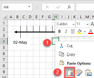
- Type in the next week’s date (09-May) and repeat Steps 14 and 15 to insert the third text box (16-May).
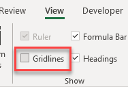
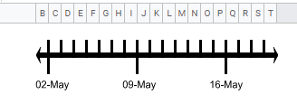
- Hide the gridlines to show only the number line. In the Ribbon, go to the View tab, and uncheck Gridlines.
As a result, you have the number line with days and weeks marked.
Number Line in Google Sheets
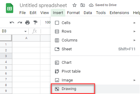
To create a number line in Google Sheets, first create a line in a drawing, and then insert that into your sheet.
- In the Menu, go to Insert > Drawing.
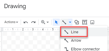
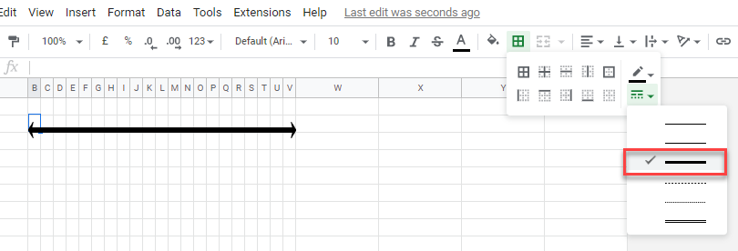
- In the Toolbar, click Line, and then drag to draw a straight line.
- Add a left arrow head to the line, then a right arrow head.
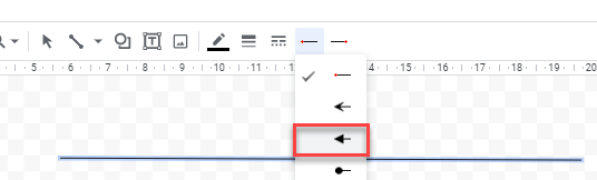
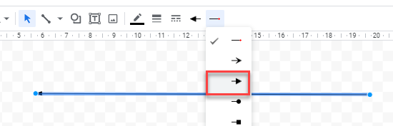
- Click Save and close to return to your Google sheet.

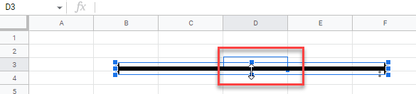
- Resize the line by selecting it and dragging down with your mouse.
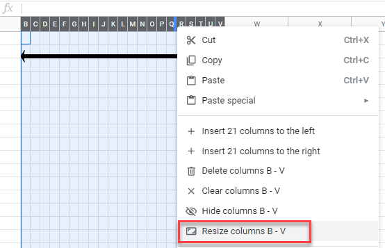
- Now, resize the columns in your Google sheet.
Select the columns to resize and right-click on the column header. Select Resize columns in the quick menu.
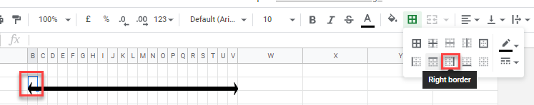
- Now insert right-hand borders for each cell in your number line.
From the Toolbar, set the width of the border.
- Then, choose Right border for each cell on the number line.
-
- Once you have set all the right-hand cell borders (days), draw a text box. Once again, this involves inserting a drawing. In the Drawing window, click Text box.
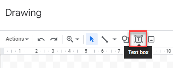
- Then type in the date and click Save and close.
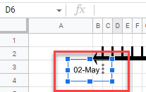
- Repeat Steps 10 and 11 to create the other text boxes.
- Finally, in the View menu, switch gridlines off.
Primary Navigation Menu

Contents
- Method 1: Numbering After Filling in the First Lines
- Method 2: “ROW” operator
- Method 3: applying progression
- Conclusion
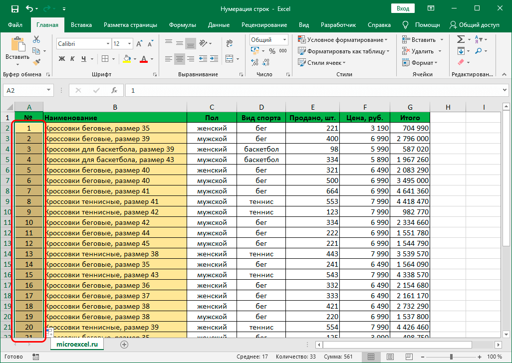
When working with a table, numbering may be necessary. It structures, allows you to quickly navigate in it and search for the necessary data. Initially, the program already has numbering, but it is static and cannot be changed. A way to manually enter numbering is provided, which is convenient, but not as reliable, it is difficult to use when working with large tables. Therefore, in this article, we will look at three useful and easy-to-use ways to number tables in Excel.
Method 1: Numbering After Filling in the First Lines
This method is the simplest and most commonly used when working with small and medium tables. It takes a minimum of time and guarantees the elimination of any errors in the numbering. Their step by step instructions are as follows:
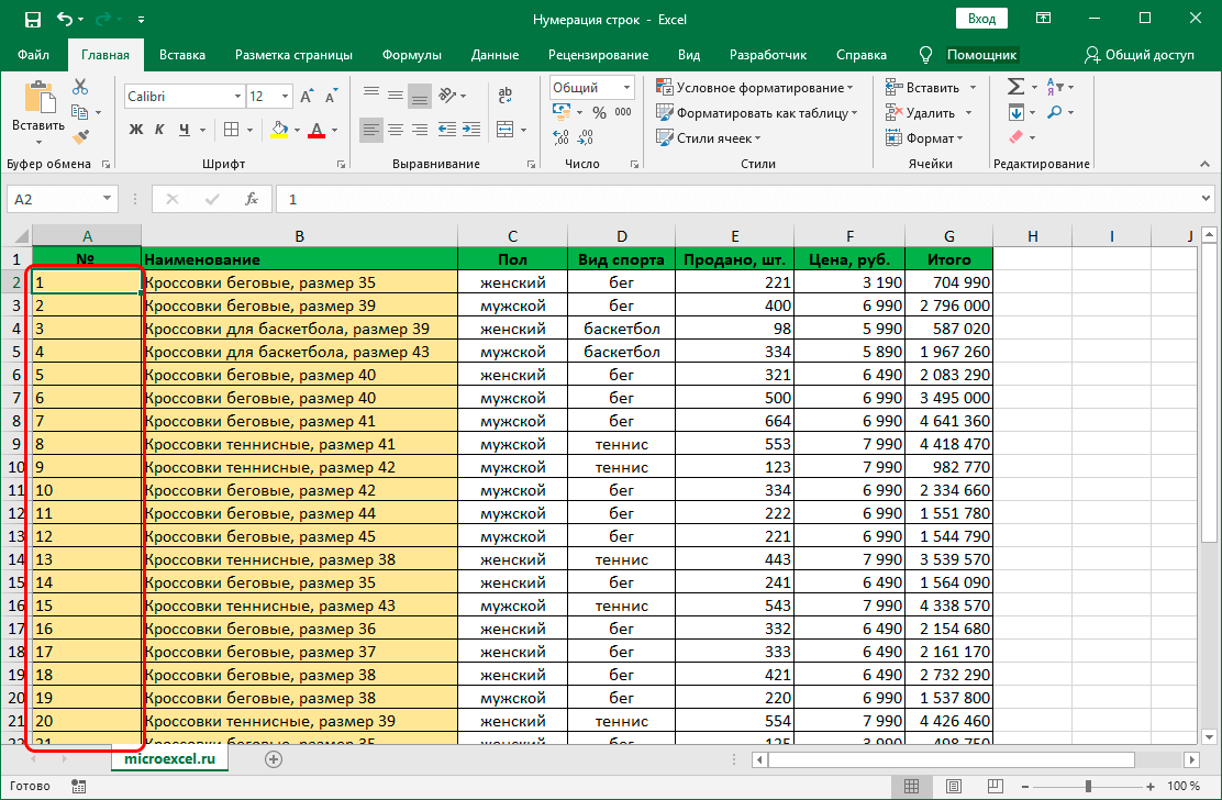
- First you need to create an additional column in the table, which will be used for further numbering.
- Once the column is created, put the number 1 on the first row, and put the number 2 on the second row.
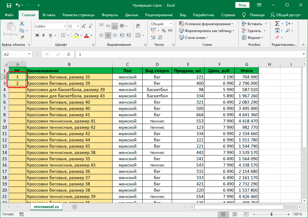
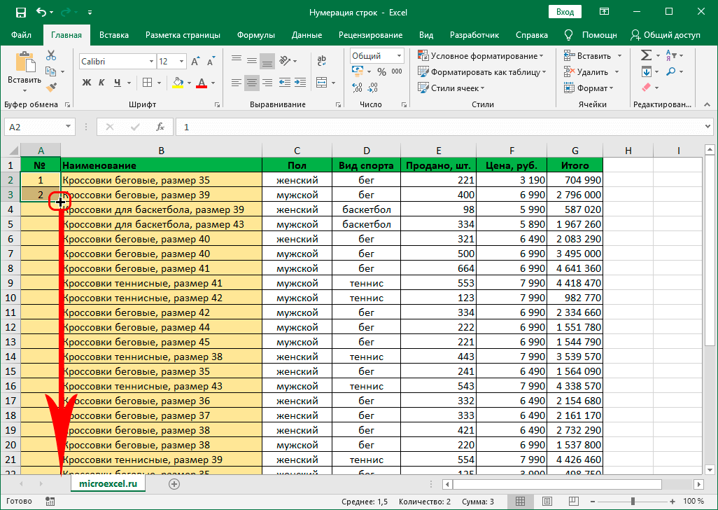
- Select the filled two cells and hover over the lower right corner of the selected area.
- As soon as the black cross icon appears, hold LMB and drag the area to the end of the table.
If everything is done correctly, then the numbered column will be automatically filled. This will be enough to achieve the desired result.
Method 2: “ROW” operator
Now let’s move on to the next numbering method, which involves the use of the special “STRING” function:
- First, create a column for numbering, if one does not exist.
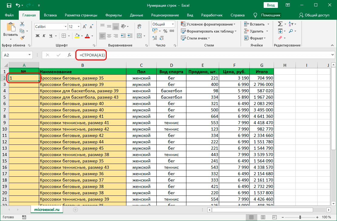
- In the first row of this column, enter the following formula: =ROW(A1).
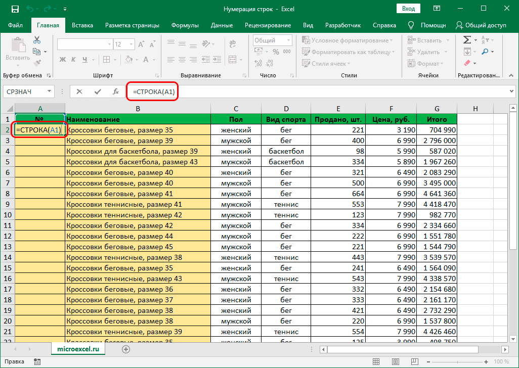
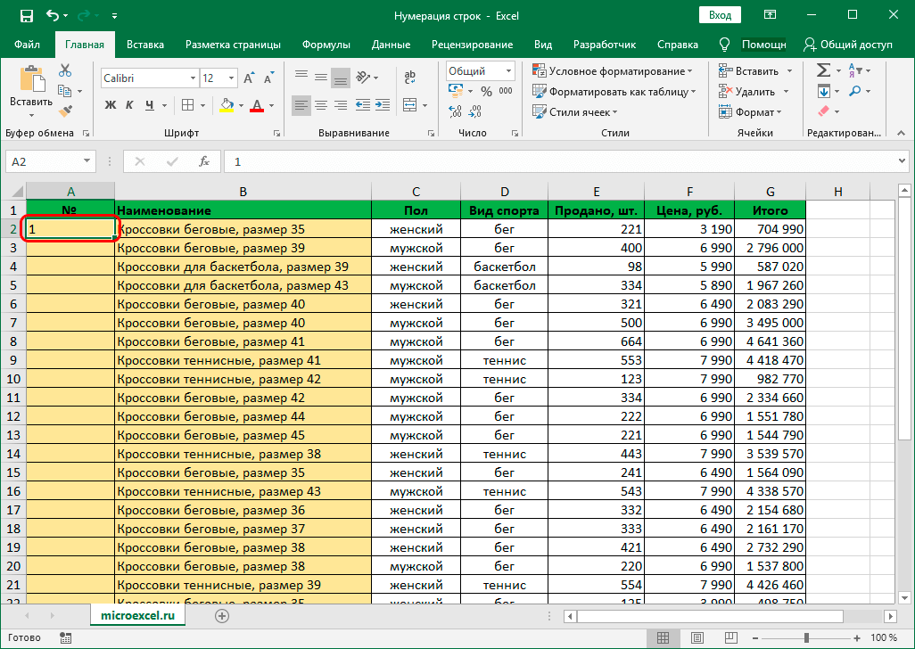
- After entering the formula, be sure to press the “Enter” key, which activates the function, and you will see the number 1.
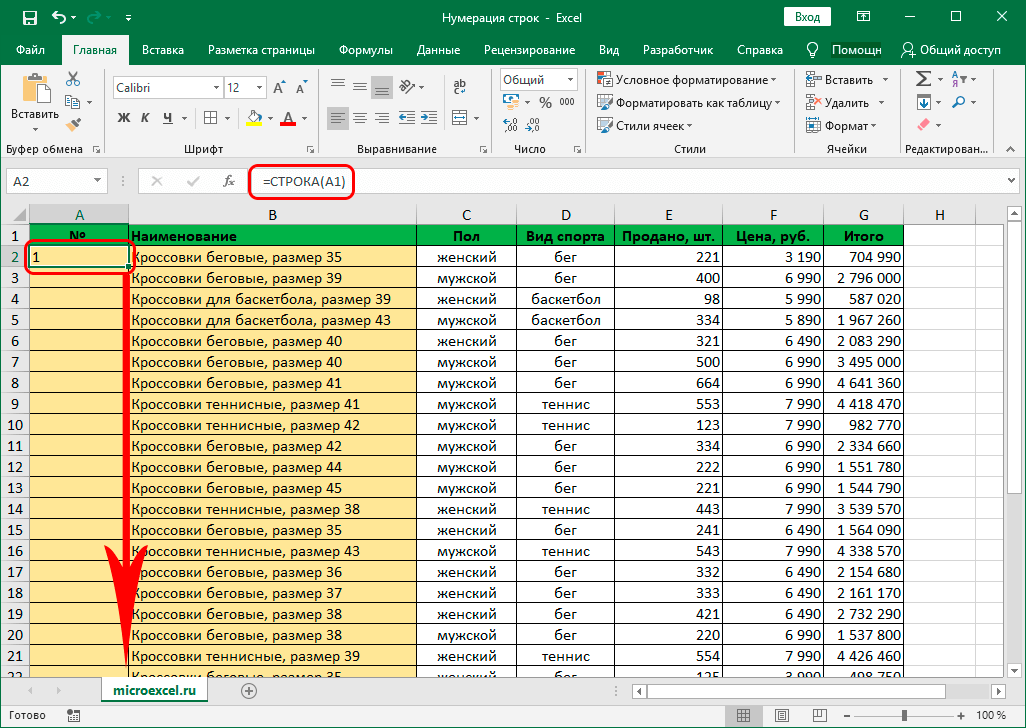
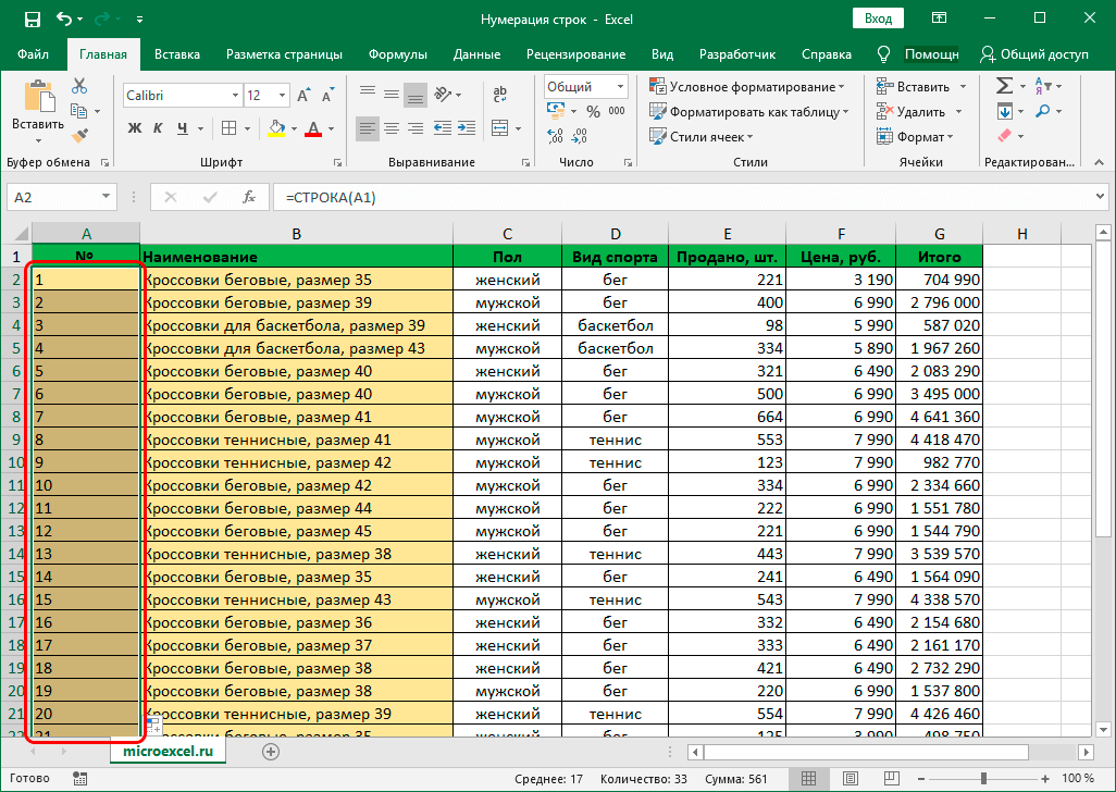
- Now it remains, similarly to the first method, to move the cursor to the lower right corner of the selected area, wait for the black cross to appear and stretch the area to the end of your table.
- If everything is done correctly, then the column will be filled with numbering and can be used for further information retrieval.
There is an alternative method, in addition to the specified method. True, it will require the use of the “Function Wizard” module:
- Similarly create a column for numbering.
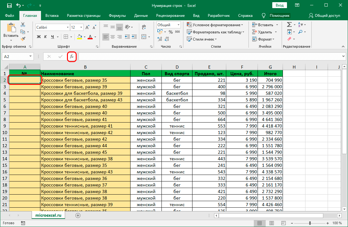
- Click on the first cell in the first row.
- At the top near the search bar, click on the “fx” icon.
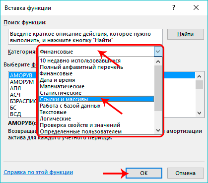
- The “Function Wizard” is activated, in which you need to click on the “Category” item and select “References and Arrays”.
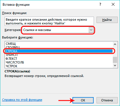
- From the proposed functions, it remains to select the option “ROW”.
- An additional window for entering information will appear. You need to put the cursor in the “Link” item and in the field indicate the address of the first cell of the numbering column (in our case, this is the value A1).
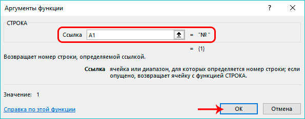
- Thanks to the actions performed, the number 1 will appear in the empty first cell. It remains to use the lower right corner of the selected area again to drag it to the entire table.
These actions will help you get all the necessary numbering and help you not to be distracted by such trifles while working with the table.
Method 3: applying progression
This method differs from others in that eliminates the need for users to use an autofill token. This question is extremely relevant, since its use is inefficient when working with huge tables.
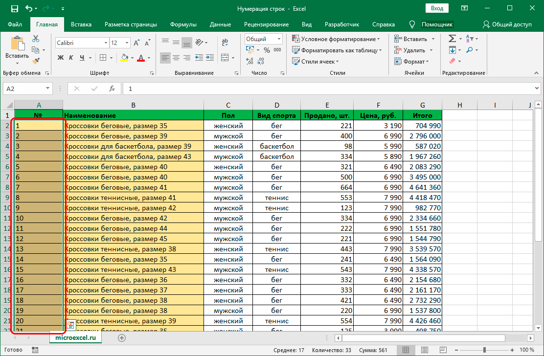
- We create a column for numbering and mark the number 1 in the first cell.
- We go to the toolbar and use the “Home” section, where we go to the “Editing” subsection and look for the icon in the form of a down arrow (when hovering over, it will give the name “Fill”).
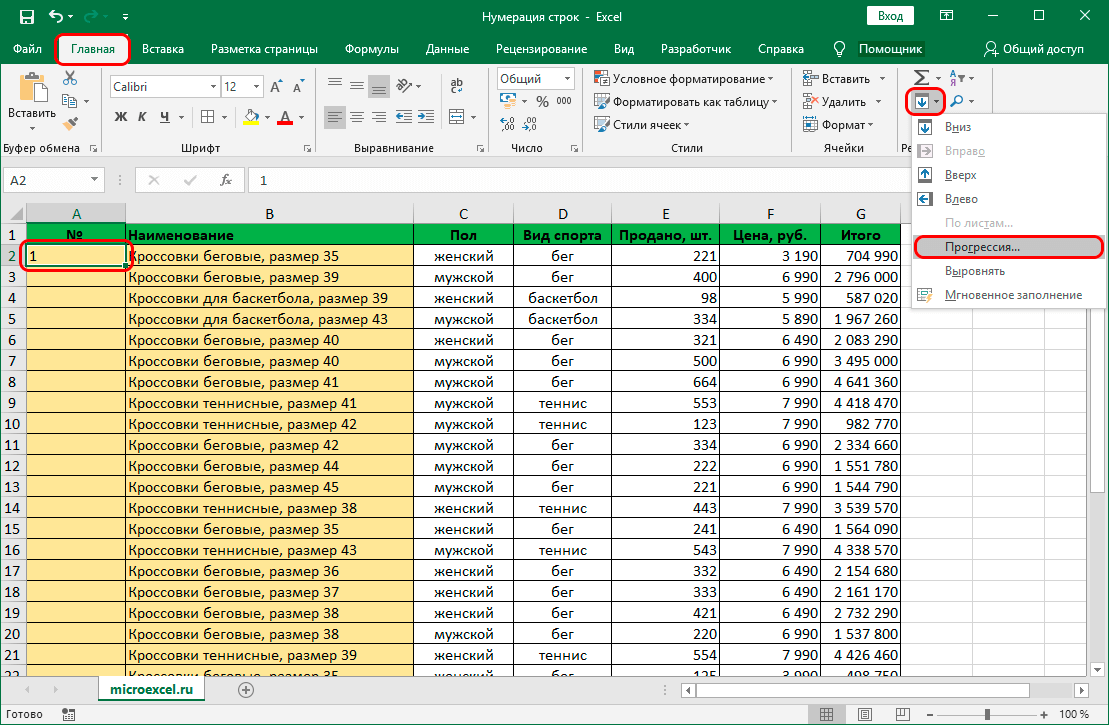
- In the drop-down menu, you need to use the “Progression” function.
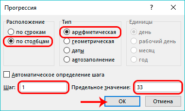
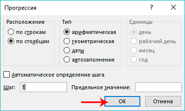
- In the window that appears, do the following:
- mark the value “By columns”;
- select arithmetic type;
- in the “Step” field, mark the number 1;
- in the paragraph “Limit value” you should note how many lines you plan to number.
- If everything is done correctly, then you will see the result of automatic numbering.
There is an alternative way to do this numbering, which looks like this:
- Repeat the steps to create a column and mark in the first cell.
- Select the entire range of the table that you plan to number.
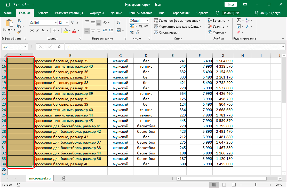
- Go to the “Home” section and select the “Editing” subsection.
- We are looking for the item “Fill” and select “Progression”.
- In the window that appears, we note similar data, although now we do not fill in the “Limit value” item.
- Click on “OK”.
This option is more universal, since it does not require mandatory counting of lines that need numbering. True, in any case, you will have to select the range that needs to be numbered.
Pay attention! In order to make it easier to select a range of a table followed by numbering, you can simply select a column by clicking on the Excel header. Then use the third numbering method and copy the table to a new sheet. This will simplify the numbering of huge tables.
Conclusion
Line numbering can make it easier to work with a table that needs constant updating or needs to find the information you need. Thanks to the detailed instructions above, you will be able to choose the most optimal solution for the task at hand.
2022-08-15
Automatically number rows
Unlike other Microsoft 365 programs, Excel does not provide a button to number data automatically. But, you can easily add sequential numbers to rows of data by dragging the fill handle to fill a column with a series of numbers or by using the ROW function.
Tip: If you are looking for a more advanced auto-numbering system for your data, and Access is installed on your computer, you can import the Excel data to an Access database. In an Access database, you can create a field that automatically generates a unique number when you enter a new record in a table.

What do you want to do?
-
Fill a column with a series of numbers
-
Use the ROW function to number rows
-
Display or hide the fill handle
Fill a column with a series of numbers
-
Select the first cell in the range that you want to fill.
-
Type the starting value for the series.
-
Type a value in the next cell to establish a pattern.
Tip: For example, if you want the series 1, 2, 3, 4, 5…, type 1 and 2 in the first two cells. If you want the series 2, 4, 6, 8…, type 2 and 4.
-
Select the cells that contain the starting values.
Note: In Excel 2013 and later, the Quick Analysis button is displayed by default when you select more than one cell containing data. You can ignore the button to complete this procedure.
-
Drag the fill handle
 across the range that you want to fill.
Note: As you drag the fill handle across each cell, Excel displays a preview of the value. If you want a different pattern, drag the fill handle by holding down the right-click button, and then choose a pattern.
To fill in increasing order, drag down or to the right. To fill in decreasing order, drag up or to the left.
Tip: If you do not see the fill handle, you may have to display it first. For more information, see Display or hide the fill handle.
Note: These numbers are not automatically updated when you add, move, or remove rows. You can manually update the sequential numbering by selecting two numbers that are in the right sequence, and then dragging the fill handle to the end of the numbered range.
Use the ROW function to number rows
-
In the first cell of the range that you want to number, type =ROW(A1).
The ROW function returns the number of the row that you reference. For example, =ROW(A1) returns the number 1.
-
Drag the fill handle
across the range that you want to fill.Tip: If you do not see the fill handle, you may have to display it first. For more information, see Display or hide the fill handle.
-
These numbers are updated when you sort them with your data. The sequence may be interrupted if you add, move, or delete rows. You can manually update the numbering by selecting two numbers that are in the right sequence, and then dragging the fill handle to the end of the numbered range.
-
If you are using the ROW function, and you want the numbers to be inserted automatically as you add new rows of data, turn that range of data into an Excel table. All rows that are added at the end of the table are numbered in sequence. For more information, see Create or delete an Excel table in a worksheet.
To enter specific sequential number codes, such as purchase order numbers, you can use the ROW function together with the TEXT function. For example, to start a numbered list by using 000-001, you enter the formula =TEXT(ROW(A1),»000-000″) in the first cell of the range that you want to number, and then drag the fill handle to the end of the range.
Display or hide the fill handle
The fill handle  displays by default, but you can turn it on or off.
-
In Excel 2010 and later, click the File tab, and then click Options.
In Excel 2007, click the Microsoft Office Button
, and then click Excel Options. -
In the Advanced category, under Editing options, select or clear the Enable fill handle and cell drag-and-drop check box to display or hide the fill handle.
 , and then click Excel Options.
Note: To help prevent replacing existing data when you drag the fill handle, ensure the Alert before overwriting cells check box is selected. If you do not want Excel to display a message about overwriting cells, you can clear this check box.
See Also
Overview of formulas in Excel
How to avoid broken formulas
Find and correct errors in formulas
Excel keyboard shortcuts and function keys
Lookup and reference functions (reference)
Excel functions (alphabetical)
Excel functions (by category)
Need more help?
Watch Video – 7 Quick and Easy Ways to Number Rows in Excel
When working with Excel, there are some small tasks that need to be done quite often. Knowing the ‘right way’ can save you a great deal of time.
One such simple (yet often needed) task is to number the rows of a dataset in Excel (also called the serial numbers in a dataset).
Now if you’re thinking that one of the ways is to simply enter these serial number manually, well – you’re right!
But that’s not the best way to do it.
Imagine having hundreds or thousands of rows for which you need to enter the row number. It would be tedious – and completely unnecessary.
There are many ways to number rows in Excel, and in this tutorial, I am going to share some of the ways that I recommend and often use.
Of course, there would be more, and I will be waiting – with a coffee – in the comments area to hear from you about it.
How to Number Rows in Excel
The best way to number the rows in Excel would depend on the kind of data set that you have.
For example, you may have a continuous data set that starts from row 1, or a dataset that start from a different row. Or, you might have a dataset that has a few blank rows in it, and you only want to number the rows that are filled.
You can choose any one of the methods that work based on your dataset.
1] Using Fill Handle
Fill handle identifies a pattern from a few filled cells and can easily be used to quickly fill the entire column.
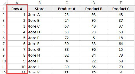
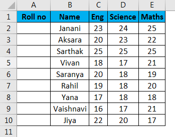
Suppose you have a dataset as shown below:

Here are the steps to quickly number the rows using the fill handle:
Note that Fill Handle automatically identifies the pattern and fill the remaining cells with that pattern. In this case, the pattern was that the numbers were getting incrementing by 1.
In case you have a blank row in the dataset, fill handle would only work till the last contiguous non-blank row.
Also, note that in case you don’t have data in the adjacent column, double-clicking the fill handle would not work. You can, however, place the cursor on the fill handle, hold the right mouse key and drag down. It will fill the cells covered by the cursor dragging.
2] Using Fill Series
While Fill Handle is a quick way to number rows in Excel, Fill Series gives you a lot more control over how the numbers are entered.
Suppose you have a dataset as shown below:
Here are the steps to use Fill Series to number rows in Excel:
This will instantly number the rows from 1 to 26.
Using ‘Fill Series’ can be useful when you’re starting by entering the row numbers. Unlike Fill Handle, it doesn’t require the adjacent columns to be filled already.
Even if you have nothing on the worksheet, Fill Series would still work.
Note: In case you have blank rows in the middle of the dataset, Fill Series would still fill the number for that row.
3] Using the ROW Function
You can also use Excel functions to number the rows in Excel.
In the Fill Handle and Fill Series methods above, the serial number inserted is a static value. This means that if you move the row (or cut and paste it somewhere else in the dataset), the row numbering will not change accordingly.
This shortcoming can be tackled using formulas in Excel.
You can use the ROW function to get the row numbering in Excel.
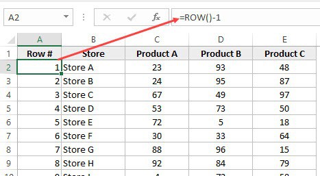
To get the row numbering using the ROW function, enter the following formula in the first cell and copy for all the other cells:
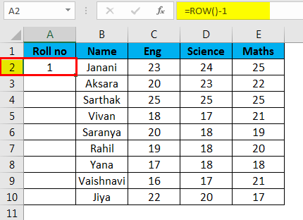
=ROW()-1
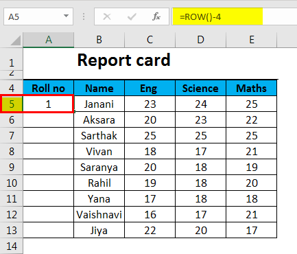
The ROW() function gives the row number of the current row. So I have subtracted 1 from it as I started from the second row onwards. If your data starts from the 5th row, you need to use the formula =ROW()-4.
The best part about using the ROW function is that it will not screw up the numberings if you delete a row in your dataset.
Since the ROW function is not referencing any cell, it will automatically (or should I say AutoMagically) adjust to give you the correct row number. Something as shown below:

Note that as soon as I delete a row, the row numbers automatically update.
Again, this would not take into account any blank records in the dataset. In case you have blank rows, it will still show the row number.
You can use the following formula to hide the row number for blank rows, but it would still not adjust the row numbers (such that the next row number is assigned to the next filled row).
IF(ISBLANK(B2),"",ROW()-1)
4] Using the COUNTA Function
If you want to number rows in a way that only the ones that are filled get a serial number, then this method is the way to go.
It uses the COUNTA function that counts the number of cells in a range that are not empty.
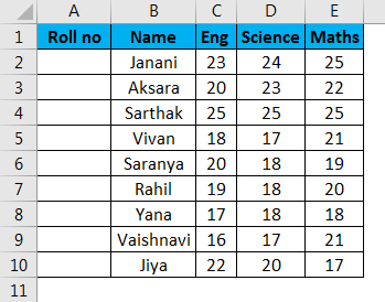
Suppose you have a dataset as shown below:
Note that there are blank rows in the above-shown dataset.
Here is the formula that will number the rows without numbering the blank rows.
=IF(ISBLANK(B2),"",COUNTA($B$2:B2))
The IF function checks whether the adjacent cell in column B is empty or not. If it’s empty, it returns a blank, but if it’s not, it returns the count of all the filled cells till that cell.
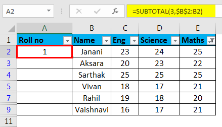
5] Using SUBTOTAL For Filtered Data
Sometimes, you may have a huge dataset, where you want to filter the data and then copy and paste the filtered data into a separate sheet.
If you use any of the methods shown above so far, you will notice that the row numbers remain the same. This means that when you copy the filtered data, you will have to update the row numbering.
In such cases, the SUBTOTAL function can automatically update the row numbers. Even when you filter the data set, the row numbers will remain intact.
Let me show you exactly how it works with an example.
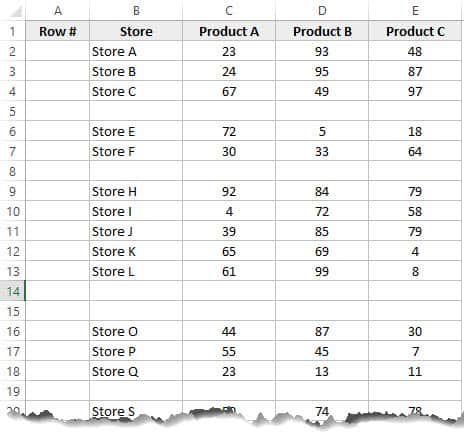
Suppose you have a dataset as shown below:

If I filter this data based on Product A sales, you will get something as shown below:

Note that the serial numbers in Column A are also filtered. So now, you only see the numbers for the rows that are visible.
While this is the expected behavior, in case you want to get a serial row numbering – so that you can simply copy and paste this data somewhere else – you can use the SUBTOTAL function.
Here is the SUBTOTAL function that will make sure that even the filtered data has continuous row numbering.
=SUBTOTAL(3,$B$2:B2)
The 3 in the SUBTOTAL function specifies using the COUNTA function. The second argument is the range on which COUNTA function is applied.
The benefit of the SUBTOTAL function is that it dynamically updates when you filter the data (as shown below):

Note that even when the data is filtered, the row numbering update and remains continuous.
6] Creating an Excel Table
Excel Table is a great tool that you must use when working with tabular data. It makes managing and using data a lot easier.
This is also my favorite method among all the techniques shown in this tutorial.
Let me first show you the right way to number the rows using an Excel Table:
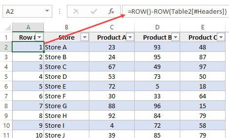
Note that in the formula above, I have used Table2, as that is the name of my Excel table. You can replace Table2 with the name of the table you have.
There are some added benefits of using an Excel Table while numbering rows in Excel:
- Since Excel Table automatically inserts the formula in the entire column, it works when you insert a new row in the Table. This means that when you insert/delete rows in an Excel Table, the row numbering would automatically update (as shown below).

- If you add more rows to the data, Excel Table would automatically expand to include this data as a part of the table. And since the formulas automatically update in the calculated columns, it would insert the row number for the newly inserted row (as shown below).


7] Adding 1 to the Previous Row Number
This is a simple method that works.
The idea is to add 1 to the previous row number (the number in the cell above). This will make sure that subsequent rows get a number that is incremented by 1.
Suppose you have a dataset as shown below:
Here are the steps to enter row numbers using this method:
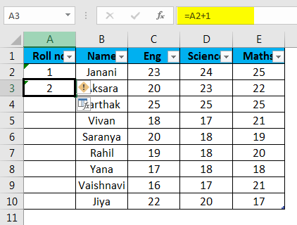
- In the cell in the first row, enter 1 manually. In this case, it’s in cell A2.
- In cell A3, enter the formula, =A2+1
- Copy and paste the formula for all the cells in the column.

The above steps would enter serial numbers in all the cells in the column. In case there are any blank rows, this would still insert the row number for it.
Also note that in case you insert a new row, the row number would not update. In case you delete a row, all the cells below the deleted row would show a reference error.
These are some quick ways you can use to insert serial numbers in tabular data in Excel.
In case you are using any other method, do share it with me in the comments section.
You May Also Like the Following Excel Tutorials:
- Delete Blank Rows in Excel (with and without VBA).
- How to Insert Multiple Rows in Excel (4 Methods).
- How to Split Multiple Lines in a Cell into a Separate Cells / Columns.
- 7 Amazing Things Excel Text to Columns Can Do For You.
- Highlight EVERY Other ROW in Excel.
- How to Compare Two Columns in Excel.
- Insert New Columns in Excel
Using Excel as a Graphic Organizer:
Making a Number Line
Using Excel as a graphic organizer, you can create a variety of documents useful in a classroom. This module will discuss how to create a number line. The number line can be printed and used as a worksheet. However, if viewed in Excel you have some interactive possibilities. If you have classroom projection capability, or an interactive whiteboard, this number line can be really useful.
Open an Excel workbook. Click on the column heading
A
. The entire column will highlight. Scroll over to the right until you can see column heading
Z
. Hold down your shift key and click on the Z. You should now have 26 columns selected. Click on the line between any two column heading letters and drag to the left until the column width is approximately
3
(26 pixels). When you release the mouse button all 26 columns will be the same narrow width. Scroll back to column A and click anywhere to remove the highlight color. We will use these grid lines as reference points for our number line.
To make the number line you will draw one long thick horizontal line with arrows on both ends. All other lines will be created with the
Borders
toolbar button. You must have the
Drawing
toolbar open to draw this line. If the toolbar is not open, go to the
View
menu, select
Toolbars
and slide over to
Drawing
and click one time.
Click on the word
AutoShapes
in the
Drawing
toolbar, move your cursor to
Lines
and click one time on the line with two arrow heads.
Move your cross hair cursor somewhere near the middle of the sheet, close to the left edge. Place your cross hair cursor on the vertical grid line that is between
B
and
C
. Click and drag a straight line (hold down the
Shift
key to do this) until you get to the vertical grid line between Column headings
R
and
S
. While the line is still selected, move your cursor to the
Line Style
button on the
Drawing
toolbar and select the thick line labeled
3 pt
.
![]()
Click in the cell that is immediately above the left arrow head. If you started on the vertical grid line between
B
and
C
, the cell will be in column
B.
We are going to place a vertical line on the right side of that cell by using the
Border
button on the
Formatting
toolbar. The button is to the left of the paint bucket. Click on the down pointing triangle to the right of the dashed lines and click on the bottom button named
Draw Borders
. From the
Borders
pop-up, click on the down pointing arrow in the
Line Style
box and slide down to the thicker border just below the double border line. Use the pencil to draw a thick line from top to bottom of the cell directly above the left end of the arrow.
Next, we draw the same line in each of the fifteen cells to the right. However, we will take a shortcut. On the Standard toolbar you will see a paintbrush. This paintbrush is named
Format Painter
because it can absorb the formatting of something and transfer that formatting to something else. We just formatted a cell to have a right border. With the cursor still in the cell that has a right border, double-click the format painter toolbar button. One at a time click on each of the cells to the right of the starting point until you have reached the arrowhead. Don�t click on the arrowhead. On the row below the number line, put the right border on the cell directly under the first cell, and then every fifth cell until you reach the last cell before the right arrow head.
Students may be confused by a number line without numbers, and Excel will not put the numbers where you want them. To solve that problem we will create numbers in a text box, and they can be moved anywhere you want them. One text box number will be created and formatted the way we want them. Then we will copy, paste, and edit to make the others.
The text box button is on the
Drawing
toolbar. Click on the button and then click and drag a small box anywhere on the worksheet. Type the number 1. Click and drag to highlight the number and select font size 18 from the
Formatting
toolbar, and then click on the B (near font size) to make the number bold. There is a gray looking border around the text book, composed of diagonal lines. Click anywhere on the diagonal lines, but not on one of the circles, to turn the border into a series of dots. From the
Menu
bar at the top, click on the
Format
menu and select
Text Box
. On the Alignment tab select Center for both the horizontal and vertical alignment. On the Colors and Lines tab select No Fill for the fill color. You may not see the reason for selecting No Fill, after all, it�s white fill on a white background. If you do not remove the fill color, when moving the number into place the white background may overlap some part of the number line. The image below shows progressive changes made to one of the text boxes used in this project. .
To copy the number, hold down the
Ctrl
key and press the
C
key (
Ctrl + C
). After a number has been copied, paste several more of the numbers by holding down the
Ctrl
key and pressing the
V
key (
Ctrl + V
) several times. Create the numbers you want for your number line by editing the number in a text box. Click in the text boxes, highlight the number and change it to the numbers you will need; negative values, negative to positive values, multiples of five, whatever you want to use. To move a number first click on the number, then click on the gray box surrounding the number. Now the numbers can be moved with the keyboard arrows or by clicking and dragging.
On the Drawing toolbar click on the word
AutoShapes
, slide up to
Block Arrows
and click on the down pointing arrow on the right end of the top row. Use the cross hair cursor to click and drag and draw a long slender arrow. anywhere on the worksheet. Use the
Fill Color
paint bucket to color the arrow red. This arrow can now be moved by clicking and dragging, or by using the keyboard arrows (if the arrow is selected) to indicate a point on the number line.
You may leave the grid lines in place or remove them. To remove the grid lines, go to the
Tools
menu, slide down to
Options
and click one time. On the
View
tab, in the bottom left corner there is a checkmark by the word Gridlines. Click in the box to remove the check mark and then click OK to return to a blank worksheet.
An example of a number line created in Excel is shown below:
Sample workbook
Let us know if you have any other ideas for using this feature
of Excel.
Bill Byles
Excel Auto Numbering (Table of Contents)
- Auto Numbering in Excel
- Methods to number rows in Excel
- By Using the Fill handle
- By Using Fill series
- By Using the COUNTA function
- By Using Row Function
- By Using Subtotal for filtered data
- By Creating an Excel Table
- By adding one to the previous row number
Auto Numbering in Excel
Auto Numbering in Excel is used to generate the number automatically in a sequence or in some pattern. We can fill and drag the numbers down the limit we want. We can enable the option of Auto numbering available in the Excel Options’ Advanced tab. In another way, we can use the ROW function. This function starts counting the row by returning its number as per the number mentioned in Row numbers. We can also generate auto numbers by adding +1 to the number located above.
Methods to number rows in Excel
The auto-numbering of rows in excel would depend on the kind of data used in excel. For Example –
-
- A continuous dataset that starts from a different row.
- A dataset that has a few blank rows and only filled rows to be numbered.
You can download this Auto Numbering excel Excel Template here – Auto Numbering excel Excel Template
Methods are as follows:
-
-
- By Using the Fill handle
- By Using Fill series
- By Using the CountA function
- By Using Row Function
- By Using Subtotal for filtered data
- By Creating an Excel Table
- By adding one to the previous row number
-
1. Fill handle Method
It helps in auto-populating a range of cells in a column in a sequential pattern, thus making the task easy.
Steps to be followed:
-
-
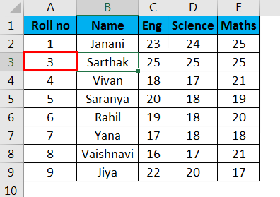
- Enter 1 in the A2 cell and 2 in the A3 cell to make the pattern logical.
-
-
-
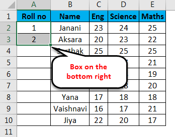
- There is a small black box on the bottom right of the selected cell.
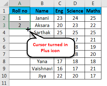
- The moment the cursor is kept on the cell, it changes to a plus icon.
-
-
-
- Drag the + symbol manually till the last cell of the range or double click on the plus icon, i.e. fill handle; a number will appear automatically in serial order.
-
Note:
-
-
- The row number will get updated in case of addition/deletion of row(s)
- It identifies the pattern of the series from the two filled cells and fills the rest of the cells.
- This method does not work on an empty row.
- Numbers are listed serially; however, the roman number format and alphabet listing are not considered.
- The serial number inserted is a static value.
-
2. Fill Series Method
This method is more controlled and systematic in numbering the rows.
Steps to be followed:
-
-
- Enter 1 in the A2 cell -> go to ‘Home tab of the ribbon.
-
-
-
- Select “Fill”drop-down -> Series
-
-
-
- Series dialog box will appear.
-
-
-
- Click the Columns button under Series and insert number 9 in the Stop value: input box. Press OK. The number series will appear.
-
Fill the first cell and apply the below steps.
-
-
- This method works on an empty row also.
- Numbers are listed serially, but the roman number and alphabets listing are not considered.
- The serial number inserted is a static value. A serial number does not change automatically.
-
3. COUNTA function Method
The COUNTA function is used in numbering only those rows that are not empty within a range.
Steps to be followed:
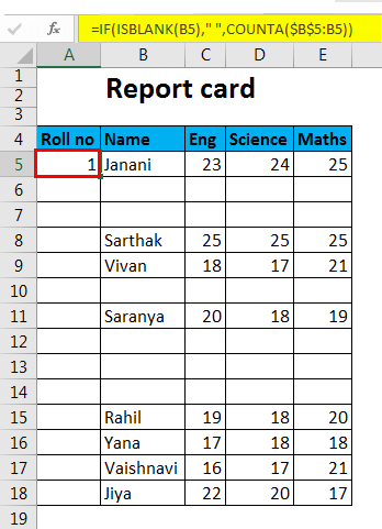
Select the cell A5, corresponding to the first non-empty row in the range and paste the following formula –
=IF(ISBLANK(B5),” “,COUNTA($B$5:B5))
Then, the cell gets populated with the number 1. Then drag the fill handle (+) to the last cell within the column range.
-
-
- The number in a cell is dynamic in nature. When a row is deleted, existing serial numbers are automatically updated, serially.
- Blank rows are not considered.
-
4. Row function method
The Row function can be used to get the row numbering.
Follow the below process.
Enter the ROW() function and subtract 1 from it to assign the correct row number. ROW() calculates to 2; however, we want to set the cell value to 1, being the first row of the range; hence 1 is subtracted. Hence formula will be,
=ROW()-1
If the row starts from 5th, the formula will change accordingly, i.e. =ROW() – 4
-
-
- The row number will get updated in case of the addition/deletion of row(s).
- It is not referencing any cell in the formula and will automatically adjust the row number.
- It will display the row number even if the row is blank.
-
5. SUBTOTAL For Filtered Data
The SUBTOTAL function in Excel helps in the serial numbering of a filtered dataset copied into another datasheet.
Steps to be followed:
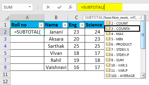
Here is a dataset which we intend to filter for marks in Maths greater than or equal to 20.
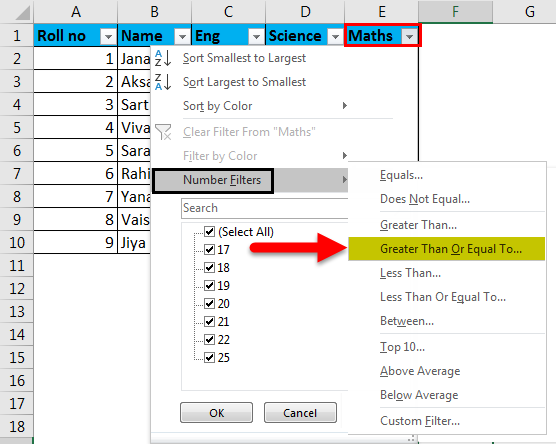
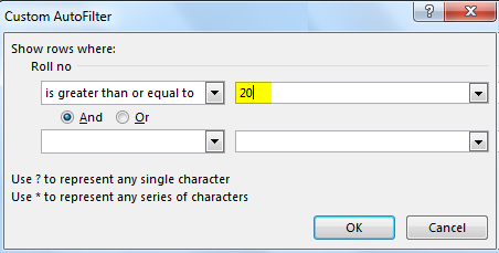
Now we will copy this filtered data into another sheet and delete the “Roll no” serial values.
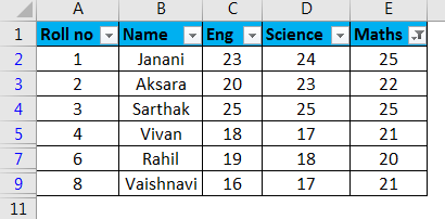
Then, select the first cell of the column range and use the ‘SUBTOTAL’ function wherein the first argument is 3, denoting ‘COUNT A’.
=SUBTOTAL(3,$B$2:B2)
This will populate the cell with a value of 1.
Now, with the selected cell, drag the fill handle (+) downwards along the column. This will populate the rest of the cells serially.
-
-
- The SUBTOTAL function is useful in rearranging the row count, serially, of a copied filtered dataset in another sheet.
- The serial numbers are automatically adjusted on the addition/deletion of rows.
-
6. By creating an Excel Table
Here, tabular data is converted into the Excel table.
Steps to be followed:
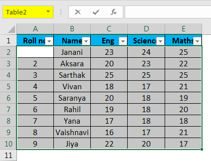
Firstly, select the whole dataset ->go to Insert Tab->Click on Table icon(CTRL+T) under Table group
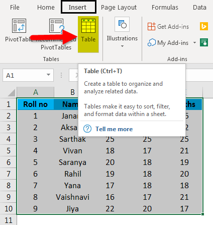
Create Table dialog box will appear. Specify range or table name
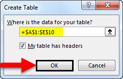
or
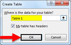
Click OK.
Tabular data is converted into Excel Table (named as Table 3).
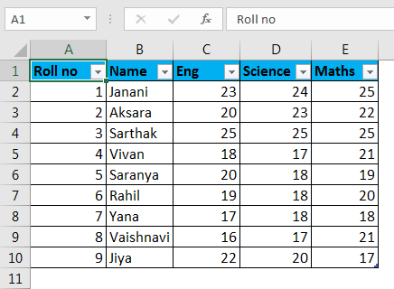
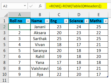
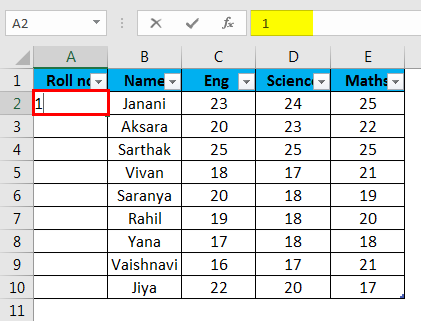
In the A2 cell, enter the formula.
Formula:
=Row()-Row(Table[#Header])
This will automatically fill the formula in all the cells.
-
-
- Row numbering will automatically adjust and update on the addition/deletion of rows.
-
7. By adding one to the previous row number
Subsequent rows get incremented by 1.
Steps to be followed:
As seen in the attached screenshot, enter 1 in cell A2 of the first row.
-
-
- Enter =A2+1 in cell A3
-
-
-
- Select A3 and drag the fill handle (+) to the last cell within the range. This will auto-populate the remaining cells.
-
-
-
- The cell value is relative to the previous cell value.
- Does not update serial number automatically on addition/deletion of rows.
-
Things to Remember about Auto Numbering in Excel
-
-
- The best way for auto numbering in excel depends on the type of data set you to have to enable.
- Auto Numbering in Excel is not an inbuilt function.
- Ensure to check if the Fill option is enabled for Auto Numbering in Excel.
-
Conclusion
There are different ways for Auto Numbering in Excel and number rows in serial order in excel. Some of the methods will do static numbering, whereas others would do dynamic updates on the addition/deletion of rows.
You can download this Auto Numbering Excel Excel Template here – Auto Numbering Excel Template.
Recommended Articles
This has been a guide to Auto Numbering in Excel. Here we discuss how to use Auto Numbering in Excel and Methods to number rows in Excel along with practical examples and downloadable excel template. You can also go through our other suggested articles –
-
- Excel Autofit
- Number Format In Excel
- Auto Format in Excel
- Numbering in Excel

on
November 25, 2010, 12:38 AM PST
A dynamic line-numbering formula for Excel
Use this formula to automatically number rows with data, especially if you anticipate lots of change.
Sometimes you need a solution to an uncommon problem, like numbering Excel lines. It isn’t a very Excel-like task, but I recently heard from someone that insisted that’s exactly what they needed. Why not just use the fill handle I asked. A dynamic list was needed—one that could accommodate change and blank rows. Here’s what I used:
=IF(cell<>"",COUNTA(cell:cell))As you can see in the following figure, this formula works well. If you insert or delete a row, the numbers update accordingly—almost. There’s a problem in row 9; if the row is empty, the formula returns FALSE. On the other hand, row 11 displays the formula’s flexibility. After deleting a row (ID 5), the formula updates as required. (I purposely left the ID column so you could see these changes.)
The FALSE value is easy to eliminate by updating the IF() function:
=IF(cell<>"",COUNTA(cell:cell),"")Add any required punctuation to the IF() function as well. If you concatenate the punctuation using the following form, Excel will display the punctuation for empty rows.
=IF(cell<>"",COUNTA(cell:cell),"") & "."
Instead, add the punctuation to the IF() function as follows:
=IF(cell<>"",COUNTA(cell:cell) & ".","")Although this formula works and seems to accommodate all the possibilities, I’m still not convinced it’s the most efficient solution–do you have a better one? I’d also like to know if anyone has a use for such a formula. How might you use it?
-
Software