
-
Select the cell where you want the result to appear.
-
On the Formulas tab, click More Functions, point to Statistical, and then click one of the following functions:
-
COUNTA: To count cells that are not empty
-
COUNT: To count cells that contain numbers.
-
COUNTBLANK: To count cells that are blank.
-
COUNTIF: To count cells that meets a specified criteria.
Tip: To enter more than one criterion, use the COUNTIFS function instead.
-
-
Select the range of cells that you want, and then press RETURN.
-
Select the cell where you want the result to appear.
-
On the Formulas tab, click Insert, point to Statistical, and then click one of the following functions:
-
COUNTA: To count cells that are not empty
-
COUNT: To count cells that contain numbers.
-
COUNTBLANK: To count cells that are blank.
-
COUNTIF: To count cells that meets a specified criteria.
Tip: To enter more than one criterion, use the COUNTIFS function instead.
-
-
Select the range of cells that you want, and then press RETURN.
Содержание
- Auto-Numbering in Excel – How to Number Cells Automatically
- How to Auto-Number Cells with a Regular Pattern
- How to Auto-Number Cells Using the ROW() Function
- Conclusion
- Принципы нумерации ячеек в Microsoft Excel
- Виды нумерации в Microsoft Excel
- Способ 1: переключение режима нумерации
- Способ 2: маркер заполнения
- Способ 3: прогрессия
- Способ 4: использование функции
- Способ 5: присвоение имени ячейке
Auto-Numbering in Excel – How to Number Cells Automatically

Numbering cells is a task often you’ll often perform in Excel. But writing the number manually in each cell takes a lot of time.
Fortunately, there are methods that help you add numbers automatically. And in this article, I’ll show you two methods of doing so: the first is a simple method, and the second lets you have dynamically numbered cells. So let’s get started.
How to Auto-Number Cells with a Regular Pattern
For this method, you set your starting number in one cell and the next number in the series in the next cell.
Once you have two adjacent cells filled with your two starting numbers, you can select those two cells, click on the handle in the bottom right corner of the green outline, and drag to select all the cells that you want to follow your pattern.
A useful tooltip appears near the bottom right corner of the green outline to show what the last number in the series would be if you released at that point.
So, if you want to start with the number 5 and increment by 3 until 38, you would write 5 in your first cell, and 8 in the next cell. You would then select the cells containing the 5 and the 8, click on the handle, and drag to select the other cells until you see 38 appear in the tooltip. Then you can release, and the numbers will be filled in automatically.
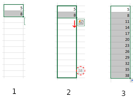 1) Select the cells. 2) Drag the handle on the outline (you can also see the tooltip with the last number in the series) 3) Release
The numbers can also be formatted in descending order: if you start with 7 and then enter 5, the pattern will continue with 3, 1, -1, and so on.
You can also do the same with rows instead of columns. Fill in two consecutive cells in a row with the start of your pattern, then select them and drag the outline horizontally across those cells that you want to continue that pattern. It’ll automatically fill in those numbers.
You can also do the same going upward – fill two cells, select them, click the handle and drag upward to fill the cells above your two starting cells.
Note: this will always add numbers that are evenly spaced in the pattern you’ve started. It won’t work with other kinds of number progressions.
How to Auto-Number Cells Using the ROW() Function
If you have data that can be sorted in different ways (say, a list of names — alphabetically, etc), it’s annoying if the numbering of your lines gets scrambled when you’re sorting other data.
To avoid that, you can dynamically number your rows using the ROW() function.
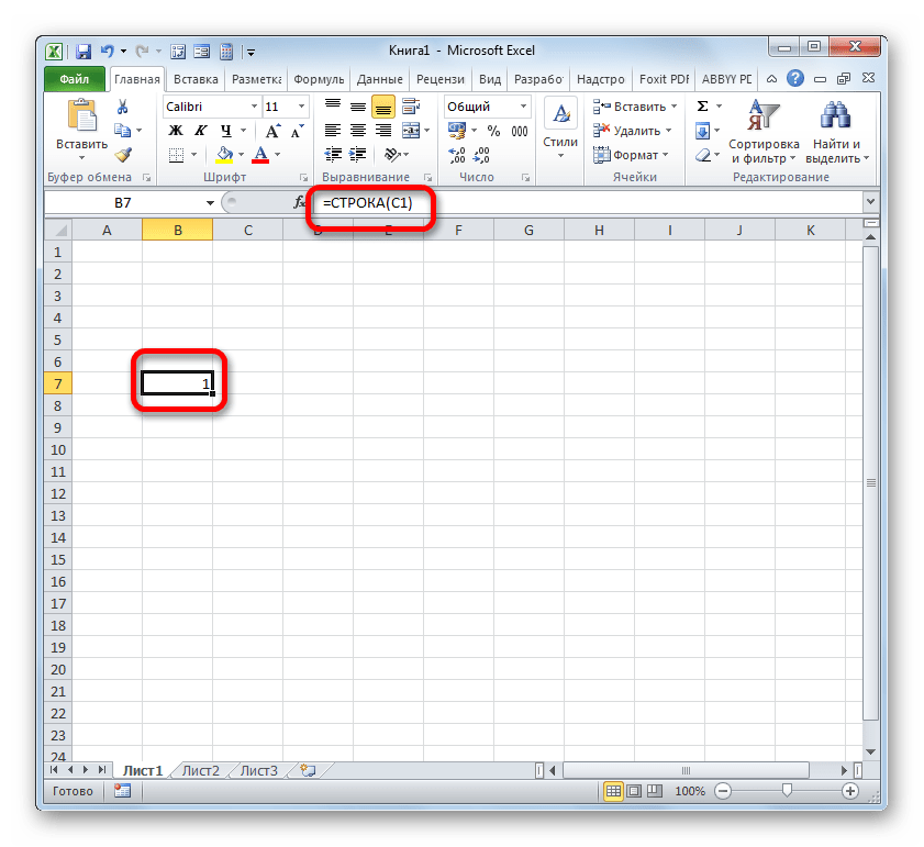
In the cell where you want the numbering to start, write =ROW(A1) . This will produce the number 1 in the cell.
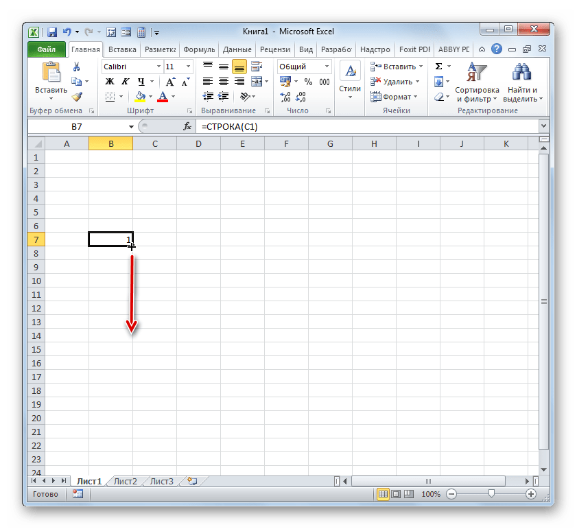
Select the cell and drag the outline from the handle in the corner to populate the same formula in the rest of the cells (or, if you are adding the line numbers near a block of data already present, you can just double-click on the handle on the corner of the selection).
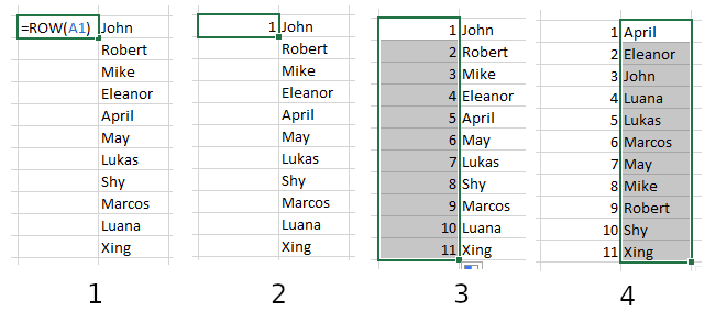 1) Write =ROW(A1) in your first cell, 2) It will appear as the number 1 , 3) Click and drag or double-click to fill all other cells. 4) Now if you sort the data, the line numbers will stay in order.
If you want to have a different regular pattern, you can use a bit of math: to have numbers spaced by 2, you can write =ROW(A1) * 2 in the first cell, and then proceed with the same steps as above. This will produce the numbers 2, 4, 6. and so on.
If you want to change the starting point of the pattern – to maybe have only odd numbers, for example – you can subtract one: =ROW(A1) * 2 — 1 , this will produce the numbers 1, 3, 5, 7.
As a general formula, to get any pattern you can write =ROW(A1) * a + b . a is used to determine the step, and b (it can be either a positive or negative number) is used to change the starting point of the pattern.
If you want to number your columns, you can use the COLUMN() function in the same way as the ROW() . Just fill in your first cell with =COLUMN(A1) , select the cell, then expand the selection to the rest of the cells you want your numbers to be in.
Note: if you add or delete rows, you will need to set the auto-numbering again by selecting the first cell and dragging or double-clicking again to restore the pattern.
Conclusion
Writing numbers in cells is a task often performed in Excel, and here we have seen two simple methods that let us save time. The first method just involves writing numbers in two cells, and then a couple of clicks. And the other just requires writing a formula in one cell, and then a couple of clicks.
There are a few other methods for numbering cells in Excel, but these are the most straightforward.
Источник
Принципы нумерации ячеек в Microsoft Excel

Для пользователей программы Microsoft Excel не секрет, что данные в этом табличном процессоре размещаются в отдельных ячейках. Для того, чтобы пользователь мог обращаться к этим данным, каждому элементу листа присвоен адрес. Давайте выясним, по какому принципу нумеруются объекты в Экселе и можно ли изменить данную нумерацию.
Виды нумерации в Microsoft Excel
Прежде всего, следует сказать о том, что в Экселе имеется возможность переключения между двумя видами нумерации. Адрес элементов при использовании первого варианта, который установлен по умолчанию, имеет вид A1. Второй вариант представлен следующей формой — R1C1. Для его использования требуется произвести переключение в настройках. Кроме того, пользователь может собственноручно пронумеровать ячейки, воспользовавшись сразу несколькими вариантами. Давайте рассмотрим все эти возможности подробнее.
Способ 1: переключение режима нумерации
Прежде всего, давайте рассмотрим возможность переключения режима нумерации. Как уже говорилось ранее, адрес ячеек по умолчанию задается по типу A1. То есть, столбцы обозначаются буквами латинского алфавита, а строчки – арабскими цифрами. Переключение в режим R1C1 предполагает вариант, при котором цифрами задаются не только координаты строк, но и столбцов. Давайте разберемся, как произвести такое переключение.
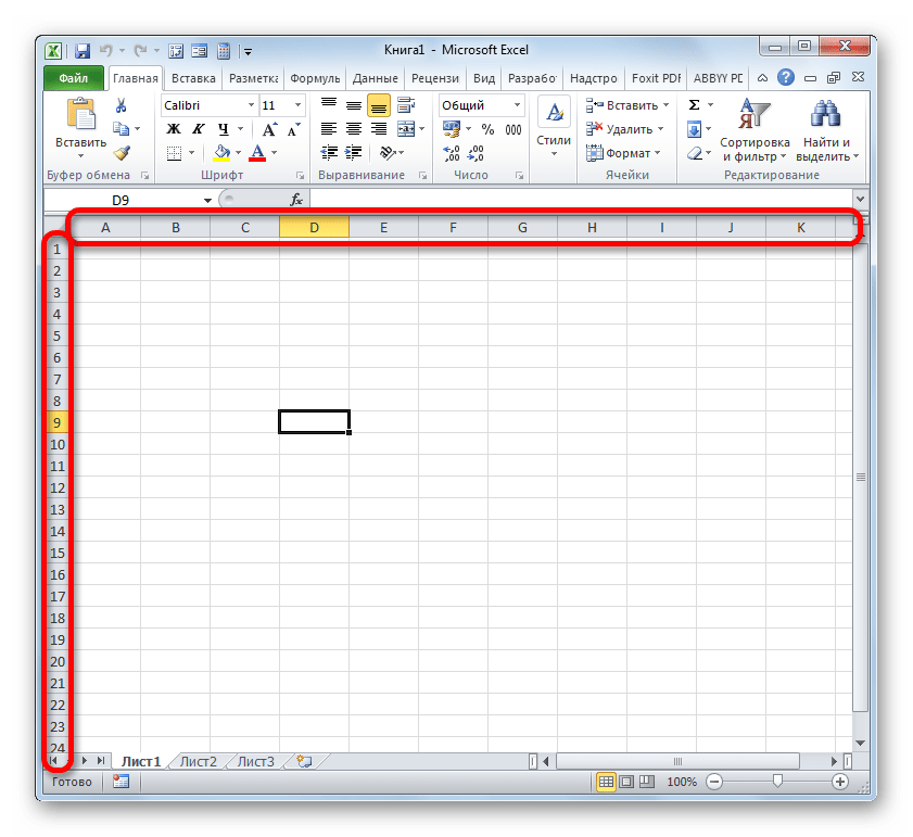
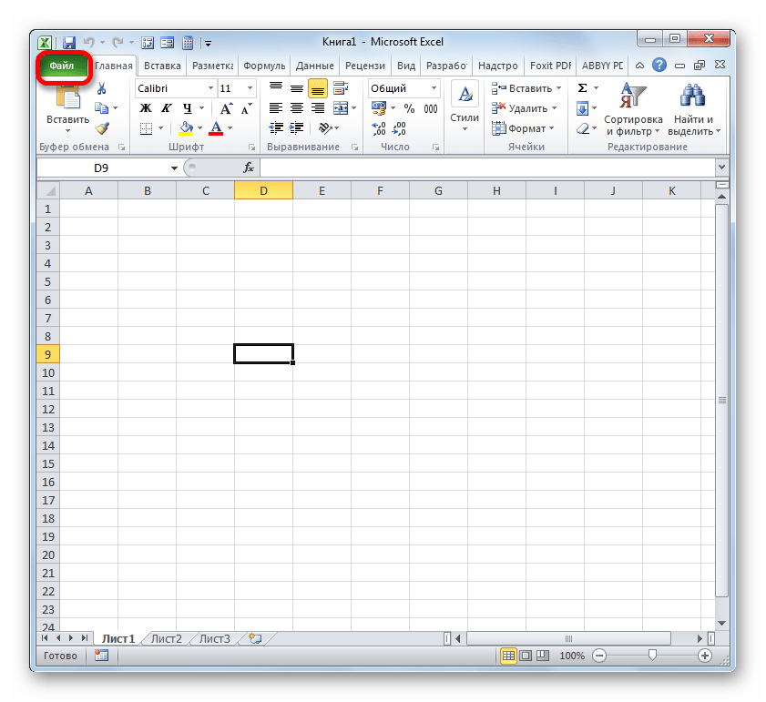
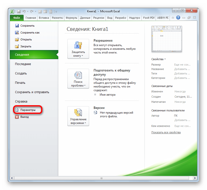
- Производим перемещение во вкладку «Файл».

- В открывшемся окне посредством левого вертикального меню переходим в раздел «Параметры».
Для того, чтобы вернуть обозначение координат по умолчанию, нужно провести ту же самую процедуру, только на этот раз снять флажок с пункта «Стиль ссылок R1C1».
Способ 2: маркер заполнения
Кроме того, пользователь сам может пронумеровать строки или столбцы, в которых расположены ячейки, согласно своим потребностям. Эта пользовательская нумерация может использоваться для обозначения строчек или колонок таблицы, для передачи номера строчки встроенным функциям Excel и в других целях. Конечно, нумерацию можно произвести вручную, просто вбивая с клавиатуры нужные числа, но намного проще и быстрее выполнить данную процедуру, используя инструменты автозаполнения. Особенно это актуально при нумерации большого массива данных.
Взглянем, как при помощи маркера заполнения можно произвести автонумерацию элементов листа.

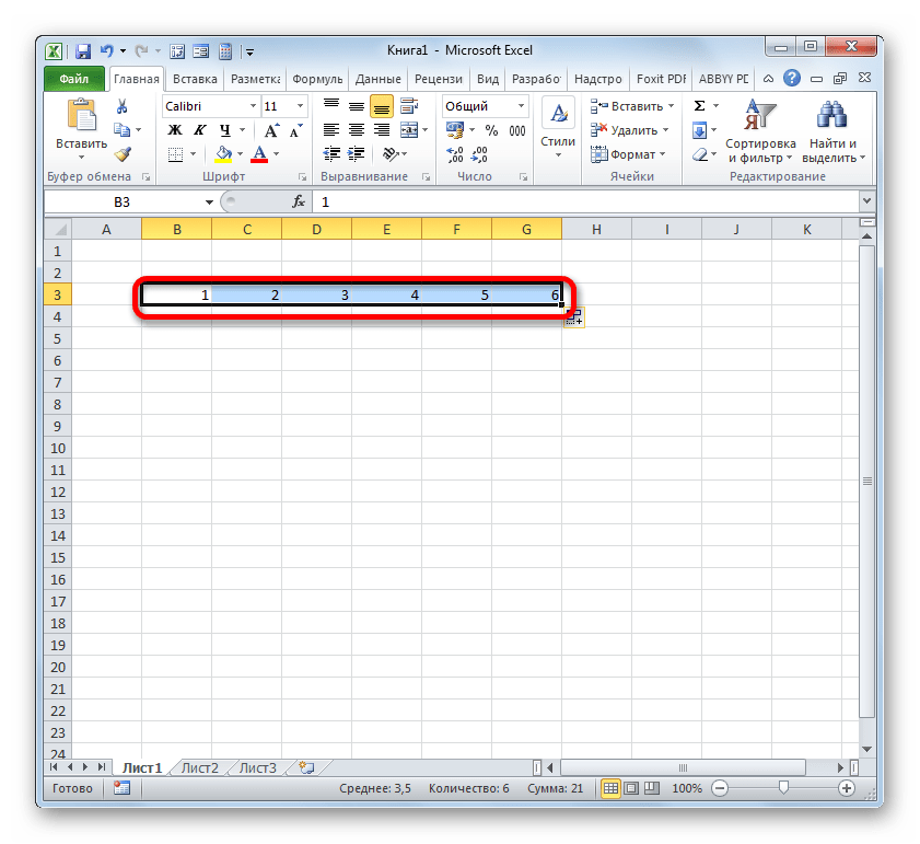
- Ставим цифру «1» в ту ячейку, с которой планируем начинать нумерацию. Затем наводим курсор на правый нижний край указанного элемента. При этом он должен трансформироваться в черный крестик. Он носит название маркера заполнения. Зажимаем левую кнопку мышки и тащим курсор вниз или вправо, в зависимости от того, что именно нужно пронумеровать: строчки или столбцы.
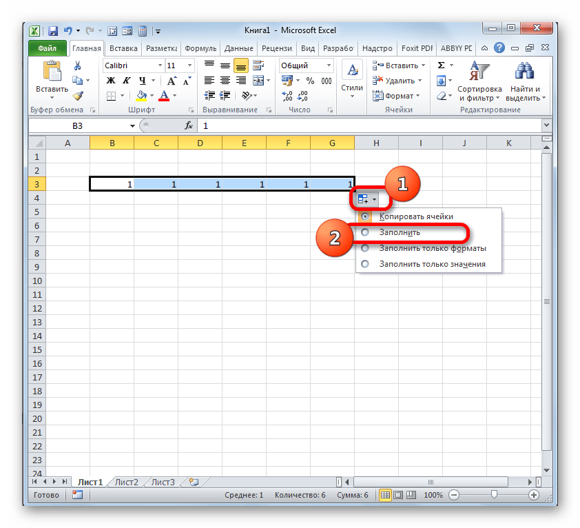
- После того, как достигли последней ячейки, которую следует пронумеровать, отпускаем кнопку мышки. Но, как видим, все элементы с нумерацией заполнены только лишь единицами. Для того, чтобы это исправить, жмем на пиктограмму, которая находится в конце нумерованного диапазона. Выставляем переключатель около пункта «Заполнить».
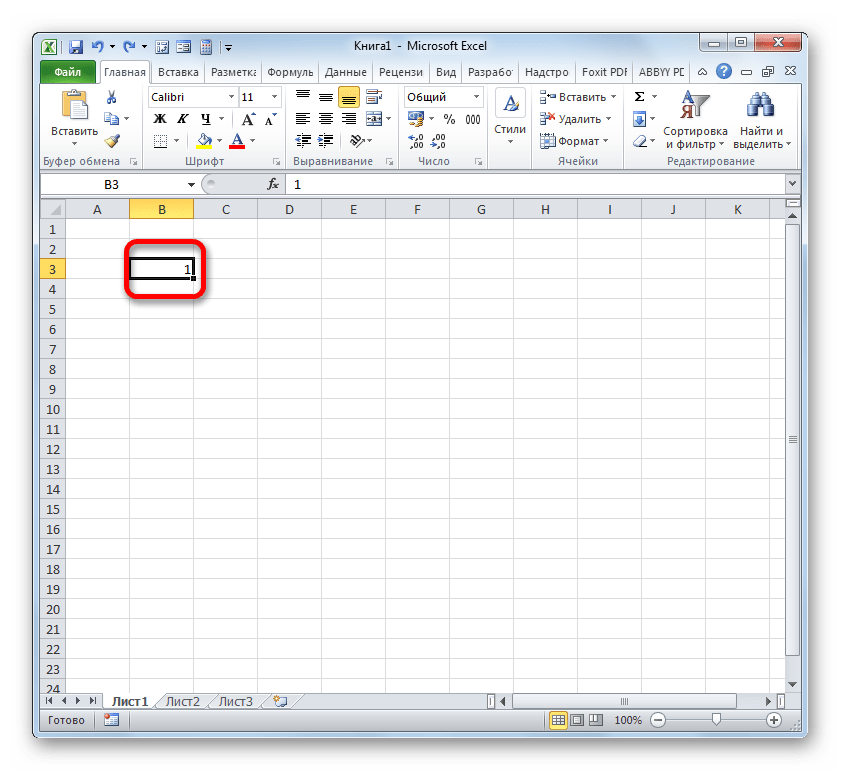
- После выполнения данного действия весь диапазон будет пронумерован по порядку.
Способ 3: прогрессия
Ещё одним способом, с помощью которого можно пронумеровать объекты в Экселе, является использование инструмента под названием «Прогрессия».
- Как и в предыдущем способе, устанавливаем цифру «1» в первую ячейку, подлежащую нумерации. После этого просто выделяем данный элемент листа, кликнув по нему левой кнопкой мыши.
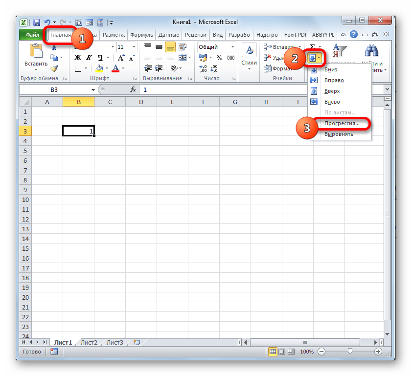
- После того, как нужный диапазон выделен, перемещаемся во вкладку «Главная». Кликаем по кнопке «Заполнить», размещенной на ленте в блоке «Редактирование». Открывается список действий. Выбираем из него позицию «Прогрессия…».
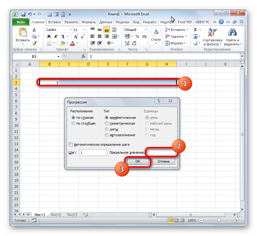
- Открывается окно Excel под названием «Прогрессия». В этом окне множество настроек. Прежде всего, остановимся на блоке «Расположение». В нём переключатель имеет две позиции: «По строкам» и «По столбцам». Если вам нужно произвести горизонтальную нумерацию, то выбирайте вариант «По строкам», если вертикальную – то «По столбцам».
В блоке настроек «Тип» для наших целей нужно установить переключатель в позицию «Арифметическая». Впрочем, он и так по умолчанию расположен в данной позиции, поэтому нужно лишь проконтролировать его положение.
Блок настроек «Единицы» становится активным только при выборе типа «Даты». Так как мы выбрали тип «Арифметическая», нас вышеуказанный блок интересовать не будет.
В поле «Шаг» следует установить цифру «1». В поле «Предельное значение» ставим количество нумеруемых объектов.
После выполнения перечисленных действий жмем на кнопку «OK» внизу окошка «Прогрессия». 

Если вы не желаете производить подсчет количества элементов листа, которые нужно пронумеровать, чтобы указать их в поле «Предельное значение» в окне «Прогрессия», то в этом случае нужно перед запуском указанного окна выделить весь диапазон, подлежащий нумерации.

После этого в окне «Прогрессия» выполняем все те же действия, которые были описаны выше, но на этот раз оставляем поле «Предельное значение» пустым.
Результат будет тот же: выделенные объекты окажутся пронумерованными.
Способ 4: использование функции
Пронумеровать элементы листа, можно также прибегнув к использованию встроенных функций Excel. Например, для построчной нумерации можно применять оператор СТРОКА.
Функция СТРОКА относится к блоку операторов «Ссылки и массивы». Её основной задачей является возврат номера строчки листа Excel, на который будет установлена ссылка. То есть, если мы укажем в качестве аргумента этой функции любую ячейку в первой строке листа, то она выведет значение «1» в ту ячейку, где располагается сама. Если указать ссылку на элемент второй строчки, то оператор выведет цифру «2» и т.д.
Синтаксис функции СТРОКА следующий:
Как видим, единственным аргументом данной функции является ссылка на ячейку, номер строки которой нужно вывести в указанный элемент листа.
Посмотрим, как работать с указанным оператором на практике.
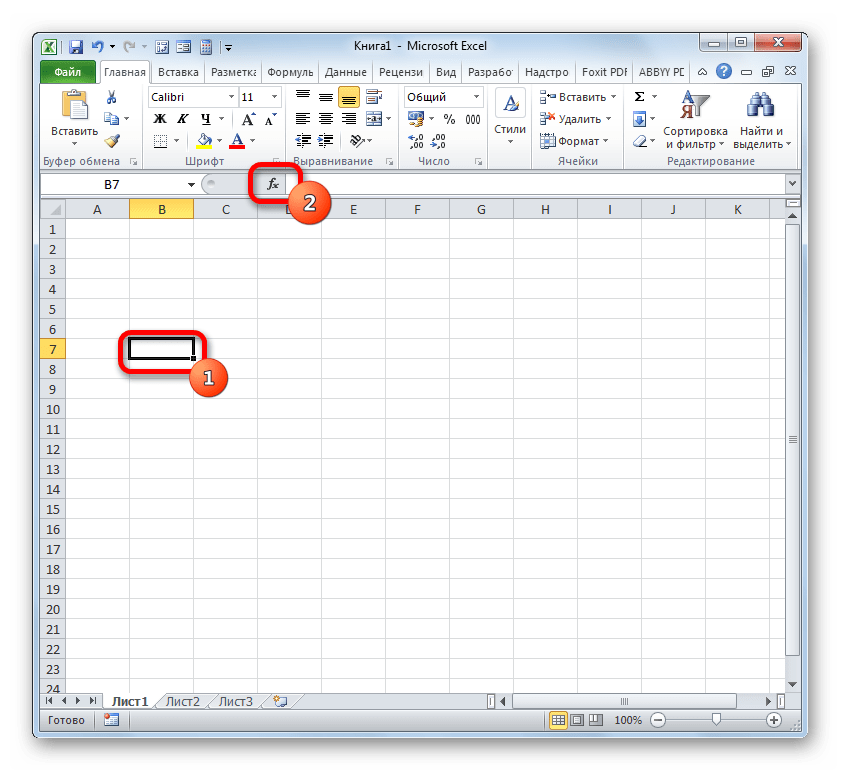
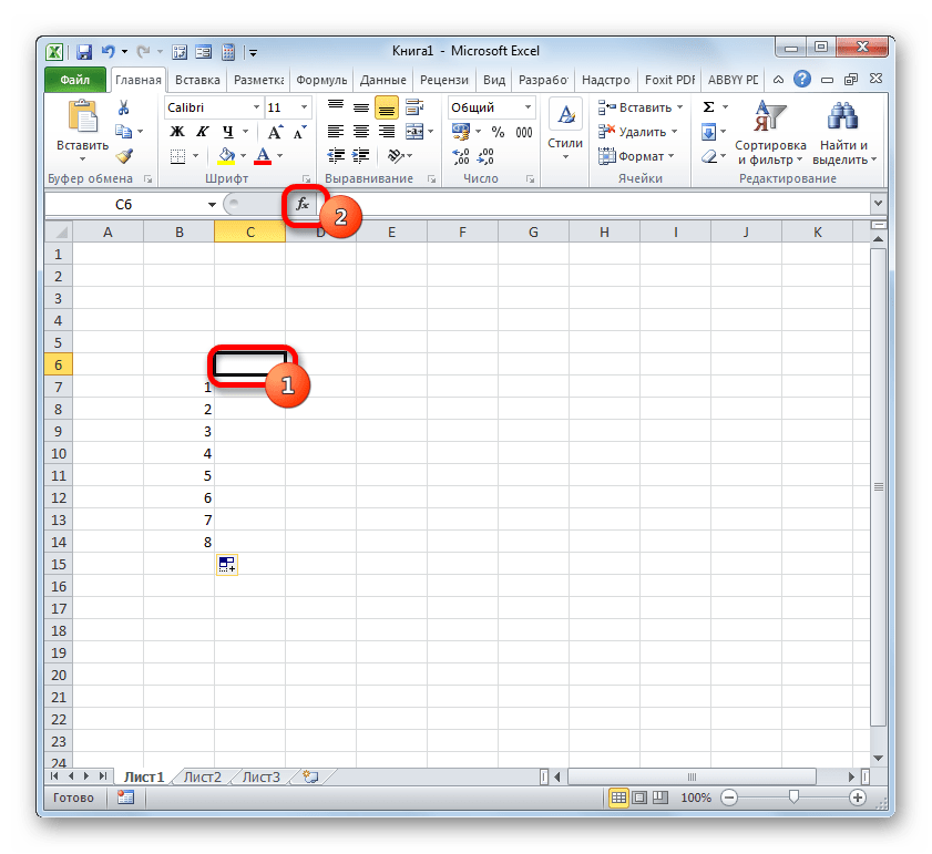
- Выделяем объект, который будет первым в нумерованном диапазоне. Щелкаем по значку «Вставить функцию», который размещен над рабочей областью листа Excel.
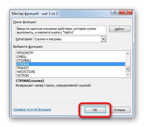
- Запускается Мастер функций. Делаем переход в нем в категорию «Ссылки и массивы». Из перечисленных названий операторов выбираем наименование «СТРОКА». После выделения данного названия клацаем по кнопке «OK».
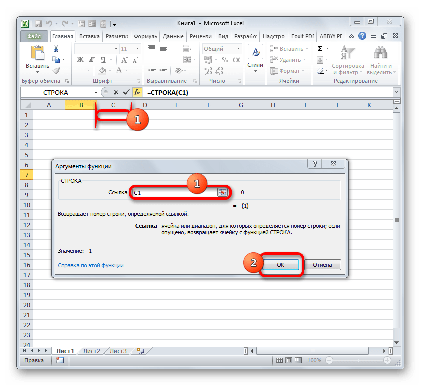
- Запускает окно аргументов функции СТРОКА. Оно имеет всего одно поле, по числу этих самых аргументов. В поле «Ссылка» нам требуется ввести адрес любой ячейки, которая расположена в первой строчке листа. Координаты можно ввести вручную, вбив их посредством клавиатуры. Но все-таки более удобно это сделать, просто установив курсор в поле, а затем клацнув левой кнопкой мыши по любому элементу в первой строке листа. Её адрес тут же будет выведен в окне аргументов СТРОКА. Затем жмем на кнопку «OK».
- В той ячейке листа, в которой расположилась функция СТРОКА, отобразилась цифра «1».
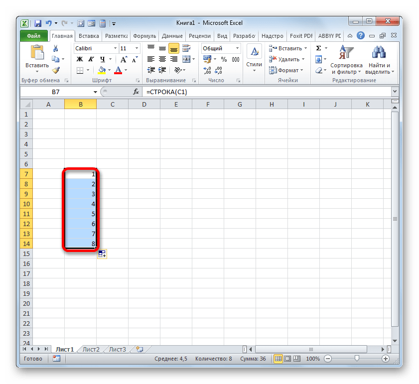
- Теперь нам нужно пронумеровать все остальные строки. Для того, чтобы не производить процедуру с использованием оператора для всех элементов, что, безусловно, займет много времени, произведем копирование формулы посредством уже знакомого нам маркера заполнения. Наводим курсор на нижний правый край ячейки с формулой СТРОКА и после появления маркера заполнения зажимаем левую кнопку мышки. Протягиваем курсор вниз на то количество строчек, которое нужно пронумеровать.
- Как видим, после выполнения данного действия все строки указанного диапазона будут пронумерованы пользовательской нумерацией.
Но мы совершили нумерацию только строк, а для полноценного выполнения задачи присвоения адреса ячейки в виде номера внутри таблицы следует пронумеровать ещё и столбцы. Это также можно сделать при помощи встроенной функции Excel. Данный оператор ожидаемо имеет наименование «СТОЛБЕЦ».
Функция СТОЛБЕЦ также относится к категории операторов «Ссылки и массивы». Как нетрудно догадаться её задачей является выведение в указанный элемент листа номера столбца, на ячейку которого дается ссылка. Синтаксис этой функции практически идентичен предыдущему оператору:
Как видим, отличается только наименование самого оператора, а аргументом, как и в прошлый раз, остается ссылка на конкретный элемент листа.
Посмотрим, как выполнить поставленную задачу с помощью данного инструмента на практике.
- Выделяем объект, которому будет соответствовать первый столбец обрабатываемого диапазона. Клацаем по пиктограмме «Вставить функцию».
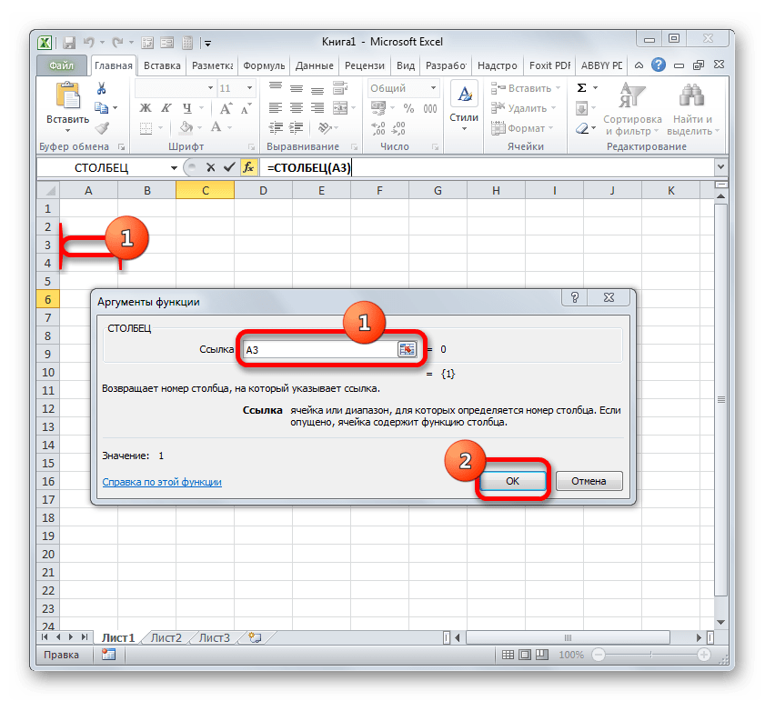
- Прейдя в Мастер функций, перемещаемся в категорию «Ссылки и массивы» и там выделяем наименование «СТОЛБЕЦ». Клацаем по кнопке «OK».
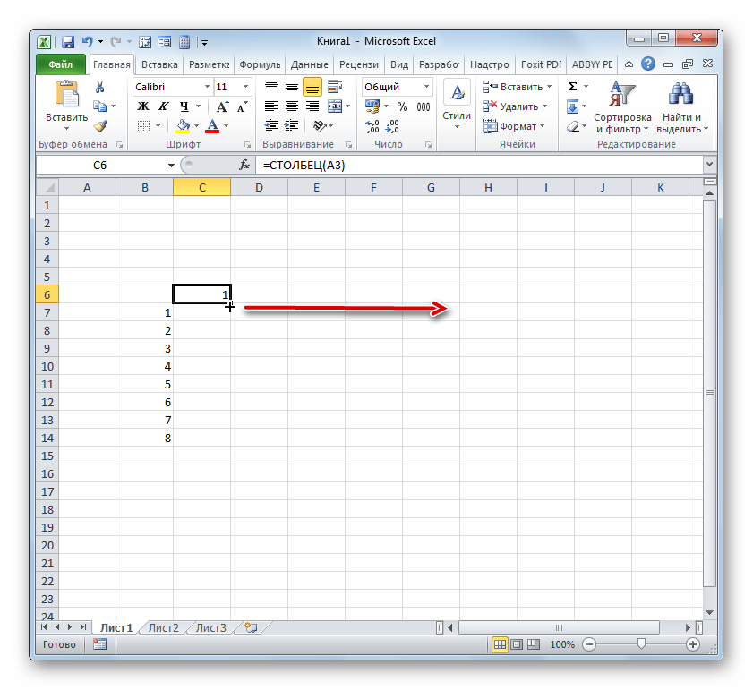
- Происходит запуск окна аргументов СТОЛБЕЦ. Как и в предыдущий раз, ставим курсор в поле «Ссылка». Но в этом случае выделяем любой элемент не первой строки листа, а первого столбца. Координаты тут же отобразятся в поле. Затем можно клацать по кнопке «OK».
- После этого в указанную ячейку будет выведена цифра «1», соответствующая относительному номеру столбца таблицы, который задан пользователем. Для нумерации остальных столбцов, так же, как и в случае со строками, применим маркер заполнения. Наводим курсор на нижний правый край ячейки, содержащей функцию СТОЛБЕЦ. Дожидаемся появления маркера заполнения и, зажав левую кнопку мыши, тащим курсор вправо на нужное количество элементов.
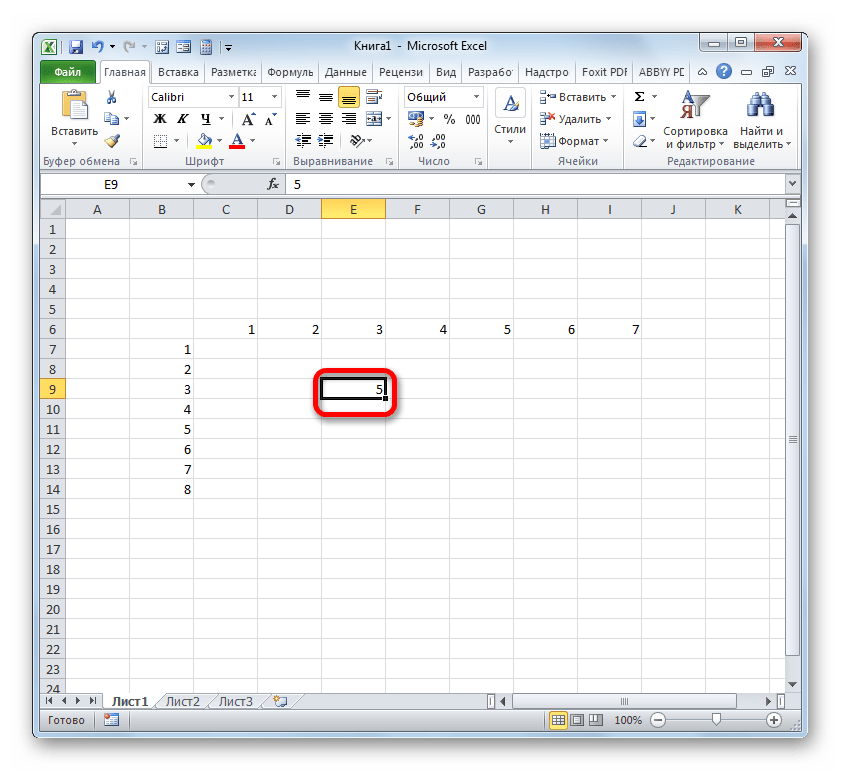
Теперь все ячейки нашей условной таблицы имеют свою относительную нумерацию. Например, элемент, в котором на изображении ниже установлена цифра 5, имеет относительные пользовательские координаты (3;3), хотя абсолютный его адрес в контексте листа остаётся E9.
Способ 5: присвоение имени ячейке
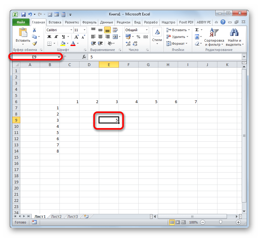
В дополнение к вышеуказанным способам нужно отметить, что, несмотря на проведенное присвоения номеров столбцам и строкам определенного массива, наименования ячеек внутри него будут задаваться в соответствии с нумерацией листа в целом. Это можно увидеть в специальном поле имен при выделении элемента.
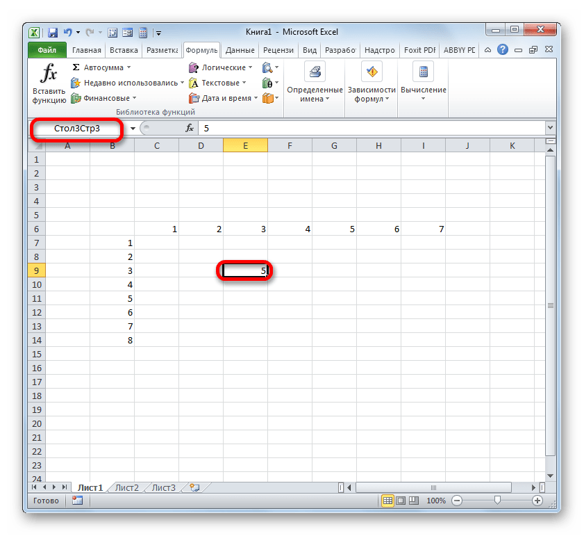
Для того, чтобы изменить имя, соответствующее координатам листа на то, которое мы задали с помощью относительных координат для нашего массива, достаточно выделить соответствующий элемент кликом левой кнопки мыши. Затем просто с клавиатуры в поле имени вбить то название, которое пользователь считает нужным. Это может быть любое слово. Но в нашем случае мы просто введем относительные координаты данного элемента. В нашем наименовании обозначим номер строки буквами «Стр», а номер столбца «Стол». Получаем наименование следующего типа: «Стол3Стр3». Вбиваем его в поле имен и жмем на клавишу Enter.
Теперь нашей ячейке присвоено наименование согласно её относительному адресу в составе массива. Таким же образом можно дать имена и другим элементам массива.
Как видим, существуют два вида встроенной нумерации в Экселе: A1 (по умолчанию) и R1C1 (включается в настройках). Данные виды адресации распространяются на весь лист в целом. Но кроме того, каждый пользователь может сделать свою пользовательскую нумерацию внутри таблицы или определенного массива данных. Существует несколько проверенных способов присвоения ячейкам пользовательских номеров: с помощью маркера заполнения, инструмента «Прогрессия» и специальных встроенных функций Excel. После того, как выставлена нумерация, можно на её основе присвоить имя конкретному элементу листа.
Источник
Содержание
- Виды нумерации в Microsoft Excel
- Способ 1: переключение режима нумерации
- Способ 2: маркер заполнения
- Способ 3: прогрессия
- Способ 4: использование функции
- Способ 5: присвоение имени ячейке
- Вопросы и ответы
Для пользователей программы Microsoft Excel не секрет, что данные в этом табличном процессоре размещаются в отдельных ячейках. Для того, чтобы пользователь мог обращаться к этим данным, каждому элементу листа присвоен адрес. Давайте выясним, по какому принципу нумеруются объекты в Экселе и можно ли изменить данную нумерацию.
Виды нумерации в Microsoft Excel
Прежде всего, следует сказать о том, что в Экселе имеется возможность переключения между двумя видами нумерации. Адрес элементов при использовании первого варианта, который установлен по умолчанию, имеет вид A1. Второй вариант представлен следующей формой — R1C1. Для его использования требуется произвести переключение в настройках. Кроме того, пользователь может собственноручно пронумеровать ячейки, воспользовавшись сразу несколькими вариантами. Давайте рассмотрим все эти возможности подробнее.
Способ 1: переключение режима нумерации
Прежде всего, давайте рассмотрим возможность переключения режима нумерации. Как уже говорилось ранее, адрес ячеек по умолчанию задается по типу A1. То есть, столбцы обозначаются буквами латинского алфавита, а строчки – арабскими цифрами. Переключение в режим R1C1 предполагает вариант, при котором цифрами задаются не только координаты строк, но и столбцов. Давайте разберемся, как произвести такое переключение.
- Производим перемещение во вкладку «Файл».
- В открывшемся окне посредством левого вертикального меню переходим в раздел «Параметры».
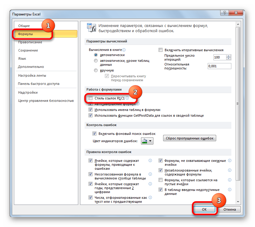
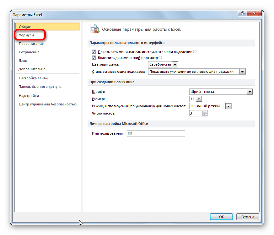
- Открывается окно параметров Эксель. Через меню, которое размещено слева, переходим в подраздел «Формулы».
- После перехода обращаем внимание на правую часть окна. Ищем там группу настроек «Работа с формулами». Около параметра «Стиль ссылок R1C1» ставим флажок. После этого можно жать на кнопку «OK» в нижней части окна.
- После названных выше манипуляций в окне параметров стиль ссылок поменяется на R1C1. Теперь не только строчки, но и столбцы будут нумероваться цифрами.


Для того, чтобы вернуть обозначение координат по умолчанию, нужно провести ту же самую процедуру, только на этот раз снять флажок с пункта «Стиль ссылок R1C1».
Урок: Почему в Экселе вместо букв цифры
Способ 2: маркер заполнения
Кроме того, пользователь сам может пронумеровать строки или столбцы, в которых расположены ячейки, согласно своим потребностям. Эта пользовательская нумерация может использоваться для обозначения строчек или колонок таблицы, для передачи номера строчки встроенным функциям Excel и в других целях. Конечно, нумерацию можно произвести вручную, просто вбивая с клавиатуры нужные числа, но намного проще и быстрее выполнить данную процедуру, используя инструменты автозаполнения. Особенно это актуально при нумерации большого массива данных.
Взглянем, как при помощи маркера заполнения можно произвести автонумерацию элементов листа.
- Ставим цифру «1» в ту ячейку, с которой планируем начинать нумерацию. Затем наводим курсор на правый нижний край указанного элемента. При этом он должен трансформироваться в черный крестик. Он носит название маркера заполнения. Зажимаем левую кнопку мышки и тащим курсор вниз или вправо, в зависимости от того, что именно нужно пронумеровать: строчки или столбцы.
- После того, как достигли последней ячейки, которую следует пронумеровать, отпускаем кнопку мышки. Но, как видим, все элементы с нумерацией заполнены только лишь единицами. Для того, чтобы это исправить, жмем на пиктограмму, которая находится в конце нумерованного диапазона. Выставляем переключатель около пункта «Заполнить».
- После выполнения данного действия весь диапазон будет пронумерован по порядку.

Способ 3: прогрессия
Ещё одним способом, с помощью которого можно пронумеровать объекты в Экселе, является использование инструмента под названием «Прогрессия».
- Как и в предыдущем способе, устанавливаем цифру «1» в первую ячейку, подлежащую нумерации. После этого просто выделяем данный элемент листа, кликнув по нему левой кнопкой мыши.
- После того, как нужный диапазон выделен, перемещаемся во вкладку «Главная». Кликаем по кнопке «Заполнить», размещенной на ленте в блоке «Редактирование». Открывается список действий. Выбираем из него позицию «Прогрессия…».
- Открывается окно Excel под названием «Прогрессия». В этом окне множество настроек. Прежде всего, остановимся на блоке «Расположение». В нём переключатель имеет две позиции: «По строкам» и «По столбцам». Если вам нужно произвести горизонтальную нумерацию, то выбирайте вариант «По строкам», если вертикальную – то «По столбцам».
В блоке настроек «Тип» для наших целей нужно установить переключатель в позицию «Арифметическая». Впрочем, он и так по умолчанию расположен в данной позиции, поэтому нужно лишь проконтролировать его положение.
Блок настроек «Единицы» становится активным только при выборе типа «Даты». Так как мы выбрали тип «Арифметическая», нас вышеуказанный блок интересовать не будет.
В поле «Шаг» следует установить цифру «1». В поле «Предельное значение» ставим количество нумеруемых объектов.
После выполнения перечисленных действий жмем на кнопку «OK» внизу окошка «Прогрессия».
- Как видим, указанный в окне «Прогрессия» диапазон элементов листа будет пронумерован по порядку.
Если вы не желаете производить подсчет количества элементов листа, которые нужно пронумеровать, чтобы указать их в поле «Предельное значение» в окне «Прогрессия», то в этом случае нужно перед запуском указанного окна выделить весь диапазон, подлежащий нумерации.
После этого в окне «Прогрессия» выполняем все те же действия, которые были описаны выше, но на этот раз оставляем поле «Предельное значение» пустым.
Результат будет тот же: выделенные объекты окажутся пронумерованными.
Урок: Как сделать автозаполнение в Экселе
Способ 4: использование функции
Пронумеровать элементы листа, можно также прибегнув к использованию встроенных функций Excel. Например, для построчной нумерации можно применять оператор СТРОКА.
Функция СТРОКА относится к блоку операторов «Ссылки и массивы». Её основной задачей является возврат номера строчки листа Excel, на который будет установлена ссылка. То есть, если мы укажем в качестве аргумента этой функции любую ячейку в первой строке листа, то она выведет значение «1» в ту ячейку, где располагается сама. Если указать ссылку на элемент второй строчки, то оператор выведет цифру «2» и т.д.
Синтаксис функции СТРОКА следующий:
=СТРОКА(ссылка)
Как видим, единственным аргументом данной функции является ссылка на ячейку, номер строки которой нужно вывести в указанный элемент листа.
Посмотрим, как работать с указанным оператором на практике.
- Выделяем объект, который будет первым в нумерованном диапазоне. Щелкаем по значку «Вставить функцию», который размещен над рабочей областью листа Excel.
- Запускается Мастер функций. Делаем переход в нем в категорию «Ссылки и массивы». Из перечисленных названий операторов выбираем наименование «СТРОКА». После выделения данного названия клацаем по кнопке «OK».
- Запускает окно аргументов функции СТРОКА. Оно имеет всего одно поле, по числу этих самых аргументов. В поле «Ссылка» нам требуется ввести адрес любой ячейки, которая расположена в первой строчке листа. Координаты можно ввести вручную, вбив их посредством клавиатуры. Но все-таки более удобно это сделать, просто установив курсор в поле, а затем клацнув левой кнопкой мыши по любому элементу в первой строке листа. Её адрес тут же будет выведен в окне аргументов СТРОКА. Затем жмем на кнопку «OK».
- В той ячейке листа, в которой расположилась функция СТРОКА, отобразилась цифра «1».
- Теперь нам нужно пронумеровать все остальные строки. Для того, чтобы не производить процедуру с использованием оператора для всех элементов, что, безусловно, займет много времени, произведем копирование формулы посредством уже знакомого нам маркера заполнения. Наводим курсор на нижний правый край ячейки с формулой СТРОКА и после появления маркера заполнения зажимаем левую кнопку мышки. Протягиваем курсор вниз на то количество строчек, которое нужно пронумеровать.
- Как видим, после выполнения данного действия все строки указанного диапазона будут пронумерованы пользовательской нумерацией.
Но мы совершили нумерацию только строк, а для полноценного выполнения задачи присвоения адреса ячейки в виде номера внутри таблицы следует пронумеровать ещё и столбцы. Это также можно сделать при помощи встроенной функции Excel. Данный оператор ожидаемо имеет наименование «СТОЛБЕЦ».
Функция СТОЛБЕЦ также относится к категории операторов «Ссылки и массивы». Как нетрудно догадаться её задачей является выведение в указанный элемент листа номера столбца, на ячейку которого дается ссылка. Синтаксис этой функции практически идентичен предыдущему оператору:
=СТОЛБЕЦ(ссылка)
Как видим, отличается только наименование самого оператора, а аргументом, как и в прошлый раз, остается ссылка на конкретный элемент листа.
Посмотрим, как выполнить поставленную задачу с помощью данного инструмента на практике.
- Выделяем объект, которому будет соответствовать первый столбец обрабатываемого диапазона. Клацаем по пиктограмме «Вставить функцию».
- Прейдя в Мастер функций, перемещаемся в категорию «Ссылки и массивы» и там выделяем наименование «СТОЛБЕЦ». Клацаем по кнопке «OK».
- Происходит запуск окна аргументов СТОЛБЕЦ. Как и в предыдущий раз, ставим курсор в поле «Ссылка». Но в этом случае выделяем любой элемент не первой строки листа, а первого столбца. Координаты тут же отобразятся в поле. Затем можно клацать по кнопке «OK».
- После этого в указанную ячейку будет выведена цифра «1», соответствующая относительному номеру столбца таблицы, который задан пользователем. Для нумерации остальных столбцов, так же, как и в случае со строками, применим маркер заполнения. Наводим курсор на нижний правый край ячейки, содержащей функцию СТОЛБЕЦ. Дожидаемся появления маркера заполнения и, зажав левую кнопку мыши, тащим курсор вправо на нужное количество элементов.

Теперь все ячейки нашей условной таблицы имеют свою относительную нумерацию. Например, элемент, в котором на изображении ниже установлена цифра 5, имеет относительные пользовательские координаты (3;3), хотя абсолютный его адрес в контексте листа остаётся E9.
Урок: Мастер функций в Microsoft Excel
Способ 5: присвоение имени ячейке
В дополнение к вышеуказанным способам нужно отметить, что, несмотря на проведенное присвоения номеров столбцам и строкам определенного массива, наименования ячеек внутри него будут задаваться в соответствии с нумерацией листа в целом. Это можно увидеть в специальном поле имен при выделении элемента.
Для того, чтобы изменить имя, соответствующее координатам листа на то, которое мы задали с помощью относительных координат для нашего массива, достаточно выделить соответствующий элемент кликом левой кнопки мыши. Затем просто с клавиатуры в поле имени вбить то название, которое пользователь считает нужным. Это может быть любое слово. Но в нашем случае мы просто введем относительные координаты данного элемента. В нашем наименовании обозначим номер строки буквами «Стр», а номер столбца «Стол». Получаем наименование следующего типа: «Стол3Стр3». Вбиваем его в поле имен и жмем на клавишу Enter.
Теперь нашей ячейке присвоено наименование согласно её относительному адресу в составе массива. Таким же образом можно дать имена и другим элементам массива.
Урок: Как присвоить имя ячейке в Экселе
Как видим, существуют два вида встроенной нумерации в Экселе: A1 (по умолчанию) и R1C1 (включается в настройках). Данные виды адресации распространяются на весь лист в целом. Но кроме того, каждый пользователь может сделать свою пользовательскую нумерацию внутри таблицы или определенного массива данных. Существует несколько проверенных способов присвоения ячейкам пользовательских номеров: с помощью маркера заполнения, инструмента «Прогрессия» и специальных встроенных функций Excel. После того, как выставлена нумерация, можно на её основе присвоить имя конкретному элементу листа.
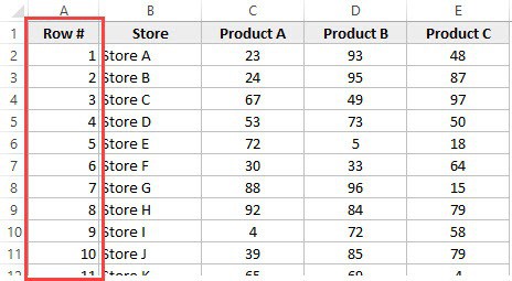
We can number cells in Excel by using the fill handle, or we can automatically number rows by using the ROW function. This article assists all levels of Excel users on how to number cells.
 Figure 1. Final result: How to number cells
Numbering rows
- Select the cell where we want to insert the first row number, say B3, and enter “1”
 Figure 2. Entering the first row number
- Type another value in the next cell to establish a pattern. Enter “2” in cell B4.
 Figure 3. Entering the second row number
- Select cells B3 and B4. The fill handle will appear at the bottom right corner of the selected cells.
 Figure 4. Selecting the first two cells to establish pattern
- Click, hold and drag the fill handle down until the last cell we want to fill.
 Figure 5. Output: Numbering rows
We have now filled the column for row with numbers 1 to 10. However, we have also copied the formatting of cells B3 and B4 and it has distorted the format of our table.
Fill without formatting
In order to fill the row numbers without formatting, we have to drag down the fill handle using the riight-click button of the mouse. When we release the mouse, options will be provided and we can choose Fill without Formatting to achieve the desired result.
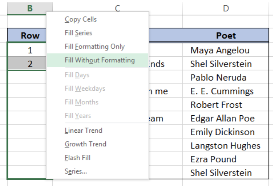 Figure 6. Fill without Formatting option
Finally, we have filled all rows with a row number without distorting the current format of cells.
 Figure 7. Output: Numbering without formatting
Auto numbering
Next, let us learn how to automatically number rows by using the ROW function and an offset value.
- Select the first cell where we want to insert the first row number, say B3
- Enter the sequence formula using the ROW function
= ROW()-2
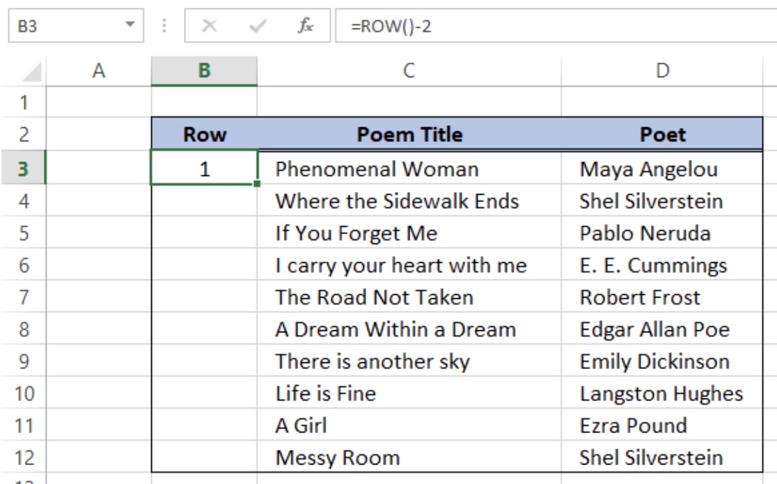 Figure 8. Entering the sequence formula
The ROW function returns the row number of the cell in the worksheet. We have selected cell B3 so the ROW function returns the value 3. Therefore, we need to subtract 2 from the ROW function in order to obtain row number “1” for the first row.
The formula for sequential numbering is therefore given as:
=ROW()-[offset]
In this case, the offset is the number 2.
- Click the fill handle of cell B3 using the right-click button, and drag down to cell B12.
- Choose Fill without Formatting to copy only the formula.
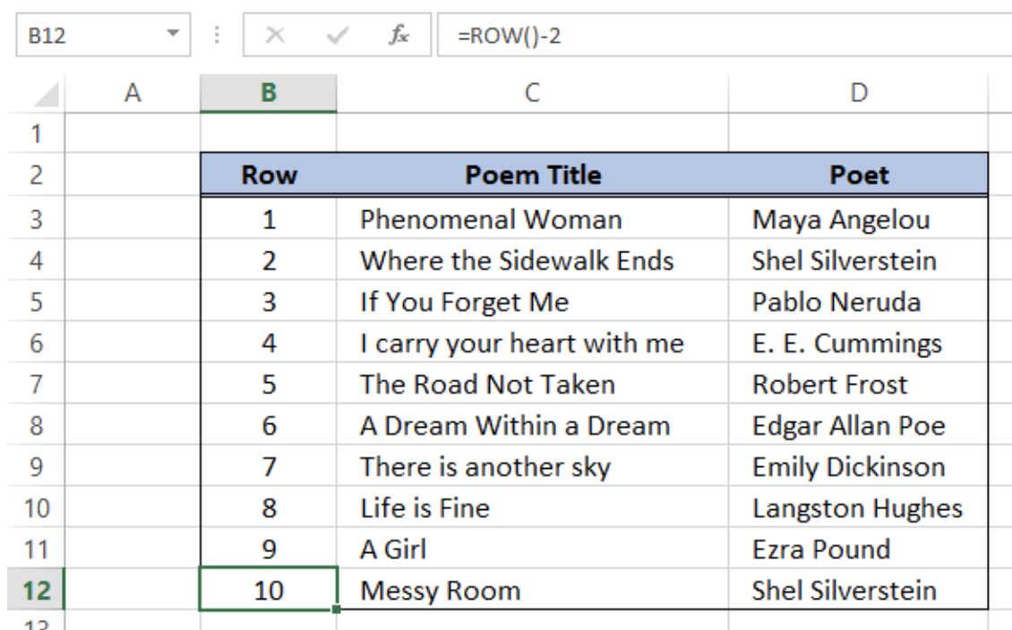 Figure 9. Output: Auto numbering using ROW function
Note that the formula in cell B12 is the same as the formula in cell B3. Finally, we have learned how to number cells by using sequential row numbers.
Instant Connection to an Excel Expert
Most of the time, the problem you will need to solve will be more complex than a simple application of a formula or function. If you want to save hours of research and frustration, try our live Excelchat service! Our Excel Experts are available 24/7 to answer any Excel question you may have. We guarantee a connection within 30 seconds and a customized solution within 20 minutes.
Numbering cells is a task often you’ll often perform in Excel. But writing the number manually in each cell takes a lot of time.
Fortunately, there are methods that help you add numbers automatically. And in this article, I’ll show you two methods of doing so: the first is a simple method, and the second lets you have dynamically numbered cells. So let’s get started.
How to Auto-Number Cells with a Regular Pattern
For this method, you set your starting number in one cell and the next number in the series in the next cell.
Once you have two adjacent cells filled with your two starting numbers, you can select those two cells, click on the handle in the bottom right corner of the green outline, and drag to select all the cells that you want to follow your pattern.
A useful tooltip appears near the bottom right corner of the green outline to show what the last number in the series would be if you released at that point.
So, if you want to start with the number 5 and increment by 3 until 38, you would write 5 in your first cell, and 8 in the next cell. You would then select the cells containing the 5 and the 8, click on the handle, and drag to select the other cells until you see 38 appear in the tooltip. Then you can release, and the numbers will be filled in automatically.
The numbers can also be formatted in descending order: if you start with 7 and then enter 5, the pattern will continue with 3, 1, -1, and so on.
You can also do the same with rows instead of columns. Fill in two consecutive cells in a row with the start of your pattern, then select them and drag the outline horizontally across those cells that you want to continue that pattern. It’ll automatically fill in those numbers.
You can also do the same going upward – fill two cells, select them, click the handle and drag upward to fill the cells above your two starting cells.
Note: this will always add numbers that are evenly spaced in the pattern you’ve started. It won’t work with other kinds of number progressions.
How to Auto-Number Cells Using the ROW() Function
If you have data that can be sorted in different ways (say, a list of names — alphabetically, etc), it’s annoying if the numbering of your lines gets scrambled when you’re sorting other data.
To avoid that, you can dynamically number your rows using the ROW() function.
In the cell where you want the numbering to start, write =ROW(A1). This will produce the number 1 in the cell.
Select the cell and drag the outline from the handle in the corner to populate the same formula in the rest of the cells (or, if you are adding the line numbers near a block of data already present, you can just double-click on the handle on the corner of the selection).
=ROW(A1) in your first cell, 2) It will appear as the number1, 3) Click and drag or double-click to fill all other cells. 4) Now if you sort the data, the line numbers will stay in order.
If you want to have a different regular pattern, you can use a bit of math: to have numbers spaced by 2, you can write =ROW(A1) * 2 in the first cell, and then proceed with the same steps as above. This will produce the numbers 2, 4, 6…and so on.
If you want to change the starting point of the pattern – to maybe have only odd numbers, for example – you can subtract one: =ROW(A1) * 2 - 1, this will produce the numbers 1, 3, 5, 7…
As a general formula, to get any pattern you can write =ROW(A1) * a + b. a is used to determine the step, and b (it can be either a positive or negative number) is used to change the starting point of the pattern.
If you want to number your columns, you can use the COLUMN() function in the same way as the ROW(). Just fill in your first cell with =COLUMN(A1) , select the cell, then expand the selection to the rest of the cells you want your numbers to be in.
Note: if you add or delete rows, you will need to set the auto-numbering again by selecting the first cell and dragging or double-clicking again to restore the pattern.
Conclusion
Writing numbers in cells is a task often performed in Excel, and here we have seen two simple methods that let us save time. The first method just involves writing numbers in two cells, and then a couple of clicks. And the other just requires writing a formula in one cell, and then a couple of clicks.
There are a few other methods for numbering cells in Excel, but these are the most straightforward.
Learn to code for free. freeCodeCamp’s open source curriculum has helped more than 40,000 people get jobs as developers. Get started
Numbering in Excel means providing a cell with numbers like serial numbers to some table. We can also do it manually by filling the first two cells with numbers and dragging them down to the end of the table, which Excel will automatically load the series. Else, we can use the =ROW() formula to insert a row number as the serial number in the data or table.
When working with Excel, some small tasks need to be done repeatedly. However, if we know the right way to do it, they can save a lot of time. For example, generating the numbers in Excel is a task that is often used while working. Serial numbers play a very important role in Excel. It defines a unique identity for each record of your data.
One of the ways is to add the serial numbers manually in Excel. But it can be a pain if you have the data of hundreds or thousands of rows and must enter the row number for them.
This article will cover the different ways to do it.
Table of contents
- Numbering in Excel
- How to Add Serial Number in Excel Automatically?
- #1 – Using Fill Handle
- #2 – Using Fill Series
- #3 – Using the ROW Function
- Things to Remember about Numbering in Excel
- Recommended Articles
How to Add Serial Number in Excel Automatically?
There are many ways to generate the number of rows in Excel.
You can download this Numbering in Excel Template here – Numbering in Excel Template
- Using Fill Handle
- Using Fill Series
- Using ROW Function
#1 – Using Fill Handle
It identifies a pattern from a few already filled cells and then quickly uses that pattern to fill the entire column.
For example, let us take the below dataset.
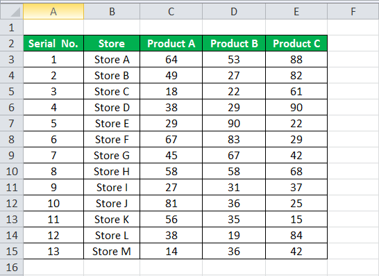
For the above dataset, we have to fill the serial no record-wise. Follow the below steps:
- First, we must enter 1 in cell A3 and insert 2 in cell A4.
- Then, select both the cells as per the below screenshot.

As we can see, a small square is shown in the above screenshot, which is rounded by a red color called “Fill Handle” in Excel.
Place the mouse cursor on this square and double-click on the fill handle.
- It will automatically fill all the cells until the end of the dataset. For example, refer to the below screenshot.

As the fill handle identifies the pattern, fill the individual cells with that pattern.
If you have any blank row in the dataset, the fill handle would only work until the last contiguous non-blank row.

#2 – Using Fill Series
It gives more control over data on how the serial numbers are entered into Excel.
For example, suppose you have below the score of students subject-wise.

Follow the below steps to fill series in the Excel:
- We must first insert 1 in cell A3.
- Then, go to the “HOME” tab. Next, click on the “Fill” option under the “Editing” section, as shown in the below screenshot.

- Click on the “Fill” dropdown. It has many options. Click on “Series,” as shown in the below screenshot.

- It will open a dialog box, as shown below screenshot.

- Click on “Columns” under the “Series in” section. Then, refer to the below screenshot.

- Insert the value under the “Stop value” field. In this case, we have 10 records; enter 10. If we skip this value, the Fill “Series” option may not work.
- Enter “OK.” It will fill rows with serial numbers from 1 to 10. Refer to the below screenshot.

#3 – Using the ROW Function
Excel has a built-in function, which also can be used to number the rows in Excel. To get the Excel row numbering, we must enter the following formula in the first cell shown below:

- The ROW function gives the Excel row number of the current row. We have subtracted 3 from it as we started the data from the 4th. If the data starts from the 2nd row, we must remove 1 from it.
- See the below screenshot. Using =ROW()-3 formula.

Drag this formula for the rest of the rows. The final result is shown below.
Using this formula for numbering will not damage the numbers if we delete a record in the dataset. Furthermore, since the ROW function does not reference cell addresses, it will automatically adjust to give the correct row number.
Things to Remember about Numbering in Excel
- The “Fill Handle” and “Fill Series” options are static. Therefore, if we move or delete any record or row in the dataset, the row number will not change accordingly.
- The ROW function gives the exact numbering if we cut and copy the data in Excel.
Recommended Articles
This article is a guide to Numbering in Excel. We discuss how to automatically add serial numbers in Excel using the fill handle, fill series, and ROW function, along with examples and downloadable templates. You may learn more about Excel functions from the following articles: –
- Auto Numbering in ExcelThere are two approaches for auto numbering. To begin, fill the first two cells with the series you wish to insert and drag it to the table’s end. Second, use the =ROW() formula to get the number, and then drag it to the table’s end.read more
- Row Limit in Excel
- Excel Negative NumberIn Excel, negative numbers, i.e. numbers less than 0 in value, are displayed with minus symbols by default.read more
- IsNumber FunctionISNUMBER function in excel is an information function that checks if the referred cell value is numeric or non-numeric.read more
- Null in ExcelNull is a type of error in Excel that occurs when two or more cell references provided in formulas are wrong, or when their position is incorrect. Using space in formulas between two cell references, for example, will result in a null error.read more
Reader Interactions
Watch Video – 7 Quick and Easy Ways to Number Rows in Excel
When working with Excel, there are some small tasks that need to be done quite often. Knowing the ‘right way’ can save you a great deal of time.
One such simple (yet often needed) task is to number the rows of a dataset in Excel (also called the serial numbers in a dataset).
Now if you’re thinking that one of the ways is to simply enter these serial number manually, well – you’re right!
But that’s not the best way to do it.
Imagine having hundreds or thousands of rows for which you need to enter the row number. It would be tedious – and completely unnecessary.
There are many ways to number rows in Excel, and in this tutorial, I am going to share some of the ways that I recommend and often use.
Of course, there would be more, and I will be waiting – with a coffee – in the comments area to hear from you about it.
How to Number Rows in Excel
The best way to number the rows in Excel would depend on the kind of data set that you have.
For example, you may have a continuous data set that starts from row 1, or a dataset that start from a different row. Or, you might have a dataset that has a few blank rows in it, and you only want to number the rows that are filled.
You can choose any one of the methods that work based on your dataset.
1] Using Fill Handle
Fill handle identifies a pattern from a few filled cells and can easily be used to quickly fill the entire column.
Suppose you have a dataset as shown below:

Here are the steps to quickly number the rows using the fill handle:
Note that Fill Handle automatically identifies the pattern and fill the remaining cells with that pattern. In this case, the pattern was that the numbers were getting incrementing by 1.
In case you have a blank row in the dataset, fill handle would only work till the last contiguous non-blank row.
Also, note that in case you don’t have data in the adjacent column, double-clicking the fill handle would not work. You can, however, place the cursor on the fill handle, hold the right mouse key and drag down. It will fill the cells covered by the cursor dragging.
2] Using Fill Series
While Fill Handle is a quick way to number rows in Excel, Fill Series gives you a lot more control over how the numbers are entered.
Suppose you have a dataset as shown below:
Here are the steps to use Fill Series to number rows in Excel:
This will instantly number the rows from 1 to 26.
Using ‘Fill Series’ can be useful when you’re starting by entering the row numbers. Unlike Fill Handle, it doesn’t require the adjacent columns to be filled already.
Even if you have nothing on the worksheet, Fill Series would still work.
Note: In case you have blank rows in the middle of the dataset, Fill Series would still fill the number for that row.
3] Using the ROW Function
You can also use Excel functions to number the rows in Excel.
In the Fill Handle and Fill Series methods above, the serial number inserted is a static value. This means that if you move the row (or cut and paste it somewhere else in the dataset), the row numbering will not change accordingly.
This shortcoming can be tackled using formulas in Excel.
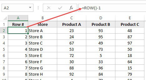
You can use the ROW function to get the row numbering in Excel.
To get the row numbering using the ROW function, enter the following formula in the first cell and copy for all the other cells:
=ROW()-1
The ROW() function gives the row number of the current row. So I have subtracted 1 from it as I started from the second row onwards. If your data starts from the 5th row, you need to use the formula =ROW()-4.
The best part about using the ROW function is that it will not screw up the numberings if you delete a row in your dataset.
Since the ROW function is not referencing any cell, it will automatically (or should I say AutoMagically) adjust to give you the correct row number. Something as shown below:

Note that as soon as I delete a row, the row numbers automatically update.
Again, this would not take into account any blank records in the dataset. In case you have blank rows, it will still show the row number.
You can use the following formula to hide the row number for blank rows, but it would still not adjust the row numbers (such that the next row number is assigned to the next filled row).
IF(ISBLANK(B2),"",ROW()-1)
4] Using the COUNTA Function
If you want to number rows in a way that only the ones that are filled get a serial number, then this method is the way to go.
It uses the COUNTA function that counts the number of cells in a range that are not empty.
Suppose you have a dataset as shown below:
Note that there are blank rows in the above-shown dataset.
Here is the formula that will number the rows without numbering the blank rows.
=IF(ISBLANK(B2),"",COUNTA($B$2:B2))
The IF function checks whether the adjacent cell in column B is empty or not. If it’s empty, it returns a blank, but if it’s not, it returns the count of all the filled cells till that cell.
5] Using SUBTOTAL For Filtered Data
Sometimes, you may have a huge dataset, where you want to filter the data and then copy and paste the filtered data into a separate sheet.
If you use any of the methods shown above so far, you will notice that the row numbers remain the same. This means that when you copy the filtered data, you will have to update the row numbering.
In such cases, the SUBTOTAL function can automatically update the row numbers. Even when you filter the data set, the row numbers will remain intact.
Let me show you exactly how it works with an example.
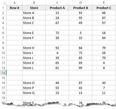
Suppose you have a dataset as shown below:

If I filter this data based on Product A sales, you will get something as shown below:

Note that the serial numbers in Column A are also filtered. So now, you only see the numbers for the rows that are visible.
While this is the expected behavior, in case you want to get a serial row numbering – so that you can simply copy and paste this data somewhere else – you can use the SUBTOTAL function.
Here is the SUBTOTAL function that will make sure that even the filtered data has continuous row numbering.
=SUBTOTAL(3,$B$2:B2)
The 3 in the SUBTOTAL function specifies using the COUNTA function. The second argument is the range on which COUNTA function is applied.
The benefit of the SUBTOTAL function is that it dynamically updates when you filter the data (as shown below):

Note that even when the data is filtered, the row numbering update and remains continuous.
6] Creating an Excel Table
Excel Table is a great tool that you must use when working with tabular data. It makes managing and using data a lot easier.
This is also my favorite method among all the techniques shown in this tutorial.
Let me first show you the right way to number the rows using an Excel Table:
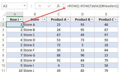
Note that in the formula above, I have used Table2, as that is the name of my Excel table. You can replace Table2 with the name of the table you have.
There are some added benefits of using an Excel Table while numbering rows in Excel:
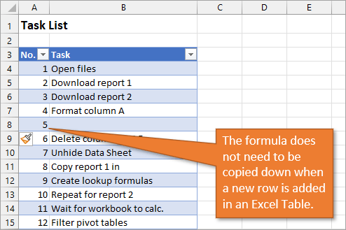
- Since Excel Table automatically inserts the formula in the entire column, it works when you insert a new row in the Table. This means that when you insert/delete rows in an Excel Table, the row numbering would automatically update (as shown below).

- If you add more rows to the data, Excel Table would automatically expand to include this data as a part of the table. And since the formulas automatically update in the calculated columns, it would insert the row number for the newly inserted row (as shown below).


7] Adding 1 to the Previous Row Number
This is a simple method that works.
The idea is to add 1 to the previous row number (the number in the cell above). This will make sure that subsequent rows get a number that is incremented by 1.
Suppose you have a dataset as shown below:
Here are the steps to enter row numbers using this method:
- In the cell in the first row, enter 1 manually. In this case, it’s in cell A2.
- In cell A3, enter the formula, =A2+1
- Copy and paste the formula for all the cells in the column.

The above steps would enter serial numbers in all the cells in the column. In case there are any blank rows, this would still insert the row number for it.
Also note that in case you insert a new row, the row number would not update. In case you delete a row, all the cells below the deleted row would show a reference error.
These are some quick ways you can use to insert serial numbers in tabular data in Excel.
In case you are using any other method, do share it with me in the comments section.
You May Also Like the Following Excel Tutorials:
- Delete Blank Rows in Excel (with and without VBA).
- How to Insert Multiple Rows in Excel (4 Methods).
- How to Split Multiple Lines in a Cell into a Separate Cells / Columns.
- 7 Amazing Things Excel Text to Columns Can Do For You.
- Highlight EVERY Other ROW in Excel.
- How to Compare Two Columns in Excel.
- Insert New Columns in Excel
Bottom Line: Learn 4 different techniques for creating a list of numbers in Excel. These include both static and dynamic lists that change when items are added or deleted from the list.
Skill Level: Beginner
Watch the Tutorial
Download the Excel File
You can download the worksheet that I use in the video here:
If you have a list of items in Excel and you’d like to insert a column that numbers the items, there are several ways to accomplish this. Let’s look at four of those ways.
1. Create a Static List Using Auto-Fill
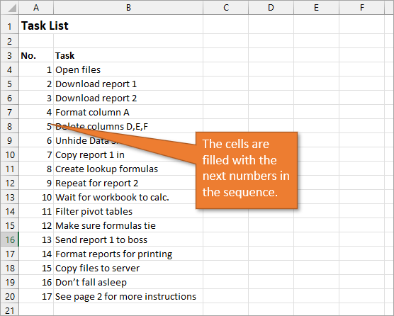
The first way to number a list is really easy. Start by filling in the first two numbers of your list, select those two numbers, and then hover over the bottom right corner of your selection until your cursor turns into a plus symbol. This is the fill handle.
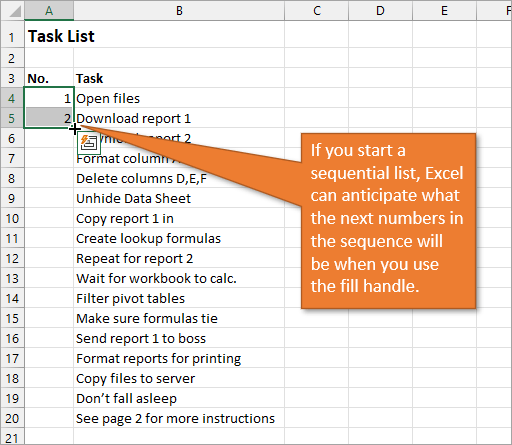
When you double-click on that fill handle (or drag it down to the end of your list), Excel will fill in the blanks with the next numbers in the sequence.
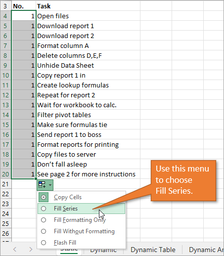
An alternate way to create this same numbered list is to type a 1 in the first cell and then double-click the fill handle. Because Excel doesn’t have a second number to identify a sequence or pattern, it will fill down the columns with 1s. But you will notice that a menu is available at the end of your column, and from that menu, you can select the option to Fill Series. This will change the 1s to a sequential list of numbers.
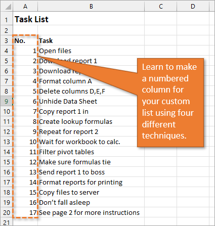
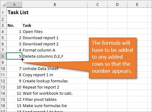
The numbered column we’ve created in both instances is static. This means it doesn’t change when you make additions or deletions to the corresponding list of items. For example, if I insert a new row in order to add another task, there is a break in the numbered column as well, and I would have to repeat the same steps to correct the list.
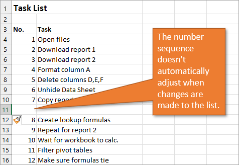
So, unless we want the numbers to always remain as they are, a better option would be to create a dynamic list.
2. Create a Dynamic List Using a Formula
We can use formulas to create a dynamic list where the numbers update when we add or delete rows from the list.
To use a formula for creating a dynamic number list, we can use the ROW function. The ROW function returns the row number of a cell. If we don’t specify a cell for ROW, it just returns the current row number of whatever is selected.
In our example, the first cell in our list doesn’t start on Row 1. It starts on Row 4. But we don’t want our list to start at 4; we want it to start at 1. To subtract the extra 3, our formula will include a minus sign and then the ROW function again, but this time pointed to the cell above our formula (which is in Row 3).
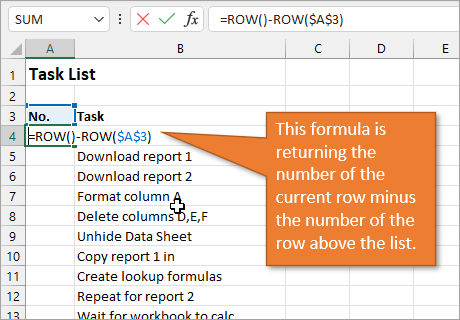
We use the absolute values (dollar signs) in our cell selection because we don’t want that number to change as we copy the formula down the list. In other words, we always want to subtract 3 from the row number to give us our list number.
When we copy down the formula, we have a numbered list that will adjust when we add or delete rows. However, when adding a row, we will have to copy the formula into the newly inserted cell.
This additional step of copying the formula into new rows can be avoided if we use Excel Tables.
3. Create a Dynamic List Using a Formula in an Excel Table
If we write the same formula but we use an Excel table, the only difference we will make in the formula is that we reference the column header instead of the absolute cell value.
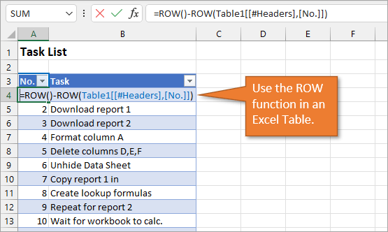
Because we are using an Excel Table, the formula automatically fills down to the other rows. When we add a row to the table, the formula will automatically populate in the new cell.
4. Create a Dynamic List Using Dynamic Array Formulas
Below, I have a table that is populated using Dynamic Array Formulas. The FILTER formula spills a range of results based on whatever name is selected in the orange cell.
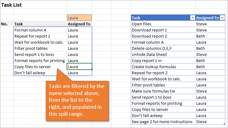
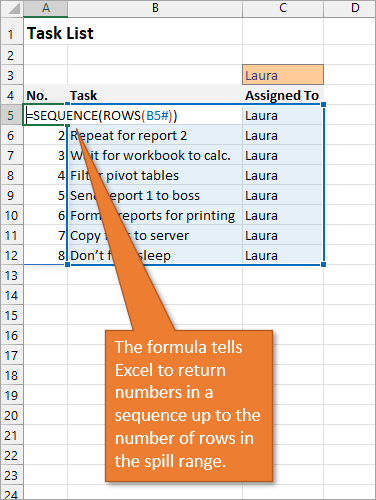
The Dynamic Array formula we will use is SEQUENCE. This will return a sequence for the number of rows we identify in the formula. To tell Excel how many rows there are, we will use the ROW function as the argument for sequence. The argument for ROW is just the spill range. The way to notate the spill range is to simply place a hashtag after the name of the first cell in the range. So our formula looks like this:
=SEQUENCE(ROWS(B5#))
Once we complete our formula and hit Enter, the list will be numbered.
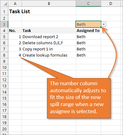
With this formula in place, if the size of the range changes when a new name is selected, the numbered column for the list will automatically adjust as well.
Bonus Tip: Formatting Your Numbered List
If you want to add periods or other punctuation to your numbered list:
- Select the entire list and right-click to choose Format Cells. Or use the keyboard shortcut Ctrl + 1.
- Choose the Custom option on the Number tab.
- Then in the Type field, type in the number 0 with whatever punctuation you would like to surround your number.
Here, I’ve just added a period.
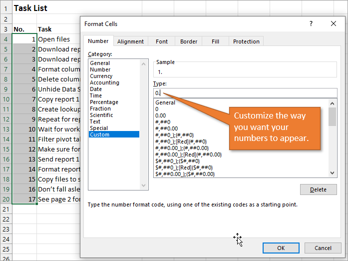
When you hit OK, you will have formatted the entire selection.
Related Posts
Here are a few similar posts that may interest you.
- Excel Tables Tutorial Video – Beginners Guide for Windows & Mac
- New Excel Features: Dynamic Array Formulas & Spill Ranges
- How to Prevent Excel from Freezing or Taking A Long Time when Deleting Rows
Conclusion
I hope these four ways to create ordered lists are helpful for you. If you have questions or feedback, I would love to hear them in the comments. Have a great week!